


ABSTRACT
Spectroscopic observations of  Cyg (K0 III) taken over 12 seasons from 1999 to 2010 with a resolving power ∼100,000 are analyzed for radial velocities, granulation properties, and projected rotation rate. The new radial velocities, which are on an absolute velocity scale with convective blueshifts removed, contribute to the determination of the 55-year orbit parameters, but are insufficient to be definitive. Line-depth ratios show photospheric temperature variations amounting to ∼4 K, likely arising from a magnetic cycle. A small velocity variation, ∼100 m s−1, may mimic the temperature variations. Fourier analysis of the line broadening yields the projected rotation rate v sin i = 1.0 ± 0.2 and macroturbulence dispersion
  = 4.45 ± 0.05 km s−1. A possible rotation modulation in velocity with a period of ∼1.5 years is noted. The third signature of granulation, i.e., greater blueshifts for weaker lines, is measured and indicates a photospheric velocity gradient in Cyg that is 1.1 ± 0.1 times the Sun's, which is consistent with previously measured K giants. Mapping the line bisector of the Fe i λ6253 line on to the third-signature plot results in a flux deficit with a maximum 4.9 km s−1 redward of the line core and an amplitude of 16.5% ± 0.5% of the core depth, values typical of K giants. A 145 K disk-averaged temperature difference between granules and lanes is implied.
Export citation and abstract BibTeX RIS
1. INTRODUCTION
Analysis of the spectra of cool stars like Cyg (K0 III, HR 7949, HD 197989, HIP 102488) is challenging because the Doppler shifts of the star's rotation, granulation, microturbulence, and thermal motions are of comparable size. But rotation and granulation are the cornerstones of the dynamics of cool-star atmospheres and therefore of considerable importance. The projected rotation velocity and granulation characteristics of Cyg are extracted in the analysis below. Since a 12 year time span is covered by the observations, variations in temperature and velocity are also established, and a contribution is made to the star's orbital data.
Using the apparent magnitude of 2.48 ± 0.009 and parallax of 44.86 ± 0.12 mas from the SIMBAD database, the absolute magnitude is 0.74 ± 0.02. This places the star squarely in the class III domain of the HR diagram, although a classification of III–IV is occasionally assigned (Gray et al. 2003). For the modeling done below in Section 5, values of effective temperature, surface gravity, and metallicity are needed, although the results of the modeling are only weakly dependent on the adopted values. Published effective temperatures generally range between 4700 and 4800 K (e.g., McWilliam 1990; Luck & Challener 1995; Gray et al. 2003; Massarotti et al. 2008; Prugniel et al. 2011). I adopted 4750 K. From these same references, log g ranges from 2.4 to 2.9. I adopted 2.5. The angular diameter given by Mozurkewich et al. (1991) is 4.62 ± 0.04 mas, or a radius of 11.1  . A mass ∼2 solar masses, which is reasonable for a K0 giant, is consistent with the adopted surface gravity. Metallicity, again from these same references, ranges from −0.27 to −0.10. I adopted −0.20.
This giant is a single-spectrum binary with a five-decade period and a very eccentric orbit (Griffin 1994). Radial-velocity observations between 2000 and 2010, as presented below, place some additional constraint on the orbital solution. The new results basically support Griffin's analysis but with slightly different orbital parameters. Possible characteristics of the unseen secondary star are discussed in some detail by Griffin (1994). Velocity variations on shorter timescales are ≲100 m s−1 (see below) and may arise from convection, non-radial oscillations, or surface features and rotational modulation. Such variations are common in evolved stars (e.g., Walker et al. 1989; Hatzes & Cochran 1993; Gray & Brown 2006; Kiss et al. 2006; Carney et al. 2008; Eaton et al. 2008; Gray 2008, 2010b, 2013; Stothers 2010; Hekker et al. 2011; Huber et al. 2011; Gray & Pugh 2012).
There are rather few published values of the projected rotation rate of Cyg. The results of previous Fourier analyses, Gray & Martin (1979), 2.1 ± 0.5 km s−1, and Gray (1982), 3.0 ± 0.6 km s−1, are now replaced by the significantly smaller value found in the analysis below. Other determinations are based on calibrated half widths or calibrated cross-correlation techniques, often with assumed values of macroturbulence broadening: Fekel (1997), 2.0 ± 0.7 km s−1, De Medeiros & Mayor (1999), 1.4 ± 1.0 km s−1, Hekker & Meléndez (2007), 3.01, and Massarotti et al. (2008), 1.4 ± 1.2 km s−1.
This is the second paper of a planned series in which detailed line-profile analysis is done for stars using high resolution, high signal-to-noise data. The analysis of β Gem (Gray 2014) is in Paper 1.
2. THE OBSERVATIONS
The coudé spectrograph at the Elginfield Observatory (Gray 1986, 2005b) was used to acquire 68 exposures in the ninth grating order during the 1999–2010 observing seasons. Fifteen of these were taken in the first two years, prior to installation of the radial-velocity capability (Gray & Brown 2006), but they are still useful for line-broadening and line-depth-ratio work. The nominal signal-to-noise ratio (S/N), based on the CCD signal levels, range from 260 to 590 with a mean of 395 (median 388). The resolving power is λ/Δλ ∼ 100,000. This is an important asset of these data because for values as low as ∼50,000 (typical of many so-called high-resolution spectrographs) the line bisector shapes are severely compromised. Similarly, the ability to extract from the line shapes the small rotation rates of cool giants like Cyg is critically dependent on the resolving power. Other information about the spectrograph and reduction procedures can be found in Paper 1.
As can be seen in Figure 1, which shows the full recorded wavelength range, most of the lines are blended to greater or lesser degree. There are only a few short spans where the continuum is passably undistorted by weak lines and they were used to normalized the continuum to unity. 45 of the lines were used for radial-velocity work, 32 have absolute wavelengths and were used for the third-signature plots, and only 13 were sufficiently unblended to be useful for the rotation/macroturbulence analysis.
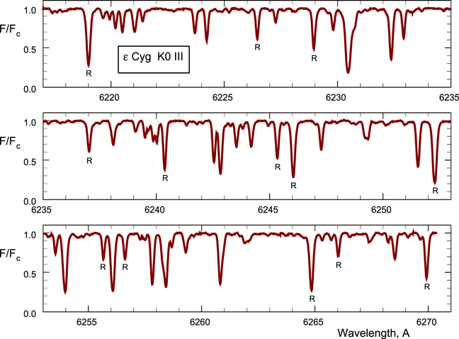
Figure 1. Ordinate is flux normalized by the continuum value. This wavelength region has relatively modest blending but it remains a serious problem. Very few lines have even one unblended wing and the plethora of weak lines makes setting the continuum a challenge. Lines used in the rotation/macroturbulence analysis are tagged with an R.
Download figure:
Standard image High-resolution image3. RADIAL VELOCITIES
Forty-five lines in 53 exposures of Cyg were measured for radial velocity. The core velocities and depths were measured by fitting a parabola to the core points of the line profiles. The absolute wavelengths of the stellar lines are tied to the laboratory measurements of Fe i done by Nave et al. (1994), which give the rest wavelengths. Additional lines from a previous work were added (Gray & Pugh 2012). The observed stellar line positions were established using water vapor lines with known wavelengths (Chevillard et al. 1989) formed inside the coudé spectrograph. The technique has similarities to absorption-cell and telluric-line methods, but also has important differences. Details can be found in Gray & Brown (2006).
Mean velocities for each exposure were computed using weighting inversely proportional to the scatter shown by each line across the 53 exposures. Lines toward the edges of the field show larger scatter because the water-vapor lines do not fix the dispersion as precisely as near the center of the field. The mean absolute velocities are listed in Table 1. These values are corrected for the convective blueshifts established from the third-signature plot (Section 6). The errors are computed from the standard deviations around the season means and the relative weights of the exposures based on the scatter in the third-signature plots. The average error is ∼85 m s−1, but some seasons have very few measurements, so this is an approximate number. However, since short term variations are included, the actual measurement error is expected to be slightly smaller.
Table 1. Absolute Radial Velocities (m s−1)
| Year | JD-2450000 | Velocity | Err |
|---|---|---|---|
| 2001.5406 | 2105.826 | −12948 | ±89 |
| 2001.6171 | 2133.729 | −13121 | ±78 |
| 2001.6416 | 2142.691 | −12863 | ±133 |
| 2001.6880 | 2159.618 | −12925 | ±118 |
| 2001.7071 | 2166.574 | −12856 | ±91 |
| 2002.4749 | 2446.852 | −12716 | ±133 |
| 2002.5159 | 2461.812 | −12767 | ±111 |
| 2002.5462 | 2472.863 | −12740 | ±59 |
| 2002.5488 | 2473.816 | −12777 | ±43 |
| 2002.5542 | 2475.771 | −12822 | ±90 |
| 2002.5679 | 2480.772 | −12775 | ±94 |
| 2002.6092 | 2495.873 | −12849 | ±70 |
| 2002.7180 | 2535.576 | −13057 | ±88 |
| 2002.7291 | 2539.609 | −12810 | ±168 |
| 2003.4832 | 2814.865 | −12846 | ±185 |
| 2003.5380 | 2834.868 | −12834 | ±54 |
| 2003.5461 | 2837.827 | −12956 | ±54 |
| 2003.5515 | 2839.792 | −12813 | ±81 |
| 2003.7866 | 2925.622 | −12938 | ±74 |
| 2004.4518 | 3168.857 | −12792 | ±61 |
| 2004.5882 | 3218.777 | −12910 | ±59 |
| 2004.6481 | 3240.712 | −12969 | ±232 |
| 2004.6700 | 3248.704 | −12916 | ±41 |
| 2004.7024 | 3260.592 | −12930 | ±85 |
| 2004.7462 | 3276.622 | −13167 | ±23 |
| 2004.7816 | 3289.552 | −12923 | ±85 |
| 2004.8225 | 3304.530 | −12928 | ±181 |
| 2004.8469 | 3313.472 | −12880 | ±67 |
| 2005.4831 | 3545.847 | −13080 | ±126 |
| 2005.5625 | 3574.813 | −13057 | ±28 |
| 2005.6525 | 3607.671 | −13052 | ±45 |
| 2005.7182 | 3631.658 | −13049 | ±76 |
| 2005.7456 | 3641.657 | −13171 | ±16 |
| 2005.8493 | 3679.497 | −13123 | ±62 |
| 2006.4612 | 3902.841 | −13043 | ±67 |
| 2006.8329 | 4038.519 | −13147 | ±104 |
| 2006.8385 | 4040.536 | −13091 | ±101 |
| 2006.9014 | 4063.496 | −12932 | ±69 |
| 2007.5707 | 4307.798 | −13198 | ±183 |
| 2007.5898 | 4314.784 | −13172 | ±124 |
| 2007.6745 | 4345.700 | −13276 | ±95 |
| 2007.7155 | 4360.663 | −13357 | ±101 |
| 2007.8225 | 4399.708 | −13033 | ±103 |
| 2008.5447 | 4663.873 | −13262 | ±42 |
| 2008.6970 | 4719.611 | −13294 | ±50 |
| 2008.7218 | 4728.689 | −13182 | ±129 |
| 2008.8119 | 4761.647 | −13164 | ±86 |
| 2008.8172 | 4763.584 | −13066 | ±143 |
| 2009.5353 | 5025.874 | −13311 | ±30 |
| 2009.7128 | 5090.669 | −13374 | ±58 |
| 2010.5133 | 5382.872 | −13496 | ±51 |
| 2010.6581 | 5435.691 | −13705 | ±104 |
| 2010.7864 | 5482.534 | −13571 | ±164 |
Download table as: ASCIITypeset image
For well over a century, radial velocities have been measured for Cyg, starting with the 1896 Lick observations of Campbell & Moore (1906). Griffin (1994) discussed and analyzed the available values, including many of his own, through early 1993. These comprise a rather heterogeneous mix of instruments, observers, and reduction techniques. In addition to the modest precision associated with early observations, estimated by Griffin to be in the 1–2 km s−1 range, there is the complication of different zero points for different data sets. Even after zero-point adjustments, there are deviations somewhat larger than might be expected, as can be seen in Figures 2 and 3 of Griffin (1994) and included here in slightly modified form in Figure 2. Nevertheless, and this is the important point made by Griffin, the data are sufficient to show a sharp change in 1906 indicative of orbital motion for a binary with a highly eccentric orbit. Unfortunately the 1961 periastron passage was not observed. The data assembled by Griffin allow only an approximate orbit determination.
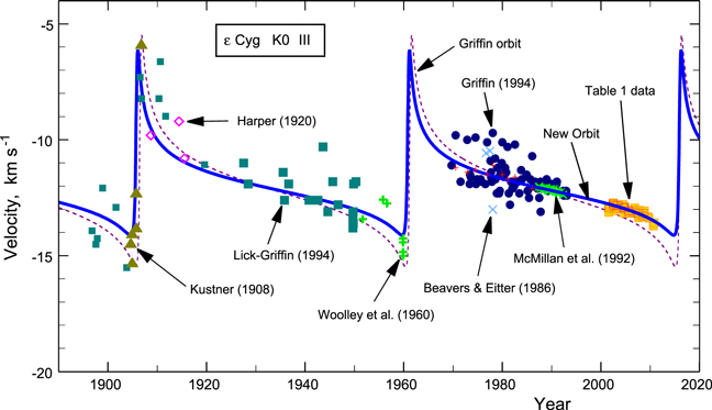
Figure 2. Composite of radial velocities from Griffin (1994), McMillan et al. (1992), and the new Elginfield values in Table 1. The orbit chosen by Griffin (with slightly revised gamma velocity) and the new orbit are both shown as lines. Thirteen spurious Lick values between 1927 and 1934, as identified by Griffin, have been omitted. The nine Griffin values standing above the others (1970–1986), brought down by 1.3 km s−1, are shown as small crosses.
Download figure:
Standard image High-resolution imageA new orbit is shown here in Figure 2 and is listed with Griffin's parameters in Table 2. For convenience, all three times of periastron passage are given. The systemic or gamma velocity is −12.01 (convective blueshifts have been removed, but not gravitational redshift). This orbit was derived as follows. The Elginfield data serve as an anchor or starting point since they are on an absolute, blueshift corrected, scale (see Section 6 below). Orbital parameters were adjusted until systematic differences across the nine years of observation were minimized. The orbital eccentricity has the greatest leverage on the slope of the radial-velocity curve in the 2001–2010 decade, with lesser changes arising from variations in the longitude of periastron, the velocity amplitude, and the epoch of periastron passage. The crosstalk among these variables means that a definitive orbital solution is not yet possible. The second step was to incorporate the McMillan et al. (1992) data, which are completely relative, to place them on the orbital curve. Although the McMillan et al. data are relative, they have such high precision that their slope over the ∼ five years of observation give a significant constraint on the orbit, especially its eccentricity. In a similar manner, the measurements by Griffin (1994), were systematically lowered by 0.1 km s−1 to agree with the Elginfield zero point. Griffin (1994) discusses relative zero points for the other data he assembled and I have made additional minor adjustments on these. As already noted by Griffin, ∼ a dozen Lick values around 1927–34 appear to be ∼2 km s−1 too high owing, he speculated, to a spurious reference spectrum and measurement technique. These discordant values have been omitted from Figure 2. I note in passing that the 1969–93 data of Griffin (solid dots) show a series of nine points lying systematically above the rest. If these are brought down by 1.3 km s−1, they fit the orbit rather well. Finally it should be noted that the next periastron swing, which lasts approximately two years and can give definitive orbit parameters, is currently in progress with zero-velocity crossing predicted to be in late 2015 September and periastron passage near 2016.0.
Table 2. Preliminary Orbital Parameters
| Parameter | Griffin | Gray |
|---|---|---|
| P (years) | 54.76 | 55.1 |
| T0(date) | 1906.52 | 1905.80 |
| 1961.28 | 1960.90 | |
| 2016.04 | 2016.00 | |
| ω (degrees) | 290 | 300 |
| e | 0.9 | 0.9 |
| K (km s−1) | 5.0 | 4.0 |
Download table as: ASCIITypeset image
Much shorter timescale variations were pointed out by McMillan et al. (1992). Variations around the orbital motion are taken to be intrinsic to the star. Stellar velocity variations have been seen in other binaries (e.g., Eaton et al. 2008; Gray 2012; Pugh & Gray 2013), but are also common in single stars. For evolved stars, non-radial oscillations produce variations on shorter timescales of hours and days, while convection, rotational modulation, and magnetic cycles cause variations on longer timescales of months, years, and decades respectively. The residual velocities of Cyg are discussed below.
4. LINE-DEPTH RATIOS—TEMPERATURE VARIATIONS
The ratio of core depths of temperature-sensitive lines to temperature-stable lines has now become a routine way to measure small temperature changes (e.g., Gray & Brown 2001; Catalano et al. 2002; Kovtyukh et al. 2006; Gray 2008; Kim et al. 2012; Ramm 2015). Eleven ratios were used for Cyg, ten of which are listed in Table 1 of Paper 1. Observational errors in line-depth ratios can be assessed from the standard deviations over the 68 exposures, assuming no intrinsic stellar variation. The circles in Figure 3 show the standard deviations normalized to line-depth ratio as a function of the line depth of the numerator line. An approximate estimate of the expected errors can be made by combining the errors of the individual line depths, namely, ![${[{({e}_{1}/{d}_{1})}^{2}+{({e}_{2}/{d}_{2})}^{2}]}^{1/2}$](https://content.cld.iop.org/journals/0004-637X/810/2/117/revision1/apj518867ieqn3.gif) , where e1 and e2 are the errors on depths d1 and d2. If we then take e1 = e2 = 1/300, the reciprocal of an effective S/N, we find the crosses in Figure 3. The general trend is reproduced, which confirms the noise dependence on line depths. As stated in Section 2, the mean S/N in the continuum is 395. The main reason the effective S/N is reduced to ∼300 is the smaller photon count in the line cores. In fact, the average core depth of the 22 lines used is ∼0.4 for a flux reduction to 0.6 of the continuum value. Then the expected S/N is reduced to 395 ×
, where e1 and e2 are the errors on depths d1 and d2. If we then take e1 = e2 = 1/300, the reciprocal of an effective S/N, we find the crosses in Figure 3. The general trend is reproduced, which confirms the noise dependence on line depths. As stated in Section 2, the mean S/N in the continuum is 395. The main reason the effective S/N is reduced to ∼300 is the smaller photon count in the line cores. In fact, the average core depth of the 22 lines used is ∼0.4 for a flux reduction to 0.6 of the continuum value. Then the expected S/N is reduced to 395 ×  = 306 ∼ the effective S/N.
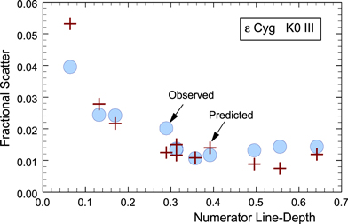
Figure 3. Comparison of observed to predicted scatter in line-depth ratios.
Download figure:
Standard image High-resolution imageEach line-depth ratio has its own temperature sensitivity. The sensitivity factors were found empirically by plotting line-depth ratios for several giant stars against the effective temperatures of those stars. The individual line-depth ratios were converted to temperature variations by subtracting off the mean and multiplying by the sensitivity factor. When all 11 ratios were processed in this way, they were averaged using weights inversely proportional to the scatter shown by each ratio. The season means are shown as a function of time in Figure 4. The average season error is 1.4 K. Over the limited time period of the observations, the temperature rises and falls with an amplitude ∼3–4 K.
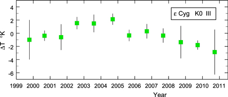
Figure 4. Season means of line-depth-ratio temperature variations based on 11 ratios. Error bars indicate the standard deviation within each season.
Download figure:
Standard image High-resolution imageBased on model photosphere computations, a 4 K variation in effective temperature would be expected to produce a 4 mmag variation in visual flux. HIPPARCOS photometry of Cyg, as shown in Figure 5, were averaged in two-month bins so as to smooth out any variations arising from non-radial oscillations. The amplitude of the photometric variations is quite compatible with the spectroscopic temperature variations, although the timescale may differ. Of course, the HIPPARCOS and Elginfield data do not cover the same time period.
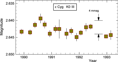
Figure 5. HIPPARCOS visual magnitude data averaged in two-month bins. Error bars indicate the standard deviation within each bin.
Download figure:
Standard image High-resolution imageVariations on such decade timescales are likely associated with magnetic cycles (e.g., Wilson 1978; Baliunas et al. 1998; Gray & Baliunas 1997; Gray & Livingston 1997; Hall et al. 2007). Although detailed documentation of magnetic cycles in giants is sparse, there seems to be a wide variety of HK-emission behavior. For example, among the four Hyades K0 giants, between 1984 and 1995, δ Tau shows ∼7 year cycle, Tau shows a smooth, low-amplitude minimum, γ Tau shows greater activity of an irregular nature, and  Tau shows even more activity with possibly a ∼15 year cycle (Baliunas et al. 1998). Similarly, three K0 giants in the Praesepe cluster show low-level, slowly varying HK, while a fourth shows stronger and irregular HK behavior. So even among stars of similar age and evolutionary status no one pattern is seen. Within this context, the variation Cyg is not out of step and a cycle with something like a 20 year period may be in play.
There may be a correlation between the velocity and temperature variations. The two variables are compared in Figure 6. The vertical scaling between the two plots is arbitrary. For nine of the 10 seasons, the agreement is within the errors. The one apparent discrepancy is in 2009, where there are only three observations, making the internal error itself rather uncertain. In fact, if the average temperature error per exposure is used, reduced by the square root of the three observations, the error in 2009 would be more comparable to those of 2008 and 2010.
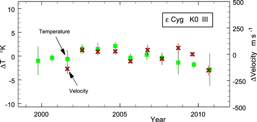
Figure 6. Season-mean velocity variations are compared to season-mean temperature variations.
Download figure:
Standard image High-resolution imageThe physical cause of the ∼3–4 K temperature and the ∼100 m s−1 velocity variation remains to be identified. A small global change in the photospheric temperature alone would not account for the velocity variation (if it is real). Possibly some change in photospheric structure might alter the line-depth ratios. One constraint can be put in place by comparing the temperature variations of individual line-depth ratios to their mean as a function of line strength, where line strength is a proxy for depth of formation. The conclusion is: the line-depth ratio results do not depend on depth of formation; no systematic differences are seen for line depths ranging from 0.29 to 0.75. Other possibilities exist such as a variation in the fraction of the surface permeated by magnetic fields. More magnetic area or stronger fields implies a more transparent photosphere owing to the displacement of gas pressure by magnetic pressure. This in turn would raise the average apparent surface temperature, but would also shift the average convective velocity toward that of deeper layers, i.e., a stronger blueshift, opposite what is seen in Figure 6, unless the convective velocities are inhibited in the magnetic regions. Finally, starspots might be expected to vary during a magnetic cycle, at least judging from the solar case. Changes in the solar irradiance over the solar cycle is also well documented (Solanki et al. 2013). Starspots, through rotational modulation, might induce small velocity variations. Considerable work remains to be done here. No such variations were seen in β Gem (Paper 1).
5. ANALYSIS OF LINE BROADENING FOR ROTATION AND MACROTURBULENCE
The analysis here follows the pattern detailed in Paper 1. Thirteen lines in the recorded spectral interval were sufficiently unblended to be useful (tagged with Rs in Figure 1). In virtually all cases, some correction for line blending was necessary. Corrections for λ6253 are the smallest; for λ6229 the largest. Often one wing is "damaged" and the opposite wing was reflected back around line center to enable a reconstruction. After correcting for blends, the Fourier transform was computed. These are the lowest set of plots shown in Figure 7.
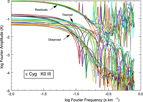
Figure 7. Transforms of all lines used in the rotation-macroturbulence analysis are shown. There is good agreement among the residual transforms. The residual transforms can only be followed up to log frequency ∼−0.75, beyond which amplified noise dominates.
Download figure:
Standard image High-resolution imageUnder the usual assumption that the thermal profile is convolved with the Doppler-shift distribution from rotation and macroturbulence, the transforms of the thermal profiles (middle set of plots in Figure 7) were divided into the transforms of the observed lines to obtain the residual transforms (topmost set of plots in Figure 7). Thermal profiles were computed from an LTE model photosphere using an effective temperature of 4750 K, a log g of 2.5, and [Fe/H] = −0.20, as adopted in Section 1 above. A temperature distribution based on Ruland et al. (1980), as explained in Paper 1, was used. A value of microturbulence dispersion, ξ, was chosen independently for each line. Four lines are sufficiently strong to show sidelobes in their transforms and allow a clear value of microturbulence dispersion to be measured. They are: λ6219, ξ = 1.84; λ6246, ξ = 1.01; λ6253, ξ = 1.55; and λ6265, ξ = 0.99 km s−1. For the weaker lines, where ξ has relatively little affect, values near 1.0 km s−1 were used.
If the broadening from rotation and macroturbulence is the same for all lines, we expect all residual transforms to be the same. Indeed, the scatter of the residual transforms is a measure of the veracity of this statement as well as being a measure of the precision of the analysis. There is quite reasonable agreement among the residual transforms and the scatter is no more than expected from the uncertainty in the blend corrections. To reiterate a point or two made in Paper 1, transforms of the observed profiles plunge below the noise level near an ordinate ∼−4. Division by the transforms of the thermal profiles results in amplified noise for abscissa values above ∼0.75, with individual noise spikes at lower frequencies corresponding to the first zero positions of the four strong lines. The strongly amplified noise is basically ignored in the rest of the analysis. The mean residual transform is computed along with the scatter and standard error. Although it makes only a small difference, the four strong lines are omitted from the mean because (1) the amplified noise around their first zero positions reduces our ability to follow the transform to high frequencies and (2) the strong lines are more dependent on any uncertainty in the temperature distribution, while the weak lines are much less so. The mean residual for the remaining nine lines and its errors are shown in Figure 8. The error bars are smaller than the symbols for low frequencies and grow very large for the high frequencies dominated by amplified noise.
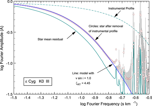
Figure 8. Mean residual transform from Figure 7 is shown by the lowest line. The model (line) with v sin i = 1.0 and  = 4.45 is compared to the mean residual transform (circles) after removal of the instrumental profile. Amplified noise is seen on the right. Error bars represent the standard deviation of the mean residual transform. They are smaller than the symbols for abscissas to the left of ∼−0.75.
Download figure:
Standard image High-resolution imageThe instrumental profile was measured numerous times during the span of the observations using λ5461 from an isotopic mercury bulb excited by microwaves and cooled with a continuous air flow. The uppermost curve in Figure 8 is the transform of the instrumental profile that was divided into the mean residual transform to give the final result, the transform of the combined Doppler-shift distribution of rotation and macroturbulence, that is to be modeled.
As explained in several previous publications, e.g., Paper 1, disk integrations are used to combine the Doppler shifts of radial-tangential macroturbulence and rotation. Limb darkening for the disk integrations was computed explicitly for the assumed temperature distribution. The macroturbulence dispersion is denoted by  . The values of v sin i and
  were adjusted until the model transform agreed with the observations. The result is shown in Figure 8 and the final values are

The errors are estimated by computing models that correspond to the upper and lower error bars on the transform. As can be seen in Figure 8, the final model is not a perfect fit, but is within the observational errors.
This value of v sin i is smaller than most previous determinations (Section 1), while  is not only similar to the 4.53 ± 0.10 km s−1 found for β Gem in Paper 1, but agrees very well with the trend for class III giants shown in Figure 8 of Gray & Pugh (2012).
The Fourier solution was then used to model the profiles directly and four examples are given in Figure 9. The agreement is very good.
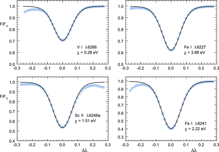
Figure 9. Examples of model profiles (lines) compared to the observations (symbols). The model profiles have v sin i = 1.0 and  = 4.45 that were determined from the Fourier solution shown in Figure 8. Note the slightly different ordinate scales among the four plots.
Download figure:
Standard image High-resolution imageBefore moving on, let us reconsider the fairly common practice of using a Gaussian distribution for the macro-blurring instead of disk integrations. Conceptually this amounts to neglecting rotational broadening and assuming an isotropic Gaussian velocity distribution for the macroturbulence, even though we know rotational broadening does exist and macroturbulence is not isotropic. In other cases, a quadratic combination of v sin i and  is assumed even though this process is only appropriate for isotropic Gaussians (e.g., Benz & Mayor 1984; Melo et al. 2001; Allende Prieto et al. 2004; Hekker & Meléndez 2007; Massarotti et al. 2008; Takeda et al. 2008). The fact that when
  is comparable to v sin i, the resultant disk integration is close to Gaussian (e.g., Gray 1978, 2005b, p. 481) is a temptation, and rather passable fits to observed profiles can be obtained with Gaussian blurring. For Cyg, where v sin i is considerably smaller than
  , one has to look closely at the profiles to see the mismatch. Figures 10 illustrates this and Figure 11 shows how the mismatch in the Fourier domain is not so easily missed. The more clear separation in the Fourier domain is partly because of the difference in the way shape information is displayed in the two domains, but also because the Fourier plot shows only the rotation/macroturbulence portion of the broadening, while the line profiles include the thermal/microturbulence component as well.
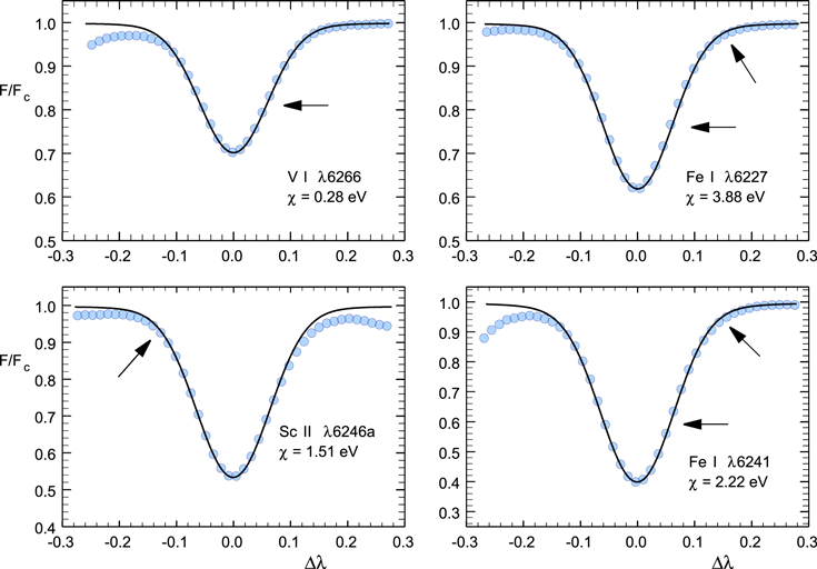
Figure 10. Inadequate modeling using Gaussian macro-broadening. Circle are observations, lines are the models. Small but significant systematic mismatches can be seen, especially in the wings (angled arrows), where the model wings are too weak, and in the basic line widths (horizontal arrows), where the models are systematically too wide. A Gaussian dispersion of 3.28 km s−1 was used.
Download figure:
Standard image High-resolution image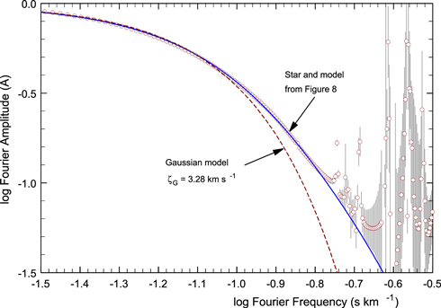
Figure 11. Transform of the same Gaussian used in Figure 10 is shown in the Fourier domain along with the adopted solution and observations from Figure 8.
Download figure:
Standard image High-resolution imageConsequently, if the object is to model an observed spectrum for abundance analysis, for example, then Gaussian blurring might be acceptable. But one would be amiss to go on to interpret the Gaussian's width as macroturbulence. Also, as pointed out some time ago (Gray 1978), the isotropic Gaussian  is ∼30% smaller than the radial-tangential
  giving the same broadening.
A radius of 11.1 solar radii with v sin i = 1.0 km s−1 implies a rotation period of 1.55 years or less by sin i. Although the radial-velocity data of McMillan et al. (1992) covers only a relatively short time span, a periodogram of these data has a weak peak at ∼0.658 cycle  , or a period of 1.52 years. Figure 12 shows the McMillan et al. data (with the orbital component removed) compared to a sinusoid with this period. Naturally one should bear in mind that if surface features are the cause of modulation, any intrinsic variation in the features could result in velocity amplitude and phase changes from one cycle to the next. Although hardly conclusive, the figure is suggestive. Unfortunately the errors in the Elginfield velocities are too large to contribute to the issue. Also to be noted is that for the Sun, McMillan et al. (1993) saw no velocity variations exceeding 8 m s−1 over a 4.9-year span, a substantial portion of a solar cycle. As noted at the end of Section 3 above, non-radial oscillations are expected to occur on considerably shorter timescales (e.g., Huber et al. 2011; Beck et al. 2015).
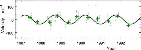
Figure 12. Sinusoidal with a period of 1.52 years is overlaid on the McMillan et al. (1992) velocity variations. Individual measurements are shown by circles, run means by crosses.
Download figure:
Standard image High-resolution image6. THE THIRD SIGNATURE OF GRANULATION
As described in several previous publications (Paper 1 and references therein), the third signature is a plot of the core depths of spectral lines as a function of the core velocities on an absolute scale. For stars on the cool half of the HR diagram, i.e., those with convective envelopes, granulation pervades the photosphere. Granulation displays the dynamical structure of material being thrown upward by the convection below. This material decelerates, cools, and falls back down. But since the hotter material dominates the light we see, the net affect on spectral lines is a blueshift, larger shifts for weaker lines with cores formed in deeper layers.
For Cyg, 32 lines are sufficiently unblended to use in the third-signature plot. There is no evidence of variation in the shape of the third signature plots from individual exposures. An average was taken over the 53 exposures having reference lamps (Section 3 above), yielding the result shown in Figure 13. The mean rms line-depth error is 0.0016, which introduces negligible error in the third-signature analysis. Similarly the mean velocity error is 12 m s−1, making it clear that the apparent scatter of the points in Figure 13 arises from line blends and errors in absolute wavelengths. The "tails" on the points are based on line bisector points taken at 70% of the central line depth. Normal unblended lines will show a small tail arising from the C shape of the bisector, but larger tails are a measure of how badly the line is blended. The tails in this diagram indicate the direction and approximate velocity shift the point can be expected to move if it were not blended. (This convention is opposite the one used in Paper 1.)
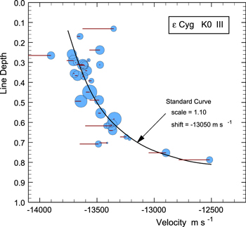
Figure 13. Third-signature plot for Cyg. Symbol diameter varies inversely with the observed scatter relative to each exposure mean. Tails are a measure of the line asymmetry. Large tails indicate blends and a rough estimate of where the line core position would be without the blend.
Download figure:
Standard image High-resolution imageThe standard curve (Gray 2009), anchored to the Sun, is shown scaled up in velocity by 1.1 ± 0.1 times and shifted by −13050 ± 40 m s−1. In addition, the zero point of the standard curve is uncertain by ∼50 m s−1. The mean time associated with these values is 2005.6597 or JD-2450000 = 3610.5272. The scaling factor implies that the granulation velocities in Cyg are 10% larger than in the solar photosphere. This is typical of K giants. In fact, a scale factor of 1.1 with a value of  = 4.45, places Cyg right on the class III line in Figure 8 of Gray & Pugh (2012). In contrast, the scale factor for β Gem (Paper 1) is only 0.8, which might be connected to it being somewhat lower in the HR diagram.
The full range of differential velocities through the whole photosphere is ∼1000 m s−1. Since the top-most photospheric layers have near zero velocities, the granulation rise velocities at the bottom of the photosphere are ∼1000 m s−1. The true rise velocities, allowing for the disk integration, are a few per cent larger.
Classical radial velocity measurements are systematically in error owing to the granulation blueshifts (Bray & Loughhead 1978; Dravins 2008; Gray 2009). In fact, it is clear from the very existence of the third signature that radial velocities deduced using classical methods depend on the combination of line strengths being used. By contrast, radial velocities derived from third-signature plots are freed of these systematic errors. The average velocity for the lines in the third-signature plot for Cyg is 426 m s−1 more negative than the true value, which gives some indication of the size of inherent systematic errors involved in classical radial velocity measurements. It is the blueshift-corrected value of −13050 m s−1 that should be compared with other spectroscopic determinations, while the true space velocity is found by also allowing for the gravitational redshift. If the mass of Cyg is two solar masses and the radius is 11.1 solar radii, the redshift is ∼114 m s−1, yielding a true radial velocity of −13164 m s−1.
7. FLUX DEFICIT AND GRANULATION CONTRAST FROM BISECTOR MAPPING
The mean bisector of Fe i λ6253 for Cyg shows a typical "C" shape (Gray 2005a) and lies between the bisectors of η Dra and α Ari shown in Figure 8 of Paper 1, only slightly different from the β Gem bisector shown there. The deviations of bisectors from the third-signature plot are interpreted as a result of the imbalance between flux coming from the granules compared to the dark lanes. A more complete formulation can be found in Gray (2010a) and Paper 1. The observed imbalance is expressed as a flux deficit that is found by mapping the λ6253 bisector on to the third-signature curve for the star by raising the right side of the line profile. The results for Cyg are shown in Figures 14 and 15. The flux deficit in Figure 15 has been normalized to the depth of the line core, which has a value of 0.763. The size and shape of the Cyg deficit is essentially identical to that of η Dra shown in Figure 13 of Paper 1. Peaking 4.9 km s−1 redward of the line core, it reaches a maximum of 0.165 ± 0.005 or 16.5% ± 0.5% of the profile depth. Its area, normalized to half the equivalent width of the line, is 14% ± 1%. These values agree well with previous determinations for other stars when deficit area is plotted as a function of absolute magnitude or third-signature scale factor, as summarized in Figure 12 of Paper 1.
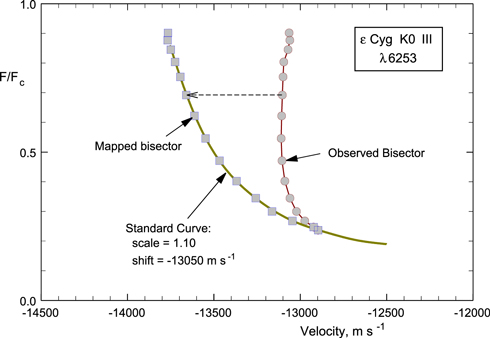
Figure 14. Mean observed bisector is mapped into the scaled third-signature relation from Figure 13.
Download figure:
Standard image High-resolution image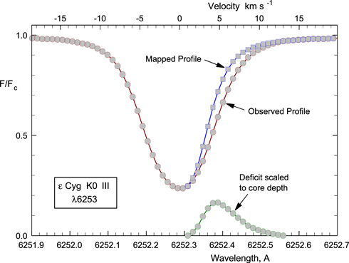
Figure 15. Mapping process with the line profile. The deficit shown is the difference between the mapped and observed profiles divided by the core depth.
Download figure:
Standard image High-resolution imageThe temperature difference between granules and lanes for Cyg, using the same assumptions as in Gray (2010a) and Paper 1, most importantly equal areas for granules and lanes, or equivalently that all the contrast arises from temperature differences, is 145 K. This is larger than the 122 K found in Paper 1 for β Gem, also a K0 III, and within error of the solar value (Gray 2010a).
8. SUMMARY
A detailed analysis of 12 seasons, 1999–2010, of spectroscopic data for Cyg taken with the coudé spectrograph at the Elginfield Observatory yields
- (1)53 new radial velocities placed on an absolute scale with convective blueshifts removed, which help define the 55-year orbit;
- (2)line-depth ratios showing a systematic rise and fall in temperature amounting to ∼4 K, probably arising from a magnetic cycle;
- (3)a possible velocity variation, ∼100 m s−1, mimicking the temperature variation;
- (4)line-broadening parameters, deduced from Fourier analysis, of projected rotation rate v sin i = 1.0 ± 0.2 and macroturbulence dispersion
 = 4.45 ± 0.05 km s−1;
 - (5)a possible rotational modulation seen in the residual velocities with a period of 1.52 years;
- (6)a third signature of granulation with a velocity scale 1.1 ± 0.1 larger than the Sun's;
- (7)a typical bisector shape, and a flux deficit (a measure of granulation contrast) that is consistent in strength and velocity positioning with previously measured K giants and indicates a granule-dark-lane temperature difference ∼145 K.

I am grateful to the Natural Sciences and Engineering Research Council of Canada for funding. I thank M. Debruyne for observatory support and various student observers who, over the years, helped collect some of the observations.