


ABSTRACT
An emerging paradigm for the dissipation of magnetic turbulence in the supersonic solar wind is via localized small-scale reconnection processes, essentially between quasi-2D interacting magnetic islands. Charged particles trapped in merging magnetic islands can be accelerated by the electric field generated by magnetic island merging and the contraction of magnetic islands. We derive a gyrophase-averaged transport equation for particles experiencing pitch-angle scattering and energization in a super-Alfvénic flowing plasma experiencing multiple small-scale reconnection events. A simpler advection–diffusion transport equation for a nearly isotropic particle distribution is derived. The dominant charged particle energization processes are (1) the electric field induced by quasi-2D magnetic island merging and (2) magnetic island contraction. The magnetic island topology ensures that charged particles are trapped in regions where they experience repeated interactions with the induced electric field or contracting magnetic islands. Steady-state solutions of the isotropic transport equation with only the induced electric field and a fixed source yield a power-law spectrum for the accelerated particles with index α = −(3 + MA)/2, where MA is the Alfvén Mach number. Considering only magnetic island contraction yields power-law-like solutions with index −3(1 + τc/(8τdiff)), where τc/τdiff is the ratio of timescales between magnetic island contraction and charged particle diffusion. The general solution is a power-law-like solution with an index that depends on the Alfvén Mach number and the timescale ratio τdiff/τc. Observed power-law distributions of energetic particles observed in the quiet supersonic solar wind at 1 AU may be a consequence of particle acceleration associated with dissipative small-scale reconnection processes in a turbulent plasma, including the widely reported c−5 (c particle speed) spectra observed by Fisk & Gloeckler and Mewaldt et al.
Export citation and abstract BibTeX RIS
1. INTRODUCTION
Magnetic reconnection has been widely invoked to explain the energization of ions and electrons throughout the heliosphere, from solar flares and Earth's magnetosphere (e.g., Drake et al. 2006a; Oka et al. 2010; Birn et al. 2012; Cargill et al. 2006, 2012 and references therein) to even the heliopause (Lazarian & Opher 2009). An interesting series of studies has also considered particle energization in astrophysical flows, identifying related first- and second-order Fermi acceleration-like mechanisms due to magnetic reconnection (de Gouveia dal Pino & Lazarian 2005; Kowal et al. 2011, 2012). Despite the wide application of some form or another of reconnection mechanisms to a variety of heliospheric and astrophysical environments, the precise physical mechanism by which magnetic reconnection energizes charged particles is still not fully understood. Typically, particle acceleration within reconnecting current sheets has been invoked because this can generate direct current (DC) electric fields that accelerate (or decelerate) charged particles. The idea that a statistical acceleration mechanism related to magnetic reconnection was responsible for accelerating particles to high energies was first advanced quantitatively by Matthaeus et al. (1984) and Ambrosiano et al. (1988). They investigated the effect of turbulence on particle acceleration in an MHD field by computing test particle trajectories in turbulent MHD reconnecting fields, examining the acceleration mechanism in some detail. Matthaeus et al. (1984) and Ambrosiano et al. (1988) found that turbulence influences the acceleration in two ways. It enhances the reconnection electric field while producing a stochastic electric field that gives rise to momentum diffusion; and it produces magnetic "bubbles" and other irregularities that can temporarily trap test particles in the strong reconnection electric field for times comparable to the magnetofluid characteristic time. A power-law distribution for the energetic particle distribution was found from their test particle simulations.
Here we consider the acceleration of particles assuming an emerging paradigm for the dissipation of magnetic turbulence via localized small-scale reconnection processes. We examine the physics of magnetic island merging and include this statistically in deriving a transport equation for particles experiencing energization in a "sea" of dynamically interacting magnetic islands embedded in a super-Alfvénic flow such as the supersonic solar wind. We solve the transport equation for an incompressible background flow and show that the accelerated particle distribution is a power law in particle speed c. The spectral index of the power-law distribution is found to depend on the Alfvén Mach number, the characteristic diffusion time of charged particles, and the characteristic time for magnetic island contraction.
Below, we discuss reconnection in a turbulent magnetofluid with magnetic island merging. Two forms of the transport equation for particles experiencing pitch-angle scattering and interacting with reconnecting magnetic islands are derived; the first, a gyrophase-averaged transport equation appropriate to nonisotropic particle distributions and a second that assumes near isotropy of the particles, which yields a simpler transport equation. The isotropic 1D form of the transport equation is solved in the steady-state for an incompressible flow.
2. MULTIPLE RECONNECTION AND DISSIPATION IN THE TURBULENT SOLAR WIND
2.1. Simulations of Multiple Magnetic Islands, Reconnection, and Turbulence
The possibility that local reconnection is a primary dissipation mechanism in the solar corona and supersonic wind is attracting considerable attention theoretically and observationally. The dissipation of magnetohydrodynamic (MHD) turbulence by localized reconnection processes suggests the existence of an important 2D (with respect to a large-scale magnetic guide field) component of solar wind turbulence—a possibility that was already suggested from observations by Matthaeus et al. (1990) and Bieber et al. (1996) and on the basis of theoretical models of nearly incompressible MHD (Zank & Matthaeus 1992, 1993), which proposed that solar wind turbulence was of a composite slab–2D character. Although the potential importance of reconnection in MHD turbulence has long been recognized (Matthaeus & Montgomery 1980; Matthaeus & Lamkin 1986; Carbone et al. 1990; Malara et al. 1992; Veltri 1999; Lazarian & Vishniac 1999), both in terms of dissipation on small scales and in its effect on large-scale structures, only recently have detailed quantitative studies of reconnection in turbulence been considered in simulations (Servidio et al. 2009, 2010, 2011) and observationally (Greco et al. 2008, 2009a, 2009b; Osman et al. 2011). This work suggests that multiple reconnection events are intrinsic to and pervasive in magnetized turbulence.
Inhomogeneous magnetic structures or discontinuities are common in the supersonic solar wind (Burlaga 1968; Tsurutani & Smith 1979; Neugebauer 2006) and have typically been identified as narrow noninteracting convected or propagating discontinuities or as boundaries separating flux tubes (Borovsky 2008; Li 2007, 2008). However, current sheets are coherent structures known to be generated dynamically by turbulence (Matthaeus & Montgomery 1980; Matthaeus & Lamkin 1986; Carbone et al. 1990; Bruno et al. 2001; Dmitruk et al. 2004) and likely to be pervasive and ubiquitous in the turbulent solar wind. If coherent structures such as current sheets are distributed intermittently throughout a turbulent solar wind, then one might expect a corresponding intermittent distribution of locations that exhibit enhanced dissipation (e.g., Vasquez & Hollweg 2001; Sundkvist et al. 2007). Servidio et al. (2009, 2010) present an extensive analysis of 2D MHD turbulence direct numerical simulations at high magnetic and fluid Reynolds numbers. The simulations reveal the ubiquitous presence of incompressible MHD reconnection occurring at x-type neutral points, interspersed densely with a complex dynamical population of magnetic islands. The reconnection events are driven by the stochastic complex dynamics of the nonlinear cascade of energy across all scales. The Servidio et al. (2009, 2010) simulations show that the turbulence evolves to a complex pattern of multiscale magnetic islands, possessing an extended distribution of sizes. Like the size distribution of interacting islands, so too are the reconnection rates distributed broadly. Servidio et al. find that rapid reconnection occurs in association with intermittent non-Gaussian current structures. Observational studies by Greco et al. (2008, 2009a, 2009b) find a close correspondence between the distribution of solar wind discontinuities at inertial range scales with the distribution of non-Gaussian structures derived from simulations of strong MHD turbulence. Osman et al. (2011) subsequently associated coherent structures in the solar wind with enhancements in the electron heat flux and the electron and the ion temperature, indicating that the solar wind is heated inhomogeneously.
The simulations of Servidio et al. (2009, 2010, 2011) assume a 2D geometry (as indeed do most of the simulations that we reference below), and one might question the appropriateness of applying such studies to the 3D solar wind. Although there are theoretical (Zank & Matthaeus 1992, 1993; Bhattacharjee et al. 1998; Hunana & Zank 2010) and observational (Matthaeus et al. 1990; Bieber et al. 1996) reasons for supposing that turbulence in the supersonic solar wind is a composite of slab and 2D fluctuations, numerical simulations of 3D compressible MHD turbulence by Dmitruk et al. (2004) provide some support for the 2D perspective. Dmitruk et al. consider 3D compressible MHD in the presence of a large-scale DC magnetic field in the z direction and initiate the simulations in a nearly incompressible regime. They find that current sheet structures form along the DC field in the evolving turbulent flow. Magnetic field fluctuations and structures evolve stochastically and resemble 2D reconnecting structures. Dmitruk et al. suggest that the 2D structures can be related to "component reconnection," which, as described by Birn et al. (1989), is the 2D reconnection of the perpendicular component of the magnetic field in the presence of a strong guide field. Consequently, despite the complicated dynamical behavior of the 3D system, the anisotropic structure of MHD fluctuations with a strong guide field (Shebalin et al. 1983; Oughton et al. 1994) is one that has current sheets aligned preferentially along the DC field superimposed on 2D structures and fluctuations.
Kowal et al. (2011) found that parallel particle acceleration in a reconnecting 2D MHD model without a guide field ended at a certain energy threshold. However, they found that particles can continue to increase their parallel speed in a 2D MHD model with a guide field. Most importantly, fully 3D MHD reconnecting models with no guide field exhibited the same trend as 2D models with a guide field in accelerating particles.
2.2. Observations of Magnetic Islands and Merging
Direct observations of magnetic islands (sometimes called flux ropes or flux transfer events) are common in magnetospheric plasmas and are widely regarded as signatures of magnetic reconnection. Reconnecting current sheets are observed in Earth's magnetotail and, as a consequence of the Kelvin–Helmholtz instability, on the flanks of the magnetopause and on the borders of flow vortices (Nykyri & Otto 2004; Eriksson et al. 2009; Moore et al. 2013). Magnetic islands and discontinuities are observed to have multiple scales, in agreement with high-resolution simulations of MHD turbulence (Greco et al. 2010). Small-scale flux ropes are unstable and local, but larger-scale magnetic islands are observed by various spacecraft in Earth's magnetosphere (Moore et al. 2013), allowing for the detailed study of magnetic reconnection and flux rope formation. By contrast, much less is known about the corresponding processes in the solar wind.
Solar wind flux ropes are associated primarily with magnetic clouds inside interplanetary coronal mass ejections (ICMEs). However, Janvier et al. (2014) identified two populations of flux ropes, the first being the familiar large-scale structures associated with magnetic clouds in ICMEs; the second class, however, is not easily classified. Large-scale flux ropes possess a Gaussian-like distribution, whereas small-scale flux ropes with radii <0.1 AU have a power-law distribution. It is possible that the second population consists mainly of flux ropes around reconnecting current sheets in the solar wind. Some case studies of magnetic islands in the vicinity of the heliospheric current sheet have been presented over the past decade (see, e.g., Eastwood et al. 2002; Foullon et al. 2011), but the origin and nature of small-scale magnetic islands in the inner heliosphere remains poorly understood.
In the absence of multiple spacecraft observations, one may utilize the Grad–Shafranov reconstruction technique to determine magnetic field structure. Trenchi et al. (2013) investigated localized magnetic field structures associated with the dropout and modulation of solar energetic particles (SEPs; Mazur et al. 2000). Mazur et al. (2000) and Giacalone et al. (2000) suggested that if SEPs were released impulsively from a small site on the Sun, and the magnetic field correlation length was large, then the turbulent random walk of the interplanetary magnetic field lines would lead to a mixing of field lines that were both connected and not connected to the source region. By flying through connected and unconnected magnetic field lines, a spacecraft would observe regions (flux tubes) filled with and empty of particles, respectively. Ruffolo et al. (2003) offered an interesting alternative explanation for the dropouts, suggesting that these were related to 2D topological structures that develop dynamically in evolving solar wind turbulence, independently of magnetic field motions on the solar surface. Ruffolo et al. (2003) assume a composite 2D–slab turbulence model. Because particles do not diffuse easily off magnetic field lines, those particles injected from a localized source on the Sun onto field lines governed by slab turbulence will experience significant lateral diffusion due to field line wandering (Matthaeus et al. 1995, 2003). By contrast, those magnetic field lines that form quasi-2D structures or coherent small-scale helical filaments will correspond to regions of high SEP flux. To explore these ideas more closely, Trenchi et al. (2013) considered the SEP event of 1999 January 9–10, which exhibited multiple SEP dropouts. Trenchi et al. used a Grad–Shafranov reconstruction technique (Hu & Sonnerup 2001) to determine the local magnetic field topology. They find that the maximum SEP fluxes all coincided with 2D magnetic structures, in a few cases similar to small-scale magnetic flux ropes, while others possess a more complex current sheet-like topology in which several magnetic islands are embedded. The islands had the same chirality and were therefore separated by x points.
Magnetic islands located near current sheets in the solar wind may be a consequence of magnetic reconnection, as was shown from multispacecraft observations (Eriksson et al. (2014)). The heliospheric current sheet (HCS), representing a large-scale extension of the solar magnetic equator, is surrounded by numerous secondary small-scale current sheets separated by magnetic islands, most likely formed by continual reconnection along the HCS plane. Khabarova et al. (2014) present observations showing that medium-scale and small-scale flux ropes or magnetic islands are present in the solar wind, at least in the vicinity of the HCS, and not associated with ICMEs. Furthermore, their observations indicated that the magnetic islands were experiencing an ongoing merging process simultaneously with the local acceleration of particles.
Finally, recent statistical investigations show that reconnection events and current sheets are associated with intervals of intermittent turbulence (Osman et al. 2014). At low heliolatitudes, turbulent processes can dominate around the heliospheric current sheet, with recurrent reconnection observed at least up to several AU.
2.3. Summary of the Simulations and Observations
Several conclusions can be drawn from the discussion above.
- 1.Multiple reconnection is a fundamental dissipative process in an evolving turbulent magnetized plasma, and the turbulent cascade produces a distribution of reconnecting magnetic islands.
- 2.In the presence of a strong guided magnetic field, MHD turbulence is anisotropic and exhibits a quasi-2D character with 2D reconnecting structures. Furthermore, a quasi-2D model with a guide field appears to capture the basic particle acceleration characteristics exhibited in fully 3D reconnecting MHD turbulence.
- 3.The observed statistical properties of magnetic discontinuities in the supersonic solar wind are very similar to distributions derived from MHD turbulence simulations, and, moreover, the nonhomogeneously distributed coherent structures exhibit increases in the electron heat flux and electron and ion temperatures.
- 4.During SEP dropout events, the regions of enhanced SEP flux can be identified with 2D magnetic structures, including current sheet-like topologies with embedded magnetic islands separated by x points.
- 5.Magnetic islands of different scales are observed in Earth's magnetosphere frequently, and medium- and small-scale flux ropes or magnetic islands have been observed in the vicinity of the HCS, possibly while undergoing a merging process.
2.4. Magnetic Island Merging and Particle Energization
Although we have emphasized above that reconnection is intrinsic to MHD turbulence and a natural consequence of the nonlinear cascade process, considerable insight into the interaction and formation of magnetic islands is gained from more typical symmetric, isolated models of reconnection (both kinetic and MHD; e.g., Sato et al. 1982; Ambrosiano et al. 1988; Hoshino et al. 2001; Drake et al. 2005, 2006a; Pritchett 2006, 2008; Oka et al. 2010; Huang & Bhattacharjee 2013). Of particular interest is multimagnetic island coalescence (Finn & Kaw 1977; Pritchett & Wu 1979; Tajima et al. 1987; Pritchett 2007, 2008; Wan et al. 2008; Oka et al. 2010), especially in view of the observations presented above that showed active merging of magnetic islands occurring in the solar wind.
In the context of isolated reconnection simulations, a tearing-mode instability typically generates localized currents and multiple x lines. The tearing-mode instability is not necessary for the formation of multiple islands separated by x points because these arise naturally in freely decaying turbulence—see, e.g., Figure 4 of Servidio et al. (2010). In either case, neighboring islands can be attracted to one another by the Lorentz force. As illustrated in Figure 1, the merging of the two islands introduces a reconnection event, marked by the heavy X.

Figure 1. Local oppositely directed magnetic field (lines with arrows) in neighboring islands experiences reconnection, sometimes called "antireconnection" because the induced electric field is oriented oppositely to the primary reconnection electric field that led to the initial formation of multiple magnetic islands. The X identifies the reconnection as two islands merge, the heavy arrows denote the reconnection outflow direction, and the dashed line is the separatrix. The orientation of the reconnection electric field induced by magnetic island merging is into the page.
Download figure:
Standard image High-resolution imageIn the context of isolated reconnection models, the reconnection due to the merging of magnetic islands is termed "antireconnection" (Pritchett 2008), and the electric field induced by the antireconnection event is opposite in direction to the electric field of the primary reconnection event. Such terminology is of course inappropriate to reconnection associated with island merging in the context of turbulence because there is no "primary reconnection event." Nonetheless, the physics of the island merger is precisely the same for both MHD turbulence simulations and simulations of isolated reconnection, and we will sometimes use the "antireconnection" electric field terminology where its use is unavoidable. As illustrated in Figure 1, the two magnetic islands eventually merge to form a single large island. Illustrated in Figure 2 is a cartoon, drawn from the simulations of Servidio et al. (2009, 2010, 2011), that shows the in-plane magnetic field. A "sea" of different sized magnetic islands is clearly apparent, surrounded by in-plane magnetic field lines. A magnetic field line component orthogonal to the plane depicted in Figure 2, the guide field, is also present. Particles propagate along magnetic field lines, sometimes experiencing trapping in magnetic islands and other times propagating along the guide magnetic field component. In this way, charged particles experience energization by being trapped in and escaping from multiple magnetic islands.

Figure 2. Cartoon of the in-plane magnetic field, based on simulations by Servidio et al. (2009, 2010, 2011) that show the ubiquitous presence of densely packed magnetic islands with a range of different sizes. The magnetic guide field projects out of the plane of the figure.
Download figure:
Standard image High-resolution imageTest particle simulations in a dynamical "sea" of magnetic islands show that particles experience energization, with spectra that frequently resemble a power law. Three processes essentially govern the gain in energy that a particle experiences. The first, discussed by Drake et al. (2006a), is based on the idea that magnetic islands formed during magnetic reconnection will contract. Particles trapped within the collapsing island experience repeated reflections at the ends of converging mirrors, gaining energy in a first-order Fermi manner (Drake et al. 2006a). PIC simulations presented by Oka et al. (2010) showed that magnetic islands could "oscillate" or " bounce," i.e., undergo both contraction and expansion. Particles trapped in an oscillating island may experience a second-order Fermi energization. A second process for particle energization is also related to the shortening of the magnetic island field line length but is due now to the merging of two adjacent islands. The merged magnetic field lines (Figure 1) shorten as the merging progresses. The contraction of the magnetic field leads to an increase in the particle velocity component parallel to the local magnetic field and a decrease in the perpendicular energy. By sampling multiple merging magnetic islands, particles can be energized via a second-order Fermi process (Drake et al. 2013). A third energization mechanism is discussed by Oka et al. (2010). In this case, particles trapped in a merging magnetic island (Figure 1) can experience multiple interactions with the reconnection electric field generated by the merging of two islands. This is quite distinct from the usual energization of particles by an electric field generated by the reconnection of two long antiparallel magnetic field lines. Unlike the usual particle energization process via reconnection, particles trapped in a merging magnetic island experience an extended period of interaction with the reconnection electric field, and thus significant energy gain is possible (Oka et al. 2010; Pritchett 2008; Tanaka et al. 2010). The test particle simulations of Oka et al. (2010) suggest that this third energization mechanism may be the dominant energization process for particles in reconnection layers.
In this paper, we adopt the emerging paradigm that turbulence in the supersonic solar wind is dissipated via quasi-2D coherent structures or magnetic islands that are created through dynamical processes. The islands interact nonlinearly, merge, contract, stretch, and attract and repel one another. We will consider the three processes above that have been identified as particle energization mechanisms related to the merging of magnetic islands, i.e., magnetic island contraction, magnetic field shortening due to merging, and the antireconnection electric field.
We therefore hypothesize that medium- and small-scale magnetic islands exist throughout the solar wind, probably as the end-point of turbulent processes, and that they experience multiple mergers. In the process of merging, particles are trapped within the dynamically evolving islands. Charged particles gain energy via magnetic island contraction, merging, or repeated interactions with the electric field induced by the merging process itself. Some particles gain energy, and others lose energy. We will show that the accelerated particle distribution is essentially a power law with an index determined by the Alfvén Mach number and the microphysical timescales associated with magnetic island contraction and charged particle diffusion.
3. TRANSPORT EQUATION
A charged particle propagating through a sea of dynamically interacting magnetic islands (Figure 2) surrounded by magnetic field lines will experience a total force

where FL denotes the usual Lorentz force, Fc particle acceleration due to island contraction (Drake et al. 2006a), Fm particle energization due to island merging (magnetic field line shortening) (Drake et al. 2013), and FE is the particle acceleration due to energization by the reconnection electric fields induced by magnetic island coalescence or other events. Here FL = q(E + v × B), and q and m denote particle charge and mass, respectively, v is the (nonrelativistic) particle velocity, E is the large-scale or mean electric field, and B the large-scale or mean magnetic field vector.
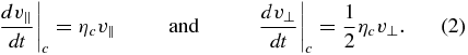
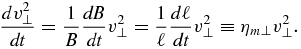
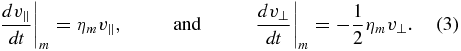
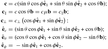
Consider first the acceleration term due to magnetic island contraction Fc = m.dv/dt|c. Drake et al. (2006a) show the trajectory of a charged particle trapped in a contracting island (their Figure 2). Particularly revealing are Figures 2(b) and (c) of Drake et al. (2006a), which show that the trapped particle gains energy in a monotonic manner, with increases occurring at the converging island ends. These figures illustrate very clearly that the process of energy gain is a standard first-order Fermi process. The acceleration term is most simply understood on the basis of the conservation of the first and second adiabatic invariants. Because parallel action is constant, i.e., ∫v∥dℓ' = const., where ℓ' is the field line length, we have ∫v∥dℓ' ∼ v∥ℓ ∼ const. on assuming a characteristic length scale ℓ for an island. This therefore yields
For field line shortening, dℓ/dt < 0 and thus ηc∥ > 0, implying that the parallel velocity increases in time during magnetic island contraction. Conservation of the first adiabatic invariant  shows that
Because the island is contracting, dB/dt > 0, and so the perpendicular energy increases in time as the magnetic island contracts. Recall that for a 2D magnetic island, the magnetic field decreases with radial distance as B = Ψ(r)/r, where Ψ(r) is the magnetic flux,4 so that for a characteristic island size, Ψ ∼ Bℓ. The contracting island flux is constant so that
from which we infer that
For a contracting island, we therefore obtain the acceleration terms (Drake et al. 2006a, 2013)
The island contracts at a speed V = dℓ/dt. Dimensionally, the rate of energy gain due to conservation of longitudinal action is then simply ηc = −αV/ℓ, where the coefficient α is taken to be the ratio of the reconnecting magnetic island magnetic field energy density to the total magnetic energy density, i.e., b2/B2 (Drake et al. 2006a, 2013; Bian & Kontar 2013). A characteristic speed of contraction is V ∼ VA, the local Alfvén speed. Of course, if the magnetic island is expanding, a particle will lose energy at the corresponding rate. If contraction is favored, a particle will experience a gain in energy. Bian & Kontar (2013) use an identical argument, identifying ηc as proportional to the mean compression associated with an average over the ensemble of magnetic islands in the region of interest.
Consider now magnetic island merging (Figure 1) while neglecting the induced antireconnection electric field. Here we follow the analysis of Fermo et al. (2012) and Drake et al. (2013). On crudely approximating the merged island as a circle, we assume that the merging of two islands of initial areas A1 and A2 yields a single island of area A = A1 + A2 = const. Thus, the merged island scales according to  . Again, we assume that the first and second adiabatic invariants hold, so that for an island of characteristic magnetic field line length ℓ,
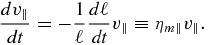
Because the island area is assumed constant,  , implies that the characteristic length ℓ decreases with merging, or dℓ/dt < 0. The second assumption is that magnetic flux is constant (because reconnection simply changes magnetic connectivity, and the flux will be the larger of the fluxes in the two initial islands). Thus, combining the constant area of the merged island A ∼ 2πrℓ with the constant flux Ψ ≃ B2πr yields
Consequently, during island merging, the perpendicular particle energy changes according to
Thus, ηm∥ = −ηm⊥ ≡ ηm, and the particle acceleration terms for merging islands (neglecting the induced antireconnection electric field) become (Drake et al. 2013)
In this case, a particle gains in parallel energy and loses in perpendicular energy.
Denote the fluctuating reconnection electric field by δE' and regard this as a perturbation on the electric field E measured in the stationary frame. We can therefore write

Note that the characteristic timescale for the existence of the fluctuating reconnection electric field for a characteristic island size ℓ and Alfvén speed VA is τE ∼ ℓ/VA, yielding  for a typical individual event.
We begin with the 6D Liouville equation and assume that fluctuating magnetic fields define a scattering term δf/δt)s and then rewrite the equation in the Vlasov form. The acceleration term is separated into two parts, one corresponding to the usual Lorentz electromagnetic force term FL associated with the large-scale fields and the other to energization by coalescing magnetic islands, as discussed above. In principle, all electric fields generated by reconnection processes are included but in dissipative turbulence; this amounts to electric fields induced by magnetic islands. We restrict our attention to nonrelativistic particles for the present. We therefore have
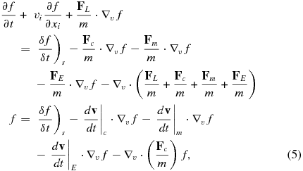
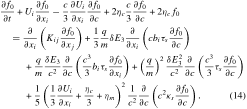
where ∇v is the gradient operator with respect to the particle velocity. Ordinarily, the velocity divergence terms on the right-hand side of Equation (5) are absent in the Vlasov equation because (typically) the force terms are independent of the particle velocity (except the Lorentz term v × B for which ∇v · (v × B) = 0). However, both Fc/m = ηc(v∥, v⊥/2) and Fc/m = ηc(v∥, −v⊥/2) are functions of particle velocity, for which ∇v · Fc/m = 2ηc and ∇v · Fm/m = ηm − ηm = 0.
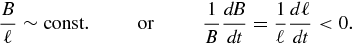
Our purpose is to derive an equation that describes the transport of charged particles in a region of characteristic size L that is much larger than the characteristic size of magnetic islands, i.e., L ≫ ℓ, with a timescale characterized by the large-scale super-Alfvénic flow velocity U within which the reconnecting region is embedded. Consequently, the characteristic timescale for the system is T ∼ L/U. If we normalize Equation (5) with respect to the transport time and length scales and suppose that the characteristic pitch-angle scattering time is ∼τs and the characteristic fluctuating merging magnetic island timescale is τc, m, E ∼ ℓ/VA, then it is straightforward to see that the scattering term is proportional to T/τs, and the merging terms are proportional to T/τc, m, E ∼ (VA/U)(L/ℓ). Because T ≪ τs and L ≪ ℓ, both terms on the right-hand side of Equation (5) may justifiably be regarded as O(1/ε), where ε(≪ 1) is the measure of the ratio of the scattering, contracting, merging, or fluctuating reconnection electric field timescale to the transport timescale. The right-hand side can therefore be separated from the slowly varying left-hand side.
In the absence of an applied electric field, E = −U × B is the motional electric field associated with the large-scale flowing plasma. To eliminate the electric field and move into the frame that ensures that particle scattering does not result in momentum or energy changes, we transform to the flow frame and rewrite v = c + U or c = v − U. We further assume that the flow is super-Alfvénic, specifically, that U ≫ VA, VA the Alfvén speed. In principle, we could alternatively assume that the cross-helicity of the background turbulent fluctuations responsible for scattering the particles is zero. In either case, we can avoid boosting to the background flow plus Alfvén speed. Consequently, the transport equation below is appropriate only to the super-Alfvénic solar wind and not to the sub-Alfvénic regions such as low in the solar corona. For simplicity, we assume that flow accelerations are absent in the large-scale flow field. The transformation of Equation (5) to the plasma flow frame then yields immediately
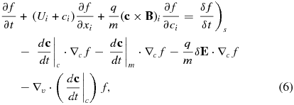
where δE is the induced electric field in the moving frame. Because we are not interested in the gyromotion of the particles, we gyrophase average Equation (6), making the assumption that f(x, t, c, μ, ϕ) ≃ f(x, t, c, μ), where μ = cos θ is the cosine of the particle pitch angle.
Let b ≡ B/|B| and introduce the Cartesian basis set  . The magnetic field, no matter how complex, defines the z or
  coordinate through the directional vector b. δE3 is the corresponding electric field fluctuation in this direction. The gradient operator is given by
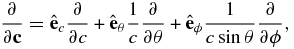
where
The expressions for energy gain in a contracting magnetic island, Equation (2), can then be written as
where 〈⋅⋅⋅〉ϕ denotes an average over gyrophase. We therefore obtain
Similarly, the merging magnetic island energization terms can be expressed as
Finally, the fluctuating electric field δE term, expressed in terms of the Cartesian basis  becomes, after gyrophase averaging,
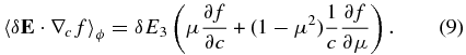
Gyrophase averaging will obviously eliminate particle energization by the fluctuating electric field components orthogonal to the b direction because the gain and loss of energy as the particle gyrates will gyrophase average to zero. Consequently, only δE3 defined by the magnetic field direction can contribute to the energy gain or loss of the particle.
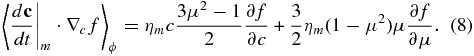
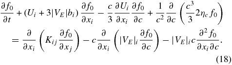
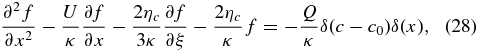
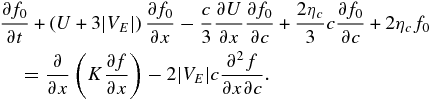
The gyrophase averaging of the left-hand side of Equation (6) proceeds in the usual way (Skilling 1975; Isenberg 1997; le Roux et al. 2007; Webb et al. 2009; see Zank 2013 for details). Including the magnetic island energization terms then yields
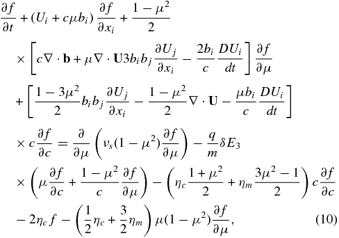
where we have assumed the simplest possible diffusion form for the pitch-angle scattering term

νs = 1/τs, and τs ≃ Ω is a characteristic pitch-angle scattering time, Ω = eB/m, the particle gyrofrequency. Here, D/Dt ≡ ∂/∂t + Uj∂/∂xj is the convective derivative. The gyrophase-averaged Equation (10) describes the transport of energetic particles experiencing pitch-angle scattering in a turbulent plasma embedded with merging and contracting magnetic islands. The distribution function f(x, v, μ, t) is gyrotropic but not isotropic. Equation (10) therefore allows for the description of arbitrarily anisotropic distributions, including beams, etc. Such a description will undoubtedly be important in considering the possible development of firehose or Weibel instabilities, as suggested by Drake et al. (2006b, 2010); Schoeffler et al. (2011), in the reconnection regions due to the energization of particles. Several points about the gyrophase-averaged Equation (10) are noteworthy. Two particle energization terms are present (i.e., ∝c∂f/∂c), one due to the divergence of the large-scale flow velocity, ∇ · U, which is the familiar term responsible for the energization of particles at shocks, and the other due to magnetic island contraction (ηc) and magnetic field line shortening due to island merging (ηm). Notice the close correspondence between the ∇ · U and the contracting island terms. Both enter as first-order terms proportional to (1 − μ2)/2, the first describing the convergence of the bulk flow on the timescale L/U and the latter the convergence/contraction of an island on the timescale ℓ/VA. By contrast, the energization term associated with magnetic island merging has the coefficient
which is proportional to the second-order Legendre polynomial. This indicates immediately that energization via island merging (neglecting for the present the role of the antireconnection electric field) will yield only second-order Fermi energization, in agreement with the result of Drake et al. (2013). Physically, it is clear that assuming conservation of adiabatic moment within the contracting magnetic island will simply redistribute energy between the parallel and perpendicular components. Bian & Kontar (2013) arrive at a similar conclusion although via a quite different approach.
Numerous simulations of test particle energization in reconnecting current sheets yield particle distributions that are essentially isotropic. We invoke this assumption and consider the Legendre polynomial expansion of the gyrophase-averaged Equation (10). This allows us to derive a simpler transport equation analogous to the energetic particle transport equation used in, e.g., cosmic ray investigations. Accordingly, we expand the gyrophase-averaged particle distribution function f as

Following the derivation in Zank (2013) and neglecting flow shear and acceleration terms yields an infinite set of partial differential equations in the coefficients fn of the Legendre polynomials. The expression is lengthy (Equation (A1)), and we relegate a sketch of the derivation and the fully expanded equation to the Appendix. Applying the Legendre polynomial expansion to the electric field term on the right-hand side of Equation (10) yields
The third term on the right-hand side of Equation (10) maps to
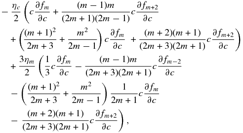
and the final two terms map to
The full set of infinite partial differential equations corresponding to the Legendre expansion of the gyrophase-averaged Equation (10) is given by Equation (A1) in the Appendix, including the above terms.
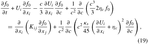
To include the possible effects of second-order Fermi energization in a reduced model describing a nearly isotropic distribution function, we need to consider the f2 approximation (i.e., consider m = 0, 1, 2 or f0, f1, f2 ≠ 0 and fn = 0 ∀ n ⩾ 3). For simplicity, we henceforth neglect the shear terms ∂Uj/∂xi and convective derivatives DUi/Dt—these are easily if tediously incorporated.
The m = 0 expansion yields
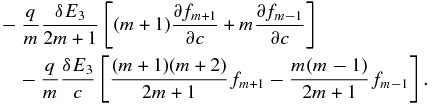
which shows explicitly the important result that island contraction yields a first-order energization term for the isotropic or zeroth-order distribution function f0 proportional to (c/3)∂f0/∂c. The first of the energization terms is familiar from the transport of cosmic rays and describes energy gain or loss due to a compressive or divergent large-scale flow field (e.g., diffusive shock acceleration). The second energization term on the left results from contracting magnetic islands. The right-hand side of Equation (11) contains the higher-order moments of the expansion, f1 and f2. To compute these terms, subject to the closure assumption that fm = 0 ∀ m ⩾ 3, we need to consider the next-order expansions. On considering the m = 1 terms, we find
By assuming that f1 ≪ f0 and f2 ≪ f0 and that the scattering frequency νs = (τs)−1 is large (fast scattering), we obtain the approximate result
Thus, the first-order correction may be approximated by (1) the diffusion description (as is well known, and the spatial diffusion coefficient is proportional to the particle scattering frequency νs and independent of the reconnection terms) and (2) the induced antireconnection electric field energization term.
To obtain the solution for f2, we consider the m = 2 order expansion. The appropriate expansion yields the equation
Again making the assumption of rapid scattering and the subsequent smallness of the higher-order corrections, we find that the approximate solution for f2 is

The first term introduces diffusion in energy due to particle pitch-angle scattering, and the second and third terms are energy diffusion terms due to contracting and merging magnetic islands, respectively. Notice also that the reconnection energization terms also include the effect of particle scattering. Scattering produces two interesting effects for second-order Fermi energization. First, one can obtain second-order Fermi heating from a single island because particle pitch-angle scattering can sometimes scatter particle pitch angles close to 90°, in which case the particle will be lost to the island, and sometimes particle pitch angles will be scattered close to 0°, leading to particle trapping and therefore heating. Multiisland interaction is not therefore a requirement for second-order Fermi heating to occur. Second, in a multiisland context, particle scattering can ensure particle escape and entrance of particles into multiple contracting or merging magnetic islands and therefore facilitates a second-order Fermi energization. Notice also that the antireconnection electric field does not enter at this order.
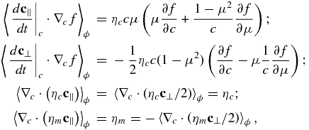
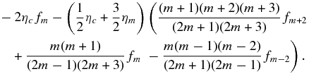
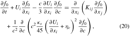
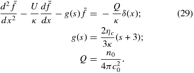
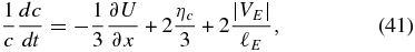
The approximate solutions for f1 and f2 can be used to determine a closed transport equation in f0. Let us introduce the notation
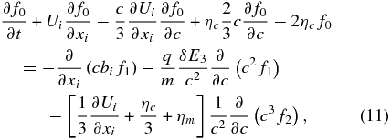
which will describe the spatial diffusion coefficient in the final transport equation. The most general form of the transport equation for a distribution that is close to isotropic is then given by
We can rewrite Equation (14) slightly by introducing a scattered antireconnection electric-field-induced velocity
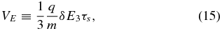
which has a sign dependence because of the charge. We use VEi = −|VE|bi ≡ |VE|i and assume that (q/m)δE3 is independent of x to obtain
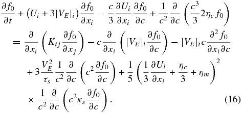
In many respects, the transport Equation (16) is very similar to the standard Parker–Axford–Gleeson transport equation, elaborated further below. Equation (16) illustrates that particles propagating within a region containing dynamically merging magnetic islands and antireconnection electric fields can experience first-order energization or cooling. Related transport equations that include the effects of fluctuating electric fields have been derived previously by le Roux et al. (2002); Kichatinov (1983); Fedorov et al. (1992); Dorman et al. (1987), although not related to the concept of merging magnetic islands.
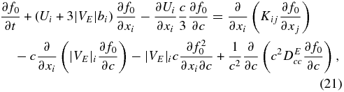
Equation (14) can be rewritten in a particularly revealing and useful phase space conservation form,
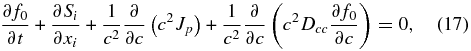
where

is the energetic particle streaming in space,
is the streaming in momentum space, and the diffusion coefficient in velocity space is given by
By estimating δE3 ∼ VAB and introducing a characteristic particle speed c0, we can order the terms in Equation (16) using  . The second and third terms on the right-hand-side scale as
  and
and  , whereas the fourth term scales as
  . Thus, the first-order correct transport equation for
  is
is
Evidently, only island contraction and the induced antireconnection electric field associated with island merging are important for particle energization at the leading order. The transport equation that describes energization by contracting islands alone (i.e., ηc ≠ 0, ηm = 0, δE3 = 0) is given by
where the second term on the right-hand side of Equation (19) describes second-order Fermi energization associated with both the flow divergence and magnetic island contraction. Particle diffusion, expressed through the spatial diffusion coefficient κs enables particles to experience on average more compressive/contraction energy gains than losses. By contrast, in the presence of merging alone (i.e., neglecting both magnetic island contractions ηc = 0 and the antireconnection electric field δE3 = 0), the transport equation reduces to
showing that the reconnection through merging contributes to particle energization only through a second-order Fermi process.
Finally, retaining only the antireconnection electric field and setting ηc = ηm = 0 yields
where
is the second-order velocity diffusion coefficient.
Were we to neglect the second-order Fermi acceleration terms on the right-hand side of Equation (16), the transport equation would be very similar to the standard Gleeson–Axford–Parker transport equation used in the study of cosmic ray transport (e.g., Zank 2013) except for the reconnection terms. Equation (16) illustrates that particles propagating within a region, such as a reconnecting current sheet that produces numerous merging and contracting magnetic islands and antireconnection electric fields, can experience first-order and second-order energization. The second-order energization of particles relies on the presence of scattering (the second Fermi acceleration term is the product of both reconnection and spatial diffusion), which allows the particle to scatter out of an energization region before losing energy.
Finally, we mention that we have also derived the corresponding focused transport equation for relativistic charged particles and its isotropic, advection–diffusion counterpart. The equations are structurally identical except for a relativistic factor in the time derivative and the use of the momentum rather than the velocity variable.
4. PARTICLE ENERGIZATION IN AN INCOMPRESSIBLE FLOW
Let us consider perhaps the simplest of problems: an incompressible super-Alfvénic flow, ∇ · U = 0, with a steady injection of particles of fixed initial speed c0 at the origin, and consider a 1D problem. We further assume for analytic convenience that the spatial diffusion coefficient is constant, and we neglect the second-order energy diffusion terms. We will consider several examples to illustrate the effect of the different energization mechanisms.
4.1. Particle Acceleration by the Antireconnection Electric Field Alone
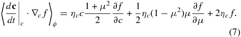
After rearranging (21) slightly and discarding the second-order velocity diffusion term, introducing ξ = ln (c/c0) yields the governing equation as (neglecting the "0" subscript on f0)
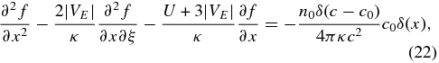
where all the coefficients are constant, including the particle number density n0. The principal part of the differential operator in Equation (22) shows that Equation (22) is hyperbolic with characteristic curves ξ+ = −2(|VE|/κ)x + const. and ξ− = const. To solve (22), we introduce a Laplace transform in the variable ξ, ![$\bar{f} (x,s) = {\cal L} [f(x,\xi)]$](https://content.cld.iop.org/journals/0004-637X/797/1/28/revision1/apj503706ieqn16.gif) , which reduces (22) to the second-order nonhomogeneous ordinary differential equation,
, which reduces (22) to the second-order nonhomogeneous ordinary differential equation,
The complementary solution to Equation (23) is
after demanding  be bounded as x → +∞, assuming that
  as x → −∞, and assuming continuity of
  i.e.,
i.e.,  as ε → 0. The constant A can be obtained by integrating Equation (23) over the interval [ − ε, ε] and taking the limit ε → 0, which yields the jump condition
where [F] ≡ F0 − − F0 +. Evaluating the derivatives across x = 0 yields A = Q/g(s), or
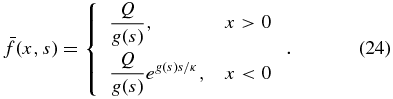
The solution ahead (x < 0) of the particle injection point decays exponentially from the source with a scale length determined essentially by the spatial diffusion coefficient κ and the bulk velocity U and is constant behind (x > 0) the source.
The inversion of  for x > 0 is straightforwardly obtained by the method of residues for the simple pole at s = s0. For x < 0, some care needs to be exercised in choosing the contour in the complex s plane because one needs to ensure the convergence of the integral
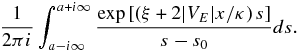
Only if ξ + 2|VE|x/κ > 0 can an enclosed contour containing s0 be chosen, whereas if ξ + 2|VE|x/κ < 0, the closed contour cannot include s0. When the latter condition holds, f(x, c) = 0. The solution for x < 0 is then obtained, yielding the full solution for c > c0 as
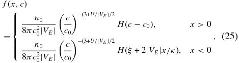
where H(x) is the Heaviside step function. The solution for x < 0 essentially reflects "causality" because recall that ξ + 2|VE|x/κ is one of the characteristic variables of the hyperbolic Equation (22), and the step function implies ln (c/c0) + 2|VE|x/κ > 0. The solution for c > c0 is a simple power law in particle speed. By integrating Equation (25) over c, one can obtain the spatial distribution of the number density n for the energized particles, thus
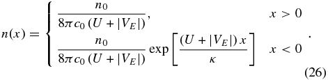
The number density is constant downstream of the particle source and decays exponentially upstream of the source. The latter is the result of particles having to diffuse upstream against the flow.
The solution for c < c0 can be derived directly from the analysis above by noting that defining |ξ| = |ln (c/c0)| yields the same Equation (22) if we use ξ↦|ξ|. The corresponding solution for c < c0 then follows from Equation (25) if we substitute |ln (c/c0)| for ξ. Thus, for particle speeds c < c0, we obtain
which when combined with (25) yields a (logarithmically) triangular particle distribution bounded by two symmetric power laws. The spatial dependence of the number density for cooled particles is similar to that of Equation (26). A sketch of the solution is illustrated in Figure 3. The step function in Equation (27) shows that 2|VE|x/κ > ln (c/c0), illustrating that some particles experience deceleration (cooling) through interacting with the reconnection electric field. This is not surprising because particles can as easily lose energy as gain energy in the presence of a direct electric field for an isotropic distribution of charged particles. This effect is contained in the transport equation that we derived for the case of a nearly isotropic distribution. The power-law solutions (25) and (27) yield the complete solution to the stationary Equation (22), and the normalization constant shows that half of the injected particles are accelerated, and half are decelerated. Thus, in terms of net acceleration, there is none because half the particles are cooled, and the other half are energized symmetrically for an isotropic distribution; there is, however, an accelerated component that has energies greater than c0, and this component admits a power-law distribution for accelerated ions or electrons. Any approach to accelerating particles using a direct electric field, whether simulations, as in Oka et al. (2010), or theoretically, as in this work, must always result in a distribution of heated and cooled particles.

Figure 3. Sketch of the solutions (25), (26), and (27), illustrating the exponential decay of the particle number density n(x) upstream from the source of injected monoenergetic particles and the symmetric logarithmically triangular distribution f(x, c/c0) of accelerated and cooled particles.
Download figure:
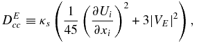
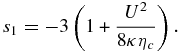
Standard image High-resolution imageThe power-law index can be estimated from
so that the index (3 + U/|VE|)/2 ∼ (3 + MA)/2, where MA = U/VA is the Alfvén Mach number. For Alfvén Mach numbers MA < 5, the spectral index is hard, being less than 4.
4.2. Particle Acceleration by Magnetic Island Contraction Alone
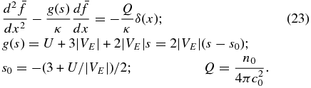
The original discussion of particle acceleration by magnetic island reconnection (Drake et al. 2006a) focused on the effects of magnetic island contraction exclusively. The subsequent numerical simulations by Oka et al. (2010) separated the contributions of the various energization mechanisms associated with particle acceleration. To isolate particle acceleration by magnetic island contraction, we consider the solution of the transport Equation (19), i.e., only ηc ≠ 0, in the limit of an incompressible flow. As with the previous example, we introduce ξ = ln (c/c0) to obtain (neglecting the 0 subscript on f0)
where Q = n0/4πc2. Unlike Equation (22), Equation (28) is strictly parabolic. The Laplace transform in ξ, ![$\bar{f} (x,s) = {\cal L}[f(x,s)]$](https://content.cld.iop.org/journals/0004-637X/797/1/28/revision1/apj503706ieqn22.gif) , yields a second-order linear nonhomogeneous ordinary differential equation,
, yields a second-order linear nonhomogeneous ordinary differential equation,
Equation (29) is solved straightforwardly using the method of variation of parameters. The complementary solutions of Equation (29) are
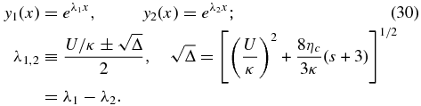
On noting that y1 → 0 and y2 → ∞ as x → −∞, and y1 → ∞ and y2 → 0 as x → ∞, the solution of Equation (29) is given by
or, equivalently,
after expressing  , where
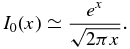
On rewriting (31) slightly, we can use a tabulated Laplace integral transform (Erdélyi et al. 1954, p. 246. formula (6)) to obtain
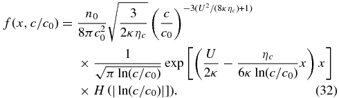
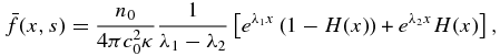
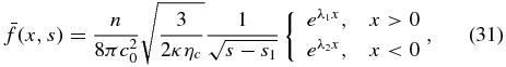
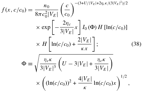
It is instructive to express the solution (32) in terms of the diffusive timescale τdiff ≡ κ/U2, the magnetic island contraction timescale  , and the diffusion length scale Ldiff ≡ κ/U. The distribution function (32) for the accelerated particles then becomes
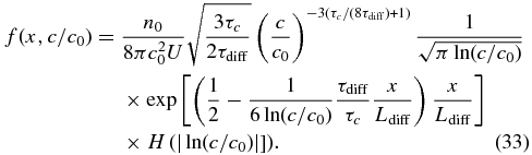
Evidently, solution (33) is essentially a power law for c > c0, which is consistent with the numerous test particle simulations cited above that yield isotropic power-law distribution functions for the energized particles. However, it is apparent that the underlying microphysics of the energization process in contracting magnetic islands and the physics of charged particle pitch-angle scattering plays a critical role in determining the actual power-law exponent. If the characteristic magnetic island contraction time τc ≪ 8τdiff, the power-law spectral index is very hard with f ∼ c−3. Plotted in Figure 4 are several solutions (33), of which the hardest spectrum corresponds to assuming a ratio of τc/τdiff = 0.5 at x/Ldiff = 1. For c > c0, the distribution is essentially a power law with slope ∼−3. Also illustrated in Figure 4 are three examples of the solution to Equation (33) for different choices of the ratio τc/τdiff = 5, 7, 9. These slopes are steeper and correspond to the power-law index of Equation (33).

Figure 4. Plot of the normalized solution (33) for particles accelerated by magnetic island contraction alone. Four curves are plotted, one for a value of τc/τdiff = 0.5 and three for τc/τdiff > 1. For c/c0 > 1, all the solutions are essentially power laws, with the small value of the ratio τc/τdiff yielding a spectral index ∼ − 3. Increasing values of τc/τdiff yield steeper spectra. The solution is normalized to  at the normalized spatial location
  .
.
Download figure:
Standard image High-resolution imagePrecise estimates of both τc and τdiff are beyond the scope of this paper, but order-of-magnitude estimates are possible. We may take τc = (ηc)−1 = ℓ/VA (Drake et al. 2006a; Bian & Kontar 2013; neglecting a possible factor of b2/B2). Considering the relation τc ⩽ 8τdiff or ℓ/VA ⩽ 8c2τs/(3U2) and rewriting τs = λmfp/c, where λmfp is the particle scattering mean free path, yields
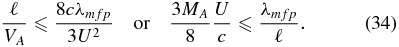
The inequality (34) delineates the conditions under which a relatively hard power-law index (α = −3 to say −5) can be expected. The inequality (34) is easily met for typical quiet-time solar wind conditions because the left-hand side is of O(1). Of course, for particle energization to occur relatively efficiently via the magnetic island contraction mechanism, particle scattering within the island should be relatively weak, and so the condition ℓ ≪ λmfp is implicitly assumed. We note that nonlinear particle feedback effects might well damp the magnetic islands' ability to accelerate particles, leading to a steeper spectrum than suggested here.
Acceleration by the island contraction mechanism can therefore be expected to produce rather hard power-law spectra, as illustrated in Figure 4. However, unlike the induced or antireconnection electric field case above or diffusive shock acceleration, the properties of the power-law solution are not determined from macroscopic flow boundary conditions but rather by the detailed microphysics of charged particle scattering and magnetic island contraction.
4.3. Complete First-order Correct Solution
Having identified the individual contributions of the first-order antireconnection electric field and magnetic island contraction to the energization of particles in regions of reconnecting current sheets, we consider briefly solutions to the full first-order correct steady-state transport Equation (18) for an incompressible flow. The steady-state 1D equation may be expressed as (neglecting the 0 subscript again)
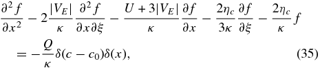
where the various terms have been defined above. Like the anti-reconnection electric field case, Equation (35) is a hyperbolic equation with the same characteristic curves. The discussion of Section 4.1 therefore carries over. We follow the analysis of Section 4.2, Laplace transforming (35) to obtain the second-order, nonhomogeneous linear ordinary differential equation
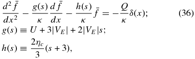
to obtain
By using formula (36), p. 249 of Erdélyi et al. (1954), the inverse Laplace transform of Equation (37) yields the solution
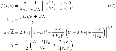
where I0 is the modified Bessel function of order 0. Note again the presence of the characteristic curves ξ+ = −2|VE|/κ + const. and ξ− = const. We do not repeat the discussion about accelerated and cooled particles. Equation (38) describes the particles that have acquired speeds c > c0, and the power-law-like character of the solution is evident. As before, the nature of the solution (38) is most clearly revealed when expressed in terms of characteristic scales and the Alfvén Mach number. Hence
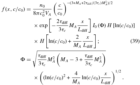
Solutions (39), i.e., for c > c0, are plotted in Figure 5. Figure 5 (top) assumes MA = 7, and Figure 5 (bottom) uses MA = 11, together with the four values of τc/τdiff used in Figure 4. The solutions for both values of MA exhibit power laws for virtually all values of c > c0, and the slope depends on the choice of MA and τc/τdiff. However, it is interesting that the power-law exponent α in Equation (39) for (c/c0)−α does not accurately represent the slope of the solutions plotted in Figure 5. The parameters used in the plot would give an exponent α much steeper than plotted. Instead, the modified Bessel function has a positive slope and contributes to the (c/c0) distribution by flattening the overall slope. The smaller Mach number plots (Figure 5, top) have harder spectra, with power-law exponents ranging from ∼ − 3.2, −3.53, −3.63, to ∼ − 3.7, compared to the higher Mach number plots (Figure 5 bottom), where the exponents now range from ∼ − 3.2, −3.8, and −4, to ∼ − 4.1 for τc/τdiff = 0.5, 5, 7, and 9, respectively. The argument of the modified Bessel's function (39) is large, allowing it to be approximated as
On neglecting the factor of 2π and assuming that aln 2(c/c0) ≫ abln (c/c0), where  ,
,  , b ≡ 4(x/Ldiff)/MA, yields
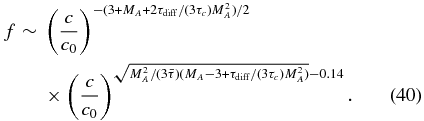
Here the factor 0.14 results from approximating the term  in the range c/c0 ∈ [10, ..., 100]. It is easily verified that the expression (40) yields virtually identical values for the power-law slopes derived from the plots of Figure 5.

Figure 5. Plot of the normalized solution (39) for particles accelerated by the antireconnection electric field and magnetic island contraction. Five curves are plotted, two for values of τc/τdiff < 1 and three for τc/τdiff > 1. (a) These solutions assume that MA = 7, which is possibly appropriate for the inner heliosphere within 1 AU or for periods of solar minimum. (b) These solutions assume that MA = 11, which is possibly appropriate for the outer heliosphere beyond ∼2 AU or for periods of solar maximum. The solution is normalized to  at the normalized spatial location
  .
.
Download figure:
Standard image High-resolution imageThe solutions given in Sections 4.1–4.3 are appropriate only locally in the solar wind because we neglected the divergence term in the transport Equation (18). However, we can estimate quite easily the relative importance of the divergence term compared to the acceleration timescales. The 1D time-dependent transport Equation (18) is simply
If we neglect the spatial diffusion term and introduce a characteristic scale length ℓE so that the last term may be approximated as −2|VE|/ℓEc∂f/∂c, the transport equation may be approximated as a first-order quasi-linear equation. One of the characteristics is then given by
which is the inverse of the particle acceleration timescale. The last two terms are the inverse acceleration timescales due to magnetic island contraction and the antireconnection-induced electric field, respectively. To understand the physical meaning of ℓE, we express the length scale in terms of a timescale that is related to the duration of the magnetic island merging event (because this is the time available to a trapped particle to experience repeated encounters with δE3); thus ℓE ∼ VAτm, where τm is the time taken for the merging of two adjacent magnetic islands. If ℓ is the characteristic size of a magnetic island, then τm ∼ ℓ/VA. Thus, because ηc ∼ VA/ℓ and |VE| ∼ VA, the acceleration rate due to magnetic island merging (both island contraction and induced electric field) is  . We can now compare the size of the particle acceleration rate to that of the expansion or cooling term ∂U/∂x ≃ U/R, where R is the solar wind spatial scale ∼1 AU. If we assume that ℓ is less than the correlation length scale at 1 AU (i.e., ∼0.01 AU), then say
 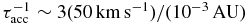 and U/R ∼ (400 km s−1)/(1 AU) implies that the acceleration rate is at least 100 times greater than adiabatic cooling. This justifies our neglecting the divergence term to compute the accelerated particle spectrum.
4.4. The Alfvén Mach Number Throughout the Heliosphere
In view of the central role played by the Alfvén Mach number in the solutions described in Sections 4.1–4.3, in this subsection we present observations describing the variation of the Alfvén Mach number as a function of heliocentric distance and solar activity. In Figure 6, we plot the Alfvén Mach number as a function of heliocentric distance, together with the corresponding value of the spectral index (3 + MA)/2 derived from the induced electric field acceleration example. Specifically, we used hourly data from Helios 2, Pioneer Venus, Orbiter, IMP8, and Voyager 2 for 1976–1979 as described by Khabarova & Obridko (2012), together with Voyager 1 and Helios 1 data sets for the corresponding period. The values were derived as described in http://omniweb.sci.gsfc.nasa.gov/ftpbrowser/bow_derivation.html, taking into account the multispecies content of the solar wind and averaged by distance and all spacecraft. From Figure 6, the Alfvén Mach number is approximately constant beyond ∼1.5 AU with a value of 10–11, yielding a spectral index of ∼6.5–7 for this region. By contrast, the Alfvén Mach number increases from a value of about 5 at 0.3 AU to ∼9 at 1 AU. The corresponding spectral index for the antireconnection case changes from 4 to just less than 6. Of course, the variance, as illustrated by the error bars of Figure 6, can be large. Figure 7 shows that the Alfvén Mach number at 1 AU in the ecliptic plane can vary significantly with solar cycle. During solar maximum, values of MA ∼ 7–8 are common, after which MA increases as the solar minimum approaches (see also Svalgaard & Cliver 2010). Current sheet crossings are associated with plasma characterized by the highest possible Alfvén Mach number because of the abruptly decreasing strength of the interplanetary magnetic field and the enhanced solar wind density. Therefore, even at 1 AU, the corresponding spectral index should reach values typical for the outer heliosphere (and much more) in the vicinity of the heliospheric current sheet.
Figure 6. Plot of the Alfvén Mach number and derived spectral index (3 + MA)/2 for the antireconnection-induced electric-field-alone case as a function of heliocentric distance for the period 1976–1979.
Download figure:
Standard image High-resolution image
Figure 7. Plot of the Alfvén Mach number (top) and sunspot number (bottom) as a function of time through the solar cycle using 27 day averaged OMNI2 data.
Download figure:
Standard image High-resolution imageIt is interesting that if we consider the antireconnection-induced electric field-alone solution (Section 4.1), the roughly constant value of MA in the outer heliosphere between ∼1.5 and 6 AU suggests that f ∼ c−6.5 or c−7 should hold throughout this region during quiet times. It is also intriguing that from about 0.5–1 AU, the value of the Alfvén Mach number yields a spectral index in the range of ∼4–5, or f ∼ c−4–c−5 (Figure 6), which is similar to quiet-time observations of suprathermal (1–50 keV) particle spectra with c−5 reported by Fisk & Gloeckler (2006, 2012) and Mewaldt et al. (2001) for the supersonic solar wind. Similarly, during solar maximum periods at ∼1 AU, MA ∼ 7–8, for which f ∼ c−5–c−6. However, these spectra may be masked in part by particle acceleration due to diffusive shock acceleration during solar maximum. Nonetheless, particle acceleration by reconnection of the kind described here may be useful in providing a seed particle population during this time.
5. CONCLUSIONS
Multiple reconnection has been identified as a primary dissipation process in an evolving turbulent magnetized plasma. Dissipation proceeds through the dynamical interaction of quasi-2D magnetic islands that form a "sea" of coherent structures within which particle energization proceeds. This perspective is supported by both numerical simulations (kinetic and MHD) and observations in the supersonic solar wind. Merging magnetic islands produce a reconnection-induced electric field within a larger closed structure, magnetic islands experience contraction, and magnetic field lines decrease in length during the merging process. Particles trapped in the vicinity of merging islands (Figure 1) repeatedly experience the induced electric field, leading some to gain energy. Particles trapped within contracting magnetic islands gain energy via a first-order Fermi mechanism. Oka et al. (2010) find that the electric field created by magnetic merging is the most effective of the particle mechanisms associated with the merging of magnetic islands. This in part may be due to the possibility that magnetic islands can oscillate rather than uniformly contract. An interesting result that is supportive (but not uniquely definitive) of the idea that magnetic islands might energize particles was obtained by Tessein et al. (2013). Tessein et al. used ACE magnetic field data to identify coherent structures in the solar wind using an approach related to that developed by, e.g., Greco et al. (2009a) and Osman et al. (2011). Using ACE energetic particle data and employing a PVI (partial variance of increments) analysis, Tessein et al. found a strong association of energetic particles in the range 0.047–4.75 MeV with solar wind discontinuities. One possible explanation (although certainly not the only one) is that the particles seen at PVI events were energized locally, possibly by reconnection events.
Khabarova et al. (2014) have presented observations that show the presence of magnetic islands in the vicinity of the heliospheric current sheet. They find that (1) magnetic islands in the solar wind possess a range of spatial scales and (2) magnetic islands experience dynamical merging in the solar wind. This work extends a variety of solar wind observations that support the physical picture described here, viz., one of a turbulent solar wind plasma in which quasi-2D magnetic islands with a range of spatial scales experience multiple reconnection events.
We have derived a transport equation for a gyrotropic distribution of particles experiencing pitch-angle scattering and energization via electric fields generated in a dissipative multireconnection super-Alfvénic plasma. Simulations of particle acceleration in a plasma with multiple reconnection events frequently exhibit isotropic energetic particle distributions. We therefore simplify the gyrophase-averaged or focused transport equation by assuming an isotropic particle distribution. This yields an advection–diffusion transport equation that resembles the well known cosmic ray transport equation except for energization terms due to stochastically distributed reconnection electric fields, contracting magnetic islands, and magnetic field line shortening associated with magnetic island merging.
The total acceleration timescale is given by a balance of the adiabatic term associated with the divergence of the large-scale flow and the magnetic island merging acceleration timescale, i.e.,
where ℓ is a characteristic magnetic island size. At 1 AU, the divergence term can be neglected locally because it is ∼100 times smaller. The acceleration timescale VA/ℓ reflects the time available for trapped particles in merging magnetic islands to either sample repeatedly the reconnection electric field induced by the merging or be trapped in a contracting magnetic island. This is a vital distinction between the time available for charged particles to sample the reconnection electric field induced by the typical reconnection model that is generated by antiparallel magnetic fields in the absence of islands. In the latter case, the acceleration timescale will be determined by Alfvén speed and the reconnection diffusion length scale (distinct from the diffusion scale discussed here in the context of particle transport). Consequently, particle acceleration due to particle trapping in contracting magnetic islands and acceleration in the reconnection electric field induced by island merging is a far more efficient acceleration mechanism than particle acceleration by reconnection electric fields in the absence of magnetic islands.
By considering a simple incompressible background flow, we solved the steady-state isotropic form of the 1D transport equation with a fixed source and injection speed c0. We assumed that the spatial diffusion coefficient was constant and neglected the second-order diffusion terms in energy. We showed that the adiabatic expansion term was some 100 times slower than the particle energization terms associated with reconnecting magnetic islands and could therefore be neglected locally. We considered in some detail the individual contributions to particle energization by the induced electric field and contracting magnetic islands separately. We then solved the first-order correct transport equation with both the electric field and island contraction terms present to obtain the general solution.
The solution for the transport equation in which only the induced or antireconnection electric field energization term is retained yields pure power-law distributions for the accelerated particles, i.e., c > c0, where c0 is the injected initial particle speed. Because the particles experience stochastic encounters with the induced electric field, half the particles are accelerated, and half are cooled. Mathematically, this is expressed through the hyperbolic character of the form of the transport equation in phase space. The half of the injected particles that are accelerated have a power-law distribution with index α = −(3 + U/|VE|)/2, where |VE| is a scattered electric-field-induced velocity (15). A plausible estimate shows that |VE| = VA, yielding a power-law exponent α = −(3 + MA)/2, where MA is the Alfvén Mach number for particle speeds c > c0. The half of the injected particles that lose energy have a power-law spectrum with index α = (3 + MA)/2 for particle speeds c < c0. The full distribution, when plotted logarithmically, therefore has a triangular shape with the apex at c = c0.
The transport equation is strictly parabolic when the energization terms are restricted to magnetic island contraction alone. The accelerated form of the accelerated distribution function is of a power-law-like nature, being a power law for particle speeds c > c0. The power-law exponent α = −3(1 + τc/(8τdiff)) is a function of the magnetic island contraction timescale τc and the particle diffusion timescale τdiff = κ/U2, where U is the large-scale background flow speed. Both of these timescales reflect the microphysics of the island contraction and particle scattering, and neither is particularly well known. If τc < τdiff, then the accelerated particle distribution is very hard, tending to a power-law index α = −3. An inequality was derived, Equation (34), identifying the conditions under which a relatively hard power-law solution can be expected. Under typical quiet-time solar wind conditions, it is only necessary that the particle scattering mean-free path λmfp be larger than the characteristic scale size ℓ of the contracting magnetic island.
Finally, the full first-order correct transport equation was solved when both the induced electric field and the magnetic island contraction energization terms were included. As before, power-law-like solutions were obtained, with the index depending on both the Alfvén Mach number and the ratio τc/τdiff. The value of the approximate power-law exponent is easily estimated for this general case because the exponent is determined primarily by the large argument approximation of the modified Bessel's function component of the solution. We derive a solution for particle speeds c greater than a few c0 that shows the accelerated particle distribution is a power-law-like solution depending on only the Alfvén Mach number and the ratio of the magnetic island contraction scale to the particle diffusion timescale. The combination of induced electric field and magnetic island contraction yields hard spectra for typical parameters. The numerical solutions confirm that the spectra are hard, the flatness being determined by the size of the ratio τc/τdiff for a given Alfvén Mach number. The larger MA implies more efficient escape from acceleration regions and therefore leads to steeper power-law-like solutions for the general case. The governing differential equation was hyperbolic, and therefore many of the characteristics of the electric-field-alone solution were similarly present for this more general case.
Given the importance of the Alfvén Mach number in determining the spectral index or the conditions under which energization via the contracting island mechanism would generate a power law, we presented observations showing the averaged radial dependence of MA for the period 1976–1979 from 0.3–∼6 AU. From 0.3–∼1 AU, MA ranges from ∼5–9, and >1.5 AU, MA ∼ 10–11. In the case of the induced electric-field-alone solution of the transport equation, this yields a predicted power-law spectral index that ranges from −4 to −6 in the inner heliosphere to −6.5 to −7 in the outer heliosphere, varying with solar cycle. At least in the inner heliosphere, this is intriguingly close to the c−5 quiet-time observations of suprathermal (1–50 keV) particle spectra in the supersonic solar wind observed by Fisk & Gloeckler (2006, 2012) and Mewaldt et al. (2001) at 1 AU. These values of MA illustrate that the inequality (34) will be relatively easily met for both the inner and outer heliosphere, so that particle acceleration by island contraction in a reconnecting flow should produce relatively hard spectra. As we showed, the combination of the induced antireconnection electric field and island contraction conspire to generate hard power-law-like solutions of the nearly isotropic form of the transport equation.
Because dissipation via multiple reconnection in a turbulent plasma should also occur in subsonic flows, such as in the lower corona, coronal loops, and the inner heliosheath, it is possible that the mechanism presented here might apply to particle acceleration in these regions. However, the transport equation will need to be rederived to take into account the sub-Alfvénic flow. Finally, we speculate that particle energization through a reconnection mechanism might be applicable to collisionless shock waves. Shocks typically generate significant levels of vortical turbulence downstream, which may therefore be a site for the acceleration of electrons or protons. This may be important for the injection of particles into the diffusive shock acceleration mechanism, or perhaps even partly responsible for the acceleration of particles at collisionless shock waves.
We acknowledge the partial support of NASA grants NNX08AJ33G, Subaward 37102-2, NNX09AG70G, NNX09AG63G, NNX09AJ79G, NNG05EC85C, Subcontract A991132BT, NNX09AP74A, NNX10AE46G, NNX09AW45G, and NNX14AF43G, and NSF grant ATM-0904007. This work was also supported in part by a UAH IIDR award to G.P.Z. O.K. was supported by RFBR grant 14-02-00769. G.P.Z. thanks J. F. Drake, M. Swisdak, W. H. Matthaeus, R. Bruno, and L. Trenchi for useful discussions. G.P.Z. thanks R. Bruno for his kind hospitality while visiting the INAF.
APPENDIX: DERIVATION OF THE ISOTROPIC TRANSPORT EQUATION FROM THE GYROPHASE-AVERAGED TRANSPORT EQUATION
A Legendre polynomial expansion of the gyrophase-averaged Equation (6) can be used to derive a simpler transport equation analogous to that used to describe the transport of cosmic rays. We expand the gyrophase-averaged particle distribution function f as
The orthogonality condition is given by
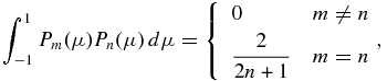
and some useful recurrence relations are
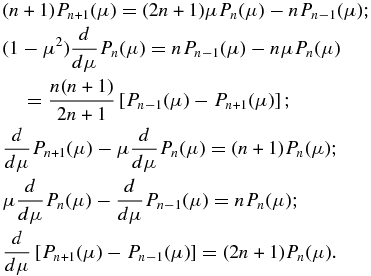
We need
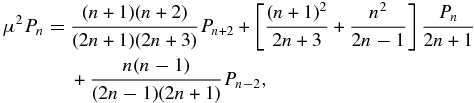
to evaluate
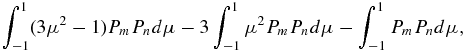
and
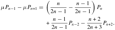
We systematically project and expand each of the terms in Equation (6) from left to right using the Legendre polynomial Pm(μ) and the expansion for f. The left-hand side of Equation (6) and the diffusion in μ term and the additional reconnection terms yield the complete transformed focused transport Equation (6), now, however, expressed as an infinite set of partial differential equations in the coefficients fn of the Legendre polynomials,
The infinite set of partial differential Equations (A1) is equivalent to the focused transport Equation (10) and therefore as challenging to solve. At each order of the expansion, i.e., the partial differential equation for a Legendre coefficient of particular order, it is clearly seen that the equation possesses coefficients of a higher order. This is another expression of the closure problem. Closure is typically affected by simply truncating the Legendre polynomial expansion at a finite number of coefficients. In the body of the text, we consider the m = 1 and m = 2 approximations.
Footnotes
- 4
Consider a magnetic field in the 2D plane perpendicular to the z axis. Thus, ∇⊥ · B⊥ = 0, allowing us to assume
 . Expressed in cylindrical coordinates, , where Br = −(1/r)∂Ψ/∂ϕ and Bϕ = ∂Ψ/∂r for Ψ(r, ϕ). For a circular magnetic island, . Consequently, 〈B⊥〉r = Ψ(r) − Ψ(0).
