


ABSTRACT
We have used precise differential astrometry from the Palomar High-precision Astrometric Search for Exoplanet Systems project and radial-velocity measurements covering a time span of 40 yr to determine the orbital parameters of the 1 Geminorum triple system. We present the first detection of the spectral lines of the third component of the system, together with precise mass (0.5%) and distance (0.15%) determinations for this system. In addition, our astrometry allows us to make the first determination of the mutual inclination of the orbits.
Export citation and abstract BibTeX RIS
1. INTRODUCTION
The star 1 Geminorum (HR 2134, HD 41116, HIP 28734, Kui 23AB) is a bright (mV = 4.15, mK = 2.18), nearby (∼47pc) triple system (Abt & Kallarakal 1963; Tokovinin 1997). Kuiper (1948) made the serendipitous discovery of the A–B close visual binary system, which has an apparent semi-major axis of 0 20 and an orbital period of 13.3 yr. The A component is evolved and has a spectral type of K0III (Abt & Kallarakal 1963), while the B component is a short-period binary system with a 9.60 day period (Griffin & Radford 1976). Strassmeier & Fekel (1990) determined the spectral type of the brighter component of the B system (which we will refer to as Ba) to be F6IV. To our knowledge, no detections of the fainter component, Bb, have been published. Griffin & Radford (1976) and Griffin (1980) have provided the history of earlier work on this bright triple system.
Multiple stellar systems such as 1 Gem are of interest for several reasons. First, it is possible to measure masses of the individual components and the system distance with high precision, while the presence of several stars provides further constraints for stellar models by requiring the binary component stars to be co-eval (Torres & Ribas 2002). That constraint is particularly important in a system such as 1 Gem, where one or more of the components has evolved off the main sequence. Second, as pointed out by Sterzik & Tokovinin (2002), the relative orientations of the orbital angular momenta allow one to constrain the properties of the cloud from which the stars are thought to have formed, as well as the subsequent dynamical decay process, or lack thereof (Tokovinin 2008). Finally, the dynamical interactions of the stars may provide interesting constraints on the magnitude of tidal interactions (Kiseleva et al. 1998; Kiseleva-Eggleton & Eggleton 2001). However, given the often wide range of orbital separations and periods, multiple stars are challenging observational objects that usually require observations by two techniques (imaging and spectroscopy), and so to date only a handful of such systems have been fully characterized (Eggleton & Tokovinin 2008).
Advances in long-baseline stellar interferometry now enable astrometry (Lane & Muterspaugh 2004) with 35 μ-second-of-arc precision and have made it possible to resolve the orbital motion of several interesting multiple systems (Muterspaugh et al. 2006a, 2006b; Lane et al. 2007; Muterspaugh et al. 2008, 2010a). Here we continue this work with a report on astrometry of the 1 Gem system. For the first time we are able to determine the orbital inclination of the close binary system (Ba–Bb), as well as the mutual inclination of the two orbits.
However, astrometry alone is not sufficient to determine fully the orbital and stellar properties of this system. We also present the results of extensive radial-velocity campaigns at various observatories that have followed this system for up to nearly three complete orbital periods of the visual binary. With the combination of our data, which includes 29 Palomar High-precision Astrometric Search for Exoplanet Systems (PHASES) astrometric measurements and 1799 radial velocities, plus 63 high-angular-resolution observations from the literature, we are able to determine fully the system parameters, including masses of the components at the sub-percent level.
Astrometry was obtained for the PHASES program (Muterspaugh et al. 2006c) using the Palomar Testbed Interferometer (PTI; Colavita et al. 1999; Colavita 1999), located on Palomar Mountain. That interferometer operated in the J (1.2 μm), H (1.6 μm), and K (2.2 μm) bands and combined starlight from two out of three available 40 cm apertures. The apertures formed a triangle with 86, 87, and 110 m baselines.
2. OBSERVATIONS AND MODELS
2.1. PHASES Astrometry
1 Gem was successfully observed with PTI on 29 nights in 2004–2007 with the near-IR (2.2 μm) phase-referenced fringe-scanning mode (Lane & Muterspaugh 2004) that was developed for high-precision astrometry. The data were reduced with the use of the algorithms described therein, together with the modifications described in Muterspaugh et al. (2005). In this mode, the primary fringe tracker operated in a high bandwidth phase tracking mode using the highest visibility object in the field of view (the A component) to stabilize the apparent fringe motion introduced by atmospheric turbulence. A second beam combiner measured the fringe patterns produced by all of the components; these fringe data were processed to yield apparent separation angles between the A and Ba–Bb centroids.
Our differential astrometry is listed in Muterspaugh et al. (2010b). Because PTI operated with a single baseline on a given night, the measurement errors are much smaller in the direction aligned with the baseline than they are in the orthogonal direction. To weight the data set properly when doing a combined fit with previous astrometry and radial-velocity data, we have fit an orbital model to the PHASES astrometry by itself. The resulting reduced χ2 was 1.3, indicating a certain amount of excess scatter beyond the internal error estimates. We believe that this scatter is due to systematic noise sources that have been identified in the system (Muterspaugh et al. 2008). After re-scaling the uncertainties by a factor of  , the median minor-axis formal uncertainty is 55 μ seconds of arc, while the median major-axis uncertainty is 250 μ seconds of arc. We also identify two points (MJD 54,029.41661 and 54,376.47755) as outliers, where the nightly data-reduction procedure misidentified the central fringe and calculated a separation that was in error by a factor of λ/B ∼ 4 mas (where λ is the operating wavelength and B is the interferometer baseline); those points were excluded from the subsequent fit.
2.2. Previous Astrometry
In addition to our astrometry, 1 Gem has been followed by a number of observers using speckle-interferometric techniques. We have incorporated 63 observations tabulated in the 4th Catalog of Interferometric Measurements of Binary Stars11 (Hartkopf et al. 2001) to constrain our fit further. Although of somewhat lower precision than our PHASES observations, the considerable time baseline (including observations between 1976 and 2005) of those additional measurements helps to constrain the parameters of the A–B visual binary. In many cases the published astrometry lacks uncertainties, so we derive uncertainties from the scatter of the data about a best-fit simple Keplerian model; we adjust the uncertainties to yield  . We find that the published uncertainties in separation should be increased by a factor of 1.95 and in position angle by a factor of 1.36. For the data points that lack uncertainties we instead assign a value of 3.96 mas in separation and 1.96 deg in position angle.
2.3. Radial Velocity
Extensive radial-velocity measurements of the 1 Gem system have been obtained in four separate campaigns spanning 40 yr, including data from eight different instruments. We describe each data set below.
2.3.1. Palomar, OHP, and Cambridge Observations
Between 1969 and 2009 R.F.G. acquired a total of 128 observations of 1 Gem using the original radial-velocity spectrometer at Cambridge (Griffin 1967, 1980); a second-generation, computerized instrument at Palomar (Griffin & Gunn 1974; Griffin 1980); the CORAVEL spectrometer at Haute Provence Observatory (OHP; Baranne et al. 1979); and, most recently, the Cambridge CORAVEL. The "Cambridge CORAVEL" operates at the Coude focus of the 36 inch reflector on the home site of the Cambridge Observatories, Madingley Road, Cambridge, England. The instrument has not been particularly described in the literature but is broadly patterned after the one described by Baranne et al. (1979). It operates by cross-correlating the spectrum with a mask, a process first developed using a physical rather than a numerical mask on the same 36 inch telescope (Griffin 1967). It uses a mask whose design is based on the spectrum of Arcturus, adopted from the Arcturus Atlas (Griffin 1968).
The radial velocities obtained with the original Cambridge spectrometer and the Palomar spectrometer have been placed on the "Cambridge" zero point, which seems to be 0.8 km s−1 more positive than the zero point favored by the Geneva group (Udry et al. 1999). Velocities acquired with the CORAVEL at Haute Provence have been shifted by +0.8 km s−1 from the values "as reduced in Geneva," while the ones made since 1999 with the Cambridge CORAVEL have been adjusted by −0.1 from the "as reduced" values. The preliminary relative weightings used for computing orbits were 0.1 for "original Cambridge," 0.5 for Palomar and Haute Provence Observatory, and 1 for the Cambridge CORAVEL, except that recent observations (starting from the beginning of 2005) are so much better that they have been given weight 2. We have divided these data into two separate sets in order to allow for different velocity zero points: the Cambridge and Palomar data are referred to as data set A, while the OHP data are labeled set B. The data for components A and Ba are provided in Table 1.
Table 1. 1 Gem Radial-velocity Data Sets A and B (Palomar, OHP, and Cambridge)
| HJD−2,400,000.5 | Velocity (A) | σ | O − C | Velocity (Ba) | σ | O − C | Code |
|---|---|---|---|---|---|---|---|
| (km s−1) | (km s−1) | ||||||
| 40,335.84 | 39.1 | 0.79 | −0.19 | ... | ... | ... | 213 |
| 40,492.22 | 35.6 | 0.79 | 0.11 | ... | ... | ... | 213 |
| 40,494.22 | 33.9 | 0.79 | −1.54 | ... | ... | ... | 213 |
| 40,577.92 | 33.0 | 0.79 | −0.22 | ... | ... | ... | 213 |
| 40,592.90 | 32.8 | 0.79 | −0.03 | ... | ... | ... | 213 |
| 40,986.90 | 22.8 | 0.79 | −1.99 | ... | ... | ... | 213 |
| 41,285.04 | 20.8 | 0.79 | −0.76 | ... | ... | ... | 213 |
| 41,290.10 | 23.0 | 0.79 | 1.47 | ... | ... | ... | 213 |
| 41,639.12 | 19.5 | 0.79 | −0.17 | ... | ... | ... | 213 |
| 41,652.08 | 18.0 | 0.79 | −1.63 | ... | ... | ... | 213 |
Notes. Radial-velocity data for the 1 Gem system from radial-velocity spectrometer observations, the uncertainties, and the fit residuals (O − C values) for the fit. The numbers in the code column of the data set for the respective sources are 213 for "old Cambridge," 218 for Palomar, 313 for the CORAVEL at Haute Provence, and 312 and (post-2005) 412 for Cambridge CORAVEL.
Only a portion of this table is shown here to demonstrate its form and content. A machine-readable version of the full table is available.
Download table as: DataTypeset image
2.3.2. Dominion Astrophysical Observatory Observations and Reductions
A series of observations of 1 Gem has been obtained by C.D.S. with the Dominion Astrophysical Observatory (DAO) radial-velocity spectrometer, in both its original (Fletcher et al. 1982) and subsequent (McClure et al. 1985) configurations. Observations were begun early in 1980 and continued until the end of 2003, shortly before the spectrometer was decommissioned. Masks based on the spectra of Arcturus and Procyon were found to give about equally good results, and all those available have been used at one time or another. Observations of IAU standard stars (Pearce 1957) have been used to adjust the observations made with each mask to the zero point of Scarfe (2010).
The DAO velocities of components A and Ba are listed in Table 2. It was not found necessary to apply corrections for blending, of the kind described by Scarfe et al. (1994), but a few velocities obtained from blended profiles have been rejected and omitted from that table, as have a few others whose residuals from a preliminary solution of the DAO velocities alone were over three times the rms value for the relevant star. The total number of acceptable velocities from DAO radial-velocity scanner observations is 123 of the primary star and 107 of the brighter component of the close pair. The third component was not detectable in the DAO traces. We identify the DAO observations as data set C.
Table 2. 1 Gem Radial-velocity Data Set C (DAO)
| HJD−2,400,000.5 | Velocity (A) | σ | O − C | Velocity (Ba) | σ | O − C |
|---|---|---|---|---|---|---|
| (km s−1) | (km s−1) | |||||
| 44,257.279 | 30.1 | 0.66 | 0.01 | ... | ... | ... |
| 44,291.217 | 31.2 | 0.66 | 0.61 | 74.2 | 1.40 | 1.05 |
| 44,298.200 | 31.4 | 0.66 | 0.71 | ... | ... | ... |
| 44,304.230 | 31.3 | 0.66 | 0.52 | −7.0 | 1.40 | 0.16 |
| 44,321.240 | 30.7 | 0.66 | −0.34 | 61.8 | 1.40 | 1.65 |
| 44,339.146 | 31.0 | 0.66 | −0.32 | 70.4 | 1.40 | −2.05 |
| 44,492.548 | 33.4 | 0.66 | −0.45 | 68.9 | 1.40 | −0.96 |
| 44,548.415 | 34.1 | 0.66 | −0.72 | ... | ... | ... |
| 44,614.297 | 36.4 | 0.66 | 0.41 | −11.6 | 1.40 | 0.31 |
| 44,670.137 | 37.2 | 0.66 | 0.23 | −34.5 | 1.40 | −0.16 |
Notes. Radial-velocity data for the 1 Gem system from DAO, together with the uncertainties and the fit residuals (O − C values) for the fit.
Only a portion of this table is shown here to demonstrate its form and content. A machine-readable version of the full table is available.
Download table as: DataTypeset image
2.3.3. KPNO Observations and Reductions
From 1983 through 2009 F.C.F. obtained observations at the Kitt Peak National Observatory with the 0.9 m coudé feed telescope, coudé spectrograph, and several different CCD detectors. All of the spectrograms were acquired with a Texas Instruments (TI) CCD except for five that were obtained in 1983 with an RCA CCD and a single observation in 2008 September with a Tektronix CCD. All those observations were centered near 6430 Å and had typical signal-to-noise ratios of about 250. The numerous TI CCD spectra have a wavelength range of just 84 Å and a resolution of 0.21 Å. For additional information on the spectrograph and detector combinations see Fekel et al. (1988) and Fekel & Willmarth (2009).
Radial velocities from the 1983–1990 KPNO spectra were measured with the procedure described by Fekel et al. (1978). From 1991 onward the KPNO radial velocities were determined with the IRAF cross-correlation program FXCOR (Fitzpatrick 1993). The IAU radial-velocity standard stars of similar type to the components, HR 1283, β Gem, HR 3145, HR 4695, and 10 Tau, were used as reference stars for the correlations, and their radial velocities were adopted from the work of Scarfe et al. (1990).
Although we searched for lines of the third component in our red-wavelength TI CCD spectra by examining residual spectra that were made by removing the spectrum of component A, the late-type giant primary, we were not able to detect any evidence of the third star in our small wavelength window. While velocity measurement of component A, the late-type giant primary star, was straightforward, the FXCOR analysis of the component Ba, the F-type star, requires some explanation. The strongest lines of the F star are very weak in the 6430 Å region, and most are usually very blended with lines of the late-type giant primary. Given the limited wavelength range for nearly all of the KPNO spectrograms, cross-correlation of the entire region produces spurious velocities of the F star because of the line blending. So instead, the radial velocities of Ba were obtained by cross-correlating the regions around just one or two of its least-blended lines in each spectrum. The 86 velocities of component A and 80 of component Ba are listed in Table 3. They are identified as data set D.
Table 3. 1 Gem Radial-velocity Data Set D (KPNO)
| HJD−2,400,000.5 | Velocity (A) | σ | O − C | Velocity (Ba) | σ | O − C |
|---|---|---|---|---|---|---|
| (km s−1) | (km s−1) | |||||
| 45,358.292 | 34.6 | 0.67 | 0.08 | ... | ... | ... |
| 45,360.278 | 34.0 | 0.67 | −0.47 | ... | ... | ... |
| 45,361.141 | 34.9 | 0.67 | 0.45 | −29.5 | 1.35 | 3.71 |
| 45,447.131 | 32.0 | 0.67 | −0.17 | −28.2 | 1.35 | 0.22 |
| 45,451.156 | 32.5 | 0.67 | 0.44 | ... | ... | ... |
| 45,596.486 | 28.1 | 0.67 | −0.37 | 72.9 | 1.35 | −1.65 |
| 45,719.366 | 26.4 | 0.67 | 0.48 | ... | ... | ... |
| 45,720.305 | 26.5 | 0.67 | 0.60 | 67.5 | 1.35 | −0.28 |
| 45,721.249 | 26.4 | 0.67 | 0.52 | 74.4 | 1.35 | −1.98 |
| 45,811.111 | 24.2 | 0.67 | −0.13 | −10.1 | 1.35 | −0.38 |
Notes. Radial-velocity data for the 1 Gem system from KPNO, together with the uncertainties and the fit residuals (O − C values) for the fit.
Only a portion of this table is shown here to demonstrate its form and content. A machine-readable version of the full table is available.
Download table as: DataTypeset image
2.3.4. Tennessee State University Observations and Reductions
From 2003 through 2009 J.A.E. acquired 522 spectrograms with the Tennessee State University 2 m Automatic Spectroscopic Telescope (AST), fiber-fed echelle spectrograph, and a 2048 × 4096 SITe ST-002A CCD. The echelle spectrograms have 21 orders, covering the wavelength range 4920–7100 Å with an average resolution of 0.17 Å. The typical signal-to-noise ratio is ∼50. Eaton & Williamson (2004) have given a more extensive description of the telescope, situated at Fairborn Observatory near Washington Camp in the Patagonia Mountains of southeastern Arizona.
Velocities of two components, A and Ba, were determined by fitting Gaussians to the lines of the two stars in succession in a cross-correlation function calculated for a list of solar Fe i lines, all treated as delta functions of equal weight (Eaton & Williamson 2007). Those AST spectra are referred to as data set E. After the measurements of components A and Ba were completed, M.H.W. re-examined the AST spectra. He found that by subtracting a model of the primary stellar spectrum, obtained by averaging over all available spectra (appropriately shifted), a barely detectable feature corresponding to the Bb component could be seen and measured. Fekel et al. (2009) described the general velocity reduction procedure that was used for those measurements, but which previously did not include the subtraction step. We note here that that reduction method used a line list similar to that for the A and Ba components. Figure 1 shows sample spectra both before and after subtraction. The lower curve is the average of nearly 170 moderately strong lines plotted atop each other in the velocity space around component A. The upper curve shows the same velocity range with the average primary spectrum subtracted. Owing to the extreme weakness of the component Bb lines, only a minority of our AST spectra were amenable to this technique. Nevertheless, results are included in Table 4 for the 99 spectra that yielded usable velocities for the Bb component.
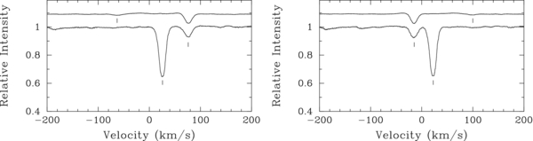
Figure 1. Left: from an AST spectrum of the 1 Gem system, the lower solid line is the average profile of the components, summed from about 170 spectral regions. Tick marks indicate the positions of the Ba (F-subgiant) and A (K-giant) components. The upper line, arbitrarily vertically shifted for visibility, is the remainder after a model of the K-giant component has been removed from the lower line. The position of the extremely weak third component, Bb, is indicated. Right: the same results for another AST spectrum at an orbital phase with the Ba and Bb components reversed.
Download figure:
Standard image High-resolution imageTable 4. 1 Gem Radial-velocity Data Set E (AST)
| HJD−2,400,000.5 | Velocity (A) | σ | O − C | Velocity (Ba) | σ | O − C | Velocity (Bb) | σ | O − C |
|---|---|---|---|---|---|---|---|---|---|
| (km s−1) | (km s−1) | (km s−1) | |||||||
| 52,895.5211 | 20.3 | 0.09 | 0.02 | −15.3 | 0.36 | −0.18 | 103.1 | 2.00 | 0.22 |
| 52,897.5268 | 20.3 | 0.11 | 0.01 | 44.2 | 0.45 | −0.38 | ... | ... | ... |
| 52,898.4772 | 20.3 | 0.09 | 0.00 | 70.2 | 0.36 | −0.16 | −45.0 | 2.00 | −3.64 |
| 52,899.4790 | 20.2 | 0.09 | −0.10 | 81.2 | 0.36 | 0.58 | −56.7 | 2.00 | 1.98 |
| 52,903.4876 | 20.4 | 0.09 | 0.08 | −16.4 | 0.36 | 0.47 | 106.0 | 2.00 | 0.24 |
| 52,904.4837 | 20.3 | 0.09 | −0.03 | −22.3 | 0.36 | 0.42 | 118.0 | 2.00 | 2.37 |
| 52,908.4779 | 20.3 | 0.09 | −0.05 | 77.0 | 0.36 | 0.04 | −52.0 | 2.00 | 0.58 |
| 52,909.4750 | 20.3 | 0.09 | −0.05 | 79.0 | 0.36 | 0.34 | −55.0 | 2.00 | 0.46 |
| 52,910.4751 | 20.4 | 0.11 | 0.04 | 59.6 | 0.45 | −0.24 | ... | ... | ... |
| 52,912.4727 | 20.4 | 0.09 | 0.04 | −2.6 | 0.36 | 0.85 | 88.5 | 2.00 | 5.46 |
Notes. Radial-velocity data for the 1 Gem system from AST, together with the uncertainties and the fit residuals (O − C values) for the fit.
Only a portion of this table is shown here to demonstrate its form and content. A machine-readable version of the full table is available.
Download table as: DataTypeset image
It was noted in the reduction of data set E that some of the lines of the close binary are sufficiently blended with the dominant K-giant's lines that systematic errors could potentially be introduced. We checked this possibility by fitting a model that is limited to only those points in data set E where velocities for all three components are available. The resulting parameters were not significantly different from the fit to all of the data. However, the  of the fit was decreased and the residual velocity scatter was smaller. On the basis of the ratio of residuals we therefore assign separate weights to the two types of data. Points where only the A and Ba components yielded velocities were assigned 25% larger uncertainties than the points when all three were visible.
2.4. Orbital Models
In modeling the hierarchical triple system we make the simplifying assumption that the two orbital systems do not perturb each other, i.e., we use a pair of Keplerian orbital systems, one wide (A–B) and slow (13.3 yr period), the other a close (Ba–Bb) 9.6 day system. Notice that one cannot simply superimpose the separation vectors from the two models; this is because the PHASES observable is the angle between the two centers of light (COL) of the system. Since the A component is single, its center of mass (CM) coincides with its COL. However, for the Ba–Bb system a CM–COL coupling amplitude of the form

is required. Here R = MBb/MBa is the close-orbit mass ratio and L = LBb/LBa the luminosity ratio. Including this coupling term for astrometric data is important when a full analysis including radial-velocity data is made. It is noted that this coupling equation is an approximation valid when rBa-Bb ≪ λ/B and/or L ≪ 1.
To combine optimally the large number of different data sets, taken by different instruments, we group the available radial-velocity data into five separate sets (labeled A through E) and solve for a separate zero-point offset for each data set.
3. RESULTS
The best-fit orbital model was found with the use of an iterative nonlinear least-squares-minimization scheme. The best-fit parameters are given in Table 5. The sigmas (σA through σE) are the standard deviations of the residuals of each set. The astrometric data and best-fit model are provided in Figures 2 and 3. The radial-velocity data and fit are shown Figures 4 and 5. The combined fit to PHASES, radial-velocity, and previous differential astrometry has 1989 data points with 22 free parameters. The reduced  of the fit is 1.16.
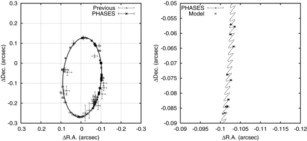
Figure 2. Left: the best-fit visual orbit of the 1 Gem A–Bab system, together with previously available astrometric data and our PHASES astrometry. We note that the error ellipses of the PHASES data appear smaller than the points used to indicate the data. Right: a close-in view of a sub-section of the PHASES astrometry, together with the best-fit orbital model. The predicted locations at the times of measurement are indicated with crosses, but fall underneath the error bars.
Download figure:
Standard image High-resolution image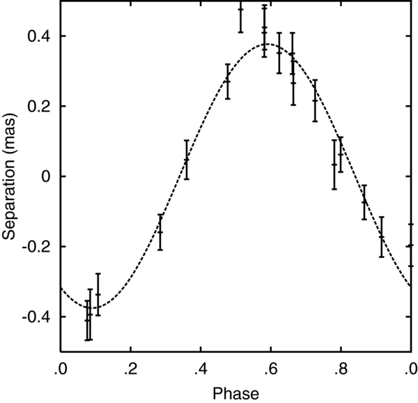
Figure 3. Astrometric orbit of the 1 Gem Bab sub-system projected along an axis rotated 155° east of north. The motion in the A–B system has been removed. The axis corresponds to the most common orientation of the minor axis of the positional error ellipses (which vary slightly from night to night, and between baselines). For clarity, only those observations where the projected uncertainty is less than 300 μ seconds of arc have been included in the plot (all observations are included in the fit).
Download figure:
Standard image High-resolution image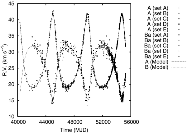
Figure 4. Radial velocities of 1 Gem compared with the computed orbit of the A–B system as a function of time. The motion due to the Ba–Bb orbit has been removed.
Download figure:
Standard image High-resolution image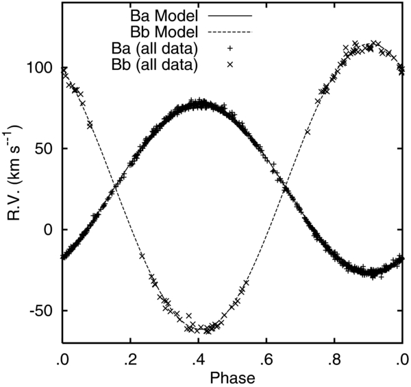
Figure 5. Radial velocities of 1 Gem Ba and Bb compared with the computed orbit. Motion in the A–B system has been removed.
Download figure:
Standard image High-resolution image
Table 5. Best-fit Orbital Parameters for 1 Gem
| Parameter | All Data | Uncertainty | Excluding Set E | Uncertainty | Previous | |||
|---|---|---|---|---|---|---|---|---|
| Value | Value | Value | ||||||
| χ2 | 2390.90 | 933.70 | ||||||
| χr | 1.16 | 1.02 | ||||||
| PAB (days) | 4877.6 | ±1.0 | 4877.7 | ±1.0 | 4821.3a | |||
| eAB | 0.3709 | ±0.0004 | 0.3712 | ±0.0005 | 0.34a | |||
| iAB (deg) | 59.33 | ±0.04 | 59.34 | ±0.05 | 62a | |||
| ωAB (deg) | 21.29 | ±0.09 | 21.3 | ±0.1 | 190a | |||
| TAB (MJD) | 45118.5 | ±2.3 | 45118.5 | ±2.3 | ||||
| ΩAB (deg) | 353.67 | ±0.04 | 353.65 | ±0.04 | 178a | |||
| mA (M☉) | 1.94 | ±0.01 | 1.97 | ±0.03 | ||||
| mB (M☉) | 2.719 | ±0.008 | 2.73 | ±0.02 | ||||
| d (pc) | 46.76 | ±0.07 | 46.9 | ±0.2 | ||||
| PBab (days) | 9.596558 | ±0.000004 | 9.596547 | ±0.000006 | 9.59659 ± 0.00004b | |||
| eBab | 0.0024 | ±0.0005 | 0.005 | ±0.001 | 0.0b | |||
| iBab (deg) | 93.2 | ±1.1 | 95.1 | ±1.3 | ||||
| ωBab (deg) | 164.3 | ±11.8 | 55.1 | ±14.7 | ||||
| T0, Bab (MJD) | 53220.5 | ±0.3 | 53217.6 | ±0.4 | ||||
| T0, Bab (MJD)c | ... | ... | ... | ... | 40443.129 ± 0.015b | |||
| ΩBab (deg) | 137.5 | ±1.9 | 137.5 | ±1.8 | ||||
| mBb/mBa | 0.593 | ±0.001 | 0.599 | ±0.004 | ||||
| LBb/LBa(K-band) | 0.00 | ±0.02 | 0.01 | ±0.02 | ||||
| V0(A, km s−1) | 26.38 | ±0.03 | 26.38 | ±0.03 | ||||
| V0(B, km s−1) | 25.4 | ±0.1 | 25.4 | ±0.1 | ||||
| V0(C, km s−1) | 25.28 | ±0.06 | 25.26 | ±0.06 | ||||
| V0(D, km s−1) | 25.11 | ±0.04 | 25.11 | ±0.04 | ||||
| V0(E, km s−1) | 25.254 | ±0.007 | ... | ... | ||||
| No.Param. | 22 | 21 | ||||||
| No.Pts. | 1989 | 846 | ||||||
| σA (km s−1 | A: 0.65 | Ba: 1.04 | A: 0.65 | Ba: 0.92 | ||||
| σB (km s−1 | A: 0.35 | Ba: 0.89 | A: 0.35 | Ba: 0.96 | ||||
| σC (km s−1 | A: 0.66 | Ba: 1.42 | A: 0.66 | Ba: 1.29 | ||||
| σD (km s−1 | A: 0.30 | Ba: 1.33 | A: 0.30 | Ba: 1.46 | ||||
| σE (km s−1 | A: 0.11 | Ba: 0.50 Bb: 2.07 | ... | ... |
Notes. aFrom Söderhjelm (1999). bFrom Griffin & Radford (1976). cTime of maximum RV.
Download table as: ASCIITypeset image
It might be suggested that the dominance of data set E, to which is attributed 95% of the total weight of the radial-velocity observations although it only covers 49% of the orbital cycle of AB, could warp the solution in undesirable ways. We therefore report the results for two fits in Table 5: one fit including all data sets and a second fit to only the A, B, C, and D data sets. By giving orbital elements that are derived without any input from set E at all, and finding that they are virtually identical to the plenary solution, we demonstrate that there are no perceptible ill effects from the irregular distribution of the data in terms of the phase of the outer orbit. Comparing the solutions, we find that the estimated component masses change by less than 1σ.
The fit to all of the data yields the smallest uncertainties (even when rescaled by the χr of the fit) and the smallest modified Akaike Information Criterion (Akaike 1974; Burnham & Anderson 2002), and therefore we use the results from that fit to derive the system parameters shown in Table 7 below, for the figures, and for the O − C residuals in the data tables.
Note that even with both COL-astrometry and radial-velocity data, there exists a parameter degeneracy corresponding interchanging which is the brighter star; Ω → Ω + 180° and L → Lalt) (Muterspaugh et al. 2006b). However, given the values, we find that the corresponding alternate luminosity ratio is not physically plausible (Lalt = 2.9).
The best-fit value of the K–band luminosity ratio LBb/LBa is not significantly different from zero; as a result, we are not able to place more than a limit on the absolute magnitude of the Bb component.
3.1. Eccentricity of Inner Orbit
A fit to the inner orbit (Bab) with the inner eccentricity as a free parameter results in a slightly non-zero value (eBab = 0.0024 ± 0.0005). Bassett's test (Bassett 1978) yields a T1 statistic (∼20), indicating that the eccentricity of the orbit is statistically significant. In an effort to confirm the reality of the non-zero eccentricity, we performed separate fits to subsets of the data. First, each set of radial velocity data was fit separately to a double Keplerian model. Next, data set E was split into two equal subsets and fit together with the astrometry data. Finally, the PHASES data were split into two subsets and fit together with data set E. Results are shown in Table 6. All of the fits indicate non-zero eccentricity values, with the largest discrepancy being 2σ (between data set A (RV only) and the plenary solution). The fact that all radial-velocity data sets independently indicate a small but non-zero eccentricity is a strong argument against this result being a data artifact or systematic error.
Table 6. Eccentricities by Data Subset
| Data Sets Used | Best-fit eBab Value and Uncertainty |
|---|---|
| A (RV Only) | 0.0055 ± 0.0015 |
| B (RV Only) | 0.0056 ± 0.0063 |
| C (RV Only) | 0.0077 ± 0.0037 |
| D (RV Only) | 0.0105 ± 0.0051 |
| E (RV Only) | 0.0038 ± 0.0006 |
| E subset 1 + all astro | 0.0032 ± 0.0005 |
| E subset 2 + all astro | 0.0030 ± 0.0005 |
| E + PHASES subset 1 | 0.0032 ± 0.0005 |
| E + PHASES subset 2 | 0.0032 ± 0.0005 |
| All data | 0.0024 ± 0.0005 |
Note. Estimated values of eBab for fits to subsets of the data.
Download table as: ASCIITypeset image
3.2. Relative Orbital Inclinations
The mutual inclination Φ of two orbits is given by

where iAB and iBab are the orbital inclinations and ΩAB and ΩBab are the longitudes of the ascending nodes.
The mutual inclination of the orbits in the 1 Gem system is 136.2 ± 1.6 deg (Table 7); it is within the range where Kozai cycles occur (39 2–1408; Kozai 1962), albeit close to a limit. Fabrycky & Tremaine (2007) predicted an increased frequency of systems with mutual inclinations near the limiting values. Our result is consistent with that prediction, as the 1 Gem system has an orbital configuration matching the expected outcome of Kozai Cycle + Tidal Friction (KCTF) evolution (viz., large period ratio, near-circular inner binary, near-critical mutual inclination).
Table 7. Derived System Parameters for 1 Gem
| Parameter | Value and Uncertainty |
|---|---|
| ΦAB-Bab (deg) | 136.2 ± 1.6 |
| π (arcsec) | 0.02139 ± 0.00003 |
| aAB (arcsec) | 0.2010 ± 0.0004 |
| aBab (arcsec) | 0.002638 ± 0.000005 |
| aBab, C.O.L (arcsec) | 0.00097 ± 0.00006 |
| aAB (AU) | 9.399 ± 0.010 |
| aBab (AU) | 0.1234 ± 0.0001 |
| KA(km s−1) | 11.34 ± 0.03 |
| KB(km s−1) | 8.07 ± 0.04 |
| KBa(km s−1) | 52.0 ± 0.1 |
| KBb(km s−1) | 87.7 ± 0.2 |
| mA(M☉) | 1.94 ± 0.01 |
| mBa(M☉) | 1.707 ± 0.005 |
| mBb(M☉) | 1.012 ± 0.003 |
| MK, A(mag) | −0.99 ± 0.06 |
| MK, Ba(mag) | 1.06 ± 0.07 |
Download table as: ASCIITypeset image
3.3. Component Masses and Distance
In Table 7 various derived parameters, including the individual masses, are listed. Those parameters are based on the results from the fit to the complete data set. From our orbital analysis the distance to the 1 Gem system is 46.76 ± 0.07 pc; that compares well to the revised Hipparcos value of 46.9 ± 2.0 (van Leeuwen 2007).
Because of its faint magnitude, the spectral type of Bb cannot be estimated from even our summed spectra. The only estimate that can be given is by comparing its mass to canonical values of spectral type versus mass relations. With a mass of 1.012 M☉ (Table 7) the Bb component corresponds to a G2V star (Cox 1999) (the possibility of Bb being a white dwarf having been excluded by the detection of its spectral lines).
3.4. Component Luminosities
As part of the combined astrometric and radial-velocity fit we can solve for the K-band luminosity ratios of the components. That is because the distance and sub-system total mass are essentially determined by the observations of the wide A–B system, while the sub-system mass ratio is found from the sub-system radial velocities. Therefore, only the component luminosity ratios are dependent on the size of the observed astrometric perturbation.
Because the PTI cannot provide precise determinations of the total system magnitude mK or the A–B system differential magnitude ΔmK, we obtained a Keck adaptive optics image of 1 Gem on MJD 53,227 with a narrowband H2 2–1 filter centered at 2.262 μm. We measured the A–B differential magnitude to be ΔmH2 = 2.043 ± 0.008 at that wavelength. Neugebauer & Leighton (1969) list the K-band magnitude of the 1 Gem system as 2.21 ± 0.06. Using those photometric measurements, together with the parallax and upper limit to the Ba–Bb intensity ratio determined here, we derive the absolute K magnitudes and list them in Table 7.
4. CONCLUSIONS
We have combined PHASES interferometric astrometry with extensive radial-velocity data to measure the orbital parameters of the triple-star system 1 Geminorum, and in particular to resolve the apparent orbital motion of the close Ba–Bb pair. The amplitude of the Ba–Bb COL motion is only 970 ± 60 μas, indicating the level of astrometric precision attainable with interferometric astrometry. The orbital period of the outer A–B pair is 13.354 ± 0.002 yr, while that of the inner Ba–Bb pair is 9.596558 ± 0.000004 days.
By using astrometry and radial velocities to measure both orbits, we are able to determine the mutual inclination of the orbits, which we find to be 1362 ± 16. Such a near-critical mutual inclination is the expected outcome of KCTF evolution (Fabrycky & Tremaine 2007).
We also present the first direct detection of the tertiary component, Bb, in this system. The combination of radial-velocity data for all three components and high-precision astrometry allows us to constrain the mass ratio of the B subsystem, as well as solve for the complete set of system parameters. Finally, we have been able to determine the component masses with precision in the 0.5% range and the distance to the system to 0.15%, among the most precise mass and distance determinations available for stellar multiple systems.
We wish to acknowledge the extraordinary observational efforts of K. Rykoski. He routinely put in extreme amounts of overtime to ensure successful operations and maintenance of an overwhelmingly complex instrument. He developed procedures and operations models that ensured the success of the observatory. The very low amount of lost time due to hardware failures at PTI is a result of his efforts and is unique in the field. Observations with PTI were made possible thanks to the efforts of the PTI Collaboration, which we acknowledge. We also thank the Dominion Astrophysical, Palomar, and Geneva observatories for allowing R.F.G. to obtain radial velocities of 1 Gem. We also thank Lou Boyd, Director of Fairborn Observatory, for dedication to robotic astronomy and excellent maintenance of a unique observatory. This research has made use of services from the Michelson Science Center, California Institute of Technology, http://msc.caltech.edu. Part of the work described in this paper was performed at the Jet Propulsion Laboratory under contract with the National Aeronautics and Space Administration. This research has made use of the Simbad database, operated at CDS, Strasbourg, France, and of data products from the Two-Micron All-Sky Survey, which is a joint project of the University of Massachusetts and the Infrared Processing and Analysis Center/California Institute of Technology, funded by the NASA and the NSF. M.W.M. acknowledges support from State of Tennessee's Centers of Excellence Program and the Townes Postdoctoral Fellowship Program.