


ABSTRACT
We study the mode conversion between different radial orders for solar acoustic waves interacting with sunspots. Solar acoustic waves are modified in the presence of sunspots. The modification in the wave can be viewed as that the sunspot, excited by the incident wave, generates the scattered wave, and the scattered wave is added to the incident wave to form the total wave inside and around the sunspot. The wavefunction of the acoustic wave on the solar surface is computed from the cross-correlation function. The wavefunction of the scattered wave is obtained by subtracting the wavefunction of the incident wave from that of the total wave. We use the incident waves of radial order n = 0–5 to measure the scattered wavefunctions from n to another radial order n' for NOAAs 11084 and 11092. The strength of scattered waves decreases rapidly with |Δn|, where Δn ≡ n' − n. The scattered waves of Δn = ±1 are visible for n ⩽ 1, and significant for n ⩾ 2. For the scattered wave of Δn = ±2, only few cases are visible. None of the scattered waves of Δn = ±3 are visible. The properties of scattered waves for Δn = 0 and Δn ≠ 0 are different. The scattered wave amplitude relative to the incident wave amplitude decreases with n for Δn = 0, while it increases with n for Δn ≠ 0. The scattered wave amplitudes of Δn = 0 are greater for the larger sunspot, while those of Δn ≠ 0 are insensitive to the sunspot size.
Export citation and abstract BibTeX RIS
1. INTRODUCTION
The interaction of solar acoustic waves with magnetic regions modifies the acoustic waves inside and around magnetic regions. The study of interaction is one of major issues in helioseismology because it provides a tool to probe the subsurface structure of magnetic regions. The interaction has been studied by many authors observationally (Thomas et al. 1982; Braun et al. 1987, 1998; Bogdan et al. 1993; Duvall et al. 1993; Braun 1995; Kosovichev 1996; Chen et al. 1996, 1997, 1998; Chang et al. 1997; Chou et al. 1999, 2000, 2009a, 2009b, 2009c; Braun & Lindsey 2000; Kosovichev et al. 2000; Chou 2000; Lindsey & Braun 2000; Zhao et al. 2001; Cameron et al. 2008, 2011; Liang et al. 2010; Zhao et al. 2011, 2011a, 2011b; Yang et al. 2012; Zhao & Chou 2013). It has also been extensively studied theoretically and numerically (Hollweg 1988; Spruit & Bogdan 1992; Chou 1994; Cally et al. 1994; Fan et al. 1995; Chou et al. 1996; Cally & Bogdan 1997; Crouch & Cally 2005; Crouch et al. 2005; Schunker & Cally 2006; Cally & Goosesens 2008; Jain & Gordovskyy 2008; Khomenko et al. 2009; Parchevsky & Kosovichev 2009; Moradi et al. 2010; Hartlep et al. 2011; Jain et al. 2011; Chou et al. 2012; Felipe et al. 2012; Hindman & Jain 2012). A more complete list of references can be found in the review article by Gizon et al. (2010).
The modification in the acoustic wave due to the interaction with magnetic regions can be described by scattered waves. The magnetic region generates a scattered wave as it is perturbed by the incident wave; the scattered wave is added to the incident wave to form the total wave in and around the magnetic region. Zhao et al. (2011a) have measured the wavefunctions of scattered waves from a radial order to the same radial order. In this study, we measure the wavefunctions of scattered waves between different radial orders.
2. SCATTERED WAVES
In the absence of magnetic field, the wavefunction of the solar acoustic wave, Ψ0, satisfies a homogeneous wave equation  , where
  is a linear wave operator, depending on the properties of the quiet Sun. If a magnetic region is present,
  would be modified to
  , where
  describes the perturbation in the magnetic region. The wavefunction Ψ0 is modified to Ψ, and Ψs ≡ Ψ − Ψ0 is called the scattered wave. The wave equation becomes
  , or it can be expressed as an inhomogeneous wave equation
  , where
  is a source term, describing the interaction between the incident wave and the magnetic region. Here we use the scattered wavefunction Ψs to study the scattering of acoustic waves by a magnetic region, like the scattering problems in other physics disciplines, for example, electrodynamics (Jackson 1999), quantum mechanics (Schiff 1968), and mathematical physics (Morse & Feshbach 1953). The scattered wavefunction Ψs can be solved as
  , where
  is the Green's function satisfying
  , and where δ(x) is the Dirac delta function. Since the scattered wavefunction Ψs directly relates to the source S, the measured Ψs provides information on the interaction with the magnetic region.
The scattered wavefunction Ψs can be understood as follows. The incident wave Ψ0 propagates from the quiet Sun toward a sunspot (magnetic region) and interacts with it. The interaction generates the signal Ψs inside the sunspot; Ψs propagates away from the sunspot and is added to Ψ0 to form the total wave Ψ inside and around the sunspot. The scattered wave depends on the incident wave. The simplest incident wave is a plane wave in the horizontal direction (x, y), which is the eigenfunction in the planar atmosphere of the quiet Sun. The plane wave is characterized by the mode parameters (n, kx, ky), where n is the radial order, and kx and ky are the x and y components of the horizontal wavenumber vector  , respectively. From the dispersion relation in the solar rotating reference frame, each (n, kx, ky) is associated with a frequency ω, which is a function of n and
  .
.
If the sunspot is stable, the scattering is time-independent. The frequency of the scattered wave is the same as that of the incident wave. The interaction could convert the incident p mode (n, kx, ky) into other p modes  , while keeping the frequency ω unchanged. The two sunspots in this study were rather stable during the period of study. Thus, the time-independent scattering is a reasonable approximation for our case.
The interaction with sunspots could also convert the incident p mode into modes other than p modes, such as magnetoacoustic modes and jacket modes (Bogdan & Cally 1995). In helioseismology, the mode conversion among p modes is usually called the mode mixing (D'Silva 1994; Braun 1995), and the term "mode conversion" is used for the conversion from p modes to magnetoacoustic modes (Cally & Bogdan 1993; Hindman & Jain 2012). Here, we use the term "mode conversion" in a general sense, and specify the type of conversion to make distinctions.
If n' = n, the incident mode and the scattered modes are on the same ridge in the k − ω diagram, and k' = k because ω remains the same, but the directions of  and
and  could be either the same or different. The incident mode could also be converted into other radial orders; that is, the mode on ridge n could be converted to the modes on another ridge n'. Since ω has to remain unchanged, for this case, k' ≠ k and the directions of
  and
and  could be either the same or different. The value of k' depends on k, n, and n' through the relation ω(n, k) = ω(n', k'). Zhao et al. (2011a) have measured the scattered wavefunctions for the case of n' = n with n = 0–5. In this study, we measure the scattered wavefunctions for n' ≠ n.
3. DATA AND PRELIMINARY REDUCTION
The data and preliminary data reduction is identical to that in Zhao et al. (2011a). Here we give only a brief description. The helioseismic data in this study are taken with Helioseismic and Magnetic Imager on board the Solar Dynamical Observatory (Scherrer et al. 2012; Schou et al. 2012). The data are 4096 × 4096 full-disk Dopplergrams taken at a rate of one image every 45 s. Two active region NOAAs, 11084 and 11092, are studied: a time series of 12,402 frames is used for NOAA 11084 and 13,616 frames for NOAA 11092. The time series is divided into 2048 frame sets. Each set is analyzed separately, and the results are averaged over different sets. The following analysis is carried out for each set.
The preliminary data reduction procedure is similar to that in Chou et al. (2009a) and Zhao et al. (2011a), and is briefly described as follows. (1) The slow temporal variations in the data are removed by subtracting the 81 frame running mean from the signal at each spatial point. (2) The radial component of the Doppler signal is restored from the measured line-of-sight component with a geometrical correction. (3) The signals below 1.5 mHz are removed with a high-pass temporal filter; the edge of the filter is smoothed with a half cosine-bell function (Hann window) in the range of 1.5–2 mHz. (4) Each full-disk image is transformed into coordinates of longitude and latitude, and the differential rotation of the solar surface is removed. (5) A selected area is transformed into a coordinate system of (ϕ, θ) centered at the sunspot center, where ϕ is the east-west direction and θ the north-south direction. The dimension of the selected region is 60° in ϕ and 60° in θ, corresponding to 1024 × 1024 pixels (0 0586 or 0.712 Mm per pixel). For convenience, we use the coordinate system (x, y) to represent (ϕ, θ) in the following discussion.
After the above preliminary analysis, the data cube of (x, y, t) is ready for the computations in Section 4. The magnetic and acoustic-power maps of the selected area are shown in Figure 1. The radius of penumbra is about 088 (15 pixels) for NOAA 11084 and 117 (20 pixels) for NOAA 11092. That the region around the sunspot is relatively quiet makes these two regions ideal for this study.

Figure 1. Magnetic and acoustic-power maps of NOAA 11084 (upper panels) and NOAA 11092 (lower panels; from Zhao et al. 2011a). The dimension of each map is 60° × 60° (1024 × 1024 pixels). The magnetic maps are in units of Gauss. The acoustic power is set to unity in the quiet Sun. The radius of the penumbra is 15 pixels for NOAA 11084 and 20 pixels for NOAA 11092.
Download figure:
Standard image High-resolution image4. MEASUREMENTS OF SCATTERED WAVEFUNCTIONS
The discussion in Sections 4.1 and 4.2 is similar to that in Zhao et al. (2011a).
4.1. Incident Waves
As discussed in Section 2, the simplest incident wave for our scattering problem is the eigenfunction (single mode) of the quiet Sun. However, the scattered wave associated with a single-mode incident wave is too weak to be detected. Here, we use a wave packet, formed by the modes with a particular n, propagating in a particular horizontal direction as the incident wave like Cameron et al. (2008) and Zhao et al. (2011a). First, the waves of a particular n are isolated by filtering the modes on the ridge of n in the Fourier domain (kx, ky, ω). These waves propagate horizontally in all directions. To obtain the incident wave propagating in a particular horizontal direction, the signals on a line, called the reference line, perpendicular to the propagation direction are averaged. The reference line is located outside the sunspot and parallel to the x axis at y = y0; that is, the incident wave propagates in the y direction. The line-averaged signal is denoted by  . This incident wave is a wave packet formed by superposing modes (n, kx = 0, ky), where n is fixed. In this study, the reference line is 70 pixels (41 or 50 Mm) from the sunspot center.
4.2. Measurements of Wavefunctions
The propagation of the incident wave can be studied by computing the cross-correlation function (CCF) between the line signal  and the signal at (x, y), Ψ(x, y, t),
where * denotes the complex conjugate, and the constant A is selected such that  in Equation (2) is unity at y = y0 and τ = 0. The CCF C(x, y, τ) picks up the signals within Ψ(x, y, t) that correlate with the line signal
  at a time shift τ. Although C(x, y, τ) describes the propagation of the wave packet starting from the reference line, it is not the wavefunction. The wavefunction associated with C(x, y, τ) can be computed as (Zhao et al. 2011a)
where C(x, y, ω) is the Fourier component of C(x, y, τ), Ψ(x, y, ω) and  are the Fourier components of Ψ(x, y, t) and
  , respectively, and
  (x, y, ω) and
  are the phases of Ψ(x, y, ω) and
  , respectively. The wavefunction
  is not identical to the wavefunction Ψ(x, y, τ), which is formed by the modes with random phases (x, y, ω). For each Fourier component,
  has an amplitude equal to that of Ψ(x, y, ω), but with a phase relative to that of the line signal,
  . Thus,
  represents an organized wave packet starting from the reference line at time zero and arriving at (x, y) at time τ. This organized wave packet, instead of Ψ(x, y, τ), is what we would like to measure.
The signals computed in Equation (2) are weak relative to noise. Two averagings are carried out to enhance the signal-to-noise ratio (Zhao et al. 2011a). The first one is the average over different propagation directions. For each direction, the reference line is at the same distance from the sunspot center. A total of 3000 different directions are used, corresponding to a step of 012. The mapping of data into (θ, ϕ) coordinates in Section 3 is repeated for each orientation such that the incident wave always propagates in the θ (or y) direction. The wavefunctions  of 3000 orientations are averaged. The second averaging is over 15 consecutive 2048 frame data sets for NOAA 11084 and 17 consecutive data sets for NOAA 11092.
4.3. Scattered Wavefunctions of the Same Radial Order
If both the line signal  and the point signal Ψ(x, y, t) in Equation (1) are filtered with the same ridge filter of n, the wavefunction
  represents the wave packet of n propagating from the reference line at time zero to the location (x, y) at time τ. This is the case studied in Zhao et al. (2011a). The wave packet would be modified as it propagates through the sunspot. Behind the sunspot,
  is the sum of the incident wave and scattered wave. To obtain the scattered wavefunction, we need to subtract the wavefunction of the incident wave from
  . The incident wavefunction can be computed from the quiet Sun. The above procedure is carried out for 25 quiet regions to obtain the wavefunction without being affected by the sunspot, denoted as
  , which is used as the wavefunction of the incident wave. The difference,

is the wavefunction of the scattered wave. Since the line signal could propagate in both ±y directions, to obtain the scattered wavefunction propagating in the y direction, we apply a direction filter to isolate  propagating in the y direction. The results of
  for n = 0–5 have been measured and discussed in Zhao et al. (2011a). An improvement on the direction filter is made here to reduce the residuals of
  around τ = 0, shown in Figures 3(a) and 4(a) in Zhao et al. (2011a). In Zhao et al. (2011a), the direction filter is applied to a range of −30 ⩽ y ⩽ 540 pixels, while the direction filter here is applied to a range of −400 ⩽ y ⩽ 540 pixels, where the reference line is at y = 0. The residuals of
  around τ = 0 in this study are much weaker than those in Zhao et al. (2011a).
4.4. Scattered Wavefunctions of Different Radial Orders
If the line signal  in Equation (1) is filtered with a ridge filter of n while the point signal Ψ(x, y, t) is filtered with another ridge filter of n',
  would be the signal of n' that correlates with the incident line signal of n; that is,
  is the signal that is converted from the incident signal of n to n' by the interaction with the sunspot. Since there is no signal converted from n to n' in the quiet Sun,
  measured in the quiet regions contains no signal, simply fluctuating noise. Thus,
  . For convenience, the scattered wavefunction from n to n' is denoted as
  and Δn ≡ n' − n.
In this study, we measure scattered wavefunctions  for n = 0–5 and n' = 0–5. The strength of scattered waves decreases rapidly with |Δn|. The scattered waves of Δn = ±1 are visible for all ns. For Δn = ±2, only few cases are visible. None of Δn = ±3 are visible. Figures 2 and 3 show the scattered wavefunctions of Δn = 0, 1, and 2 for n = 0. Figures 4 to 11 show the scattered wavefunctions of Δn = 0 and ±1 for n = 1–4. Figures 12 and 13 show the scattered waves of Δn = 0, −1, and −2 for n = 5. Figure 14 shows the scattered waves of Δn = ±2 for n = 3, NOAA 11084. It is noted that the gray scales of Figures 6–13 are identical, but those of Figures 2–5 and 14 are different. The animations associated with Figures 8 and 14 are provided as examples. In the animations, the interval between successive frames is 45 s; the clock at the upper right corner is the actual lapse of time. It should be mentioned that Braun (1995) has reported the evidence of mode conversion between adjacent radial orders from the correlation of the phases of ingoing p modes with the phases of outgoing p modes in the Hankel analysis.

Figure 2. Spatial distribution of scattered wavefunctions  (left column),
  (central column), and
  (right column) of NOAA 11084 at three different times. The dimension of each panel is 400 × 400 pixels (00586 or 0.712 Mm pixel−1). Some signal of
  is barely visible inside the sunspot, but lost in the background fluctuation once it propagates out of the sunspot. The scattered wave
  is not visible.
Download figure:
Standard image High-resolution image
Figure 3. Same as Figure 2, but for NOAA 11092.
Download figure:
Standard image High-resolution image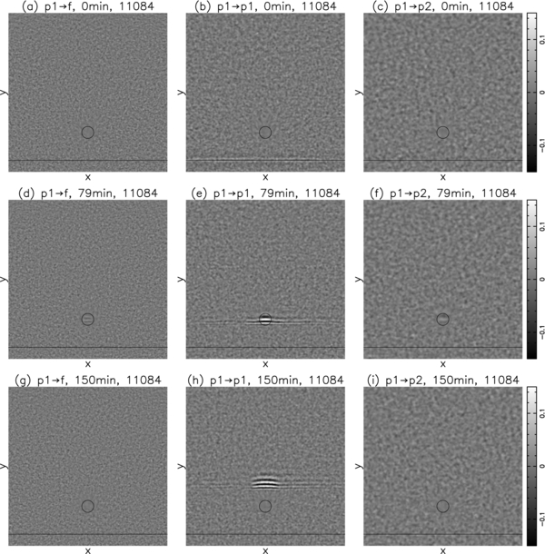
Figure 4. Spatial distribution of scattered wavefunctions  (left column),
  (central column), and
  (right column) of NOAA 11084 at three different times. The dimension of each panel is 400 × 400 pixels (00586 or 0.712 Mm pixel−1). The signals of
  and
and  are visible inside and behind the sunspot, but soon lost in the background fluctuation outside the sunspot.
Download figure:
Standard image High-resolution image
Figure 5. Same as Figure 4, but for NOAA 11092.
Download figure:
Standard image High-resolution image
Figure 6. Spatial distribution of scattered wavefunctions  (left column),
  (central column), and
  (right column) of NOAA 11084 at three different times. The dimension of each panel is 400 × 400 pixels (00586 or 0.712 Mm pixel−1).
Download figure:
Standard image High-resolution image5. PROPERTIES OF SCATTERED WAVES
Here we discuss the properties of these measured scattered wavefunctions. One apparent phenomenon in Figures 2–13 is that the amplitude of scattered wave of Δn = 0 is greater than those of Δn ≠ 0 for all ns under study. The amplitude difference between Δn = 0 and Δn = ±1 is greatest for n = 0 and decreases with n. For n = 5, the amplitude of the scattered wave of  is comparable to that of
  .
.
The amplitude of scattered waves shown in Figures 2–13 increases with n for both Δn = 0 and Δn ≠ 0. The shorter lifetime (greater dissipation) of smaller n may in part account for this phenomenon. Thus, the amplitude of the scattered wave should be compared with that of incident wave. Zhao et al. (2011a) plotted the incident wave amplitude and the scattered wave amplitude of Δn = 0 together for comparison (Figure 8 therein), and found that the ratio of scattered wave amplitude to incident wave amplitude decreases with n, although the apparent scattered wave amplitude increases with n. For the same purpose, Figures 15 and 16 show the comparison of the wave amplitudes of incident and scattered waves versus y for Δn = −1 and Δn = 1, respectively. In contrast to Δn = 0, these two figures indicate that, for Δn ± 1, the ratio of scattered wave amplitude to incident wave amplitude increases with n. It is worth pointing out that this observational result is opposite to the result of a theoretical study by Hindman & Jain (2012). They have studied the scattering of acoustic waves by a vertical thin magnetic flux tube, and found that the fraction of energy conversion between different radial orders decreases with n.
For n = 0 (Figures 2 and 3), the scattered wave  is barely visible inside the sunspot, but lost in the background fluctuations once it propagates out of the sunspot. The scattered wave
  is not visible. It should be mentioned that the simulation study of Felipe et al. (2012) suggests that a small amount of power of f modes is scattered into p1 modes in their magnetic flux tube models. For n = 1 (Figures 4 and 5), the scattered waves of Δn ± 1 are visible inside and behind the sunspot, but are soon lost in the background fluctuations outside the sunspot. For n = 2 (Figures 6 and 7), the scattered wave amplitude of Δn = 1 is greater than that of Δn = −1. For n = 3 and 4 (Figures 8 to 11), the situation is opposite: The scattered wave amplitude of Δn = −1 is greater than that of Δn = 1. It is noted that in the theoretical study of Hindman & Jain (2012), the fraction of energy conversion of Δn < 0 is always greater than that of Δn > 0 for all ns.
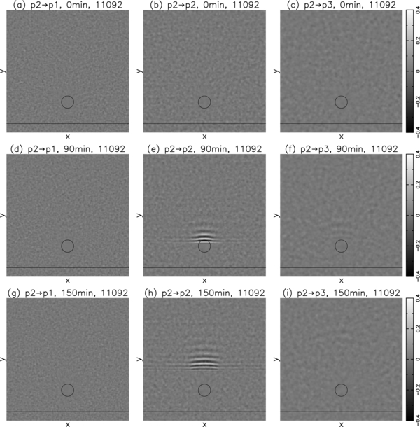
Figure 7. Same as Figure 6, but for NOAA 11092.
Download figure:
Standard image High-resolution image
Figure 8. Spatial distribution of scattered wavefunctions  (left column),
  (central column), and
  (right column) of NOAA 11084 at three different times. The dimension of each panel is 400 × 400 pixels (00586 or 0.712 Mm pixel−1).(An animation of this figure is available in the online journal.)
Download figure:
Standard image High-resolution imageAnother interesting phenomenon is the relative scattered wave amplitudes of NOAAs 11084 and 11092. The sunspot size ratio of NOAA 11092 to 11084 is 4/3. For Δn = 0, the scattered wave amplitude of NOAA 11092 is clearly greater than that of NOAA 11084 for all ns. However, for Δn = ±1, the scattered waves of NOAAs 11084 and 11092 are comparable. For some cases, the scatter wave amplitude of NOAA 11084 is even greater than that of NOAA 11092, for example,  and
and  . This can be seen in Figures 6 to 9, 15, and 16.

Figure 9. Same as Figure 8, but for NOAA 11092.
Download figure:
Standard image High-resolution image
Figure 10. Spatial distribution of scattered wavefunctions  (left column),
  (central column), and
  (right column) of NOAA 11084 at three different times. The dimension of each panel is 400 × 400 pixels (00586 or 0.712 Mm pixel−1).
Download figure:
Standard image High-resolution image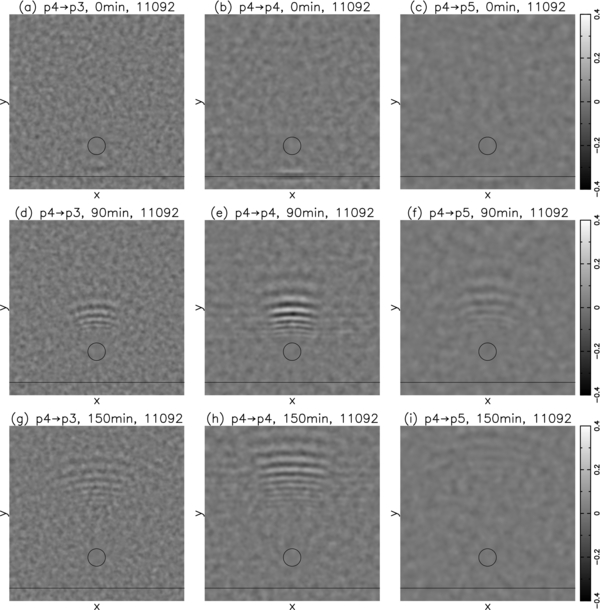
Figure 11. Same as Figure 10, but for NOAA 11092.
Download figure:
Standard image High-resolution imageThe scattered waves of Δn ± 2 are shown in Figures 12 to 14. In Figure 12,  of NOAA 11084 is barely seen in the middle row. In Figure 13,
  of NOAA 11092 is less visible. In Figure 14,
  and
and  of NOAA 11084 are barely seen. The animation associated with Figure 14 is provided. The corresponding scattered waves for NOAA 11092 are not shown here because they are less visible.
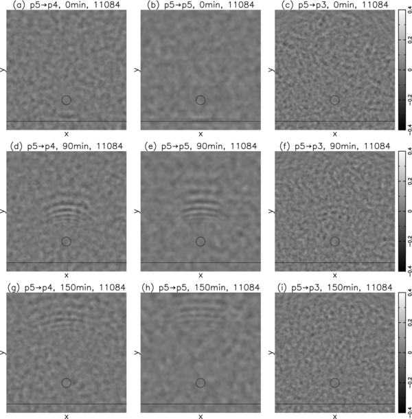
Figure 12. Spatial distribution of scattered wavefunctions  (left column),
  (central column), and
  (right column) of NOAA 11084 at three different times. The dimension of each panel is 400 × 400 pixels (00586 or 0.712 Mm pixel−1). The strengths of
  (left column) and
  (central column) are comparable. The scattered wave
  (right column) is barely seen at τ = 90 minutes.
Download figure:
Standard image High-resolution image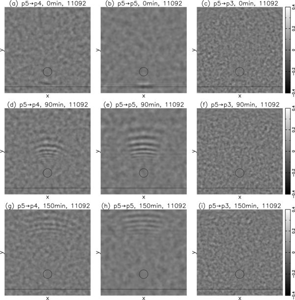
Figure 13. Same as Figure 12, but for NOAA 11092.
Download figure:
Standard image High-resolution image
Figure 14. Spatial distribution of scattered wavefunctions  (left column),
  (central column), and
  (right column) of NOAA 11084 at three different times. The dimension of each panel is 400 × 400 pixels (00586 or 0.712 Mm pixel−1). The scattered waves
  (left column) and
  (right column) are barely seen at τ = 43 and 77 minutes. Note that the gray scale is different from that in Figure 8.(An animation of this figure is available in the online journal.)
Download figure:
Standard image High-resolution image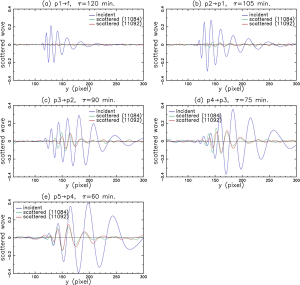
Figure 15. Comparison of the scattered wave amplitude of Δn = −1 with the incident wave vs. y for n = 1–5. The wave amplitude is averaged over 30 pixels in the x direction, centered at the sunspot center. The sunspot is centered at y = 100. The radius of the penumbra is 15 pixels for NOAA 11084 and 20 pixels for NOAA 11092. Each pixel is 00586 (or 0.712 Mm).
Download figure:
Standard image High-resolution image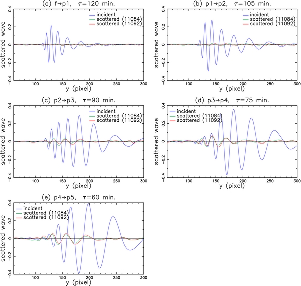
Figure 16. Same as Figure 15, but for Δn = 1, n = 0–4.
Download figure:
Standard image High-resolution image
6. DISCUSSION
The scattered wave, defined as the subtraction of the incident wave from the total wave, consists of all effects of the interaction with magnetic regions, including the phase shift, absorption (decrease in wave energy), elastic scattering, and the conversion into waves other than p-mode waves. All these effects are manifested by the interference between the incident wave and the scattered wave. For example, a decrease in wave amplitude could in part be due to the destructive interference between the scattered wave and the incident wave. From the definition, the scattered wave includes p modes as well as magnetoacoustic modes in the magnetic regions. However, since the ridge filters are applied to the data before computing the CCF, the measured scattered wavefunction in this study contains only p modes, and does not include magnetoacoustic modes even inside the magnetic regions.
In terms of energy removal from the incident wave, the interaction is in general divided into two different mechanisms, absorption (inelastic scattering) and elastic scattering (Schiff 1968; Jackson 1999). In helioseismology, the conversion from one p mode into other p modes is the elastic scattering. The concept of absorption in helioseismic measurements is more complicated. It has been observed, for example, with Hankel analysis (Braun et al. 1987), that the p-mode energy decreases as p modes pass through sunspots. Several mechanisms have been proposed to explain this observed energy decrease. The most popular one is that an incident p mode is converted into magnetoacoustic modes, which could dissipate into heat in a thin resonance layer (Hollweg 1988) or propagate along the magnetic field out of the p-mode cavity (Cally & Bogdan 1993; Crouch & Cally 2005; Gordovskyy & Jain 2008). Another possible contribution, which has nothing to do with absorption, to this observed energy decrease is the emissivity reduction in magnetic regions (Parchevsky & Kosovichev 2007; Chou et al. 2009a, 2009b). It is noted that the emissivity reduction does not enter our measured wavefunctions because they are obtained from the CCFs.
For the cases of Δn = 0, both absorption and elastic scattering are present. A part of the incident the p mode is converted into other p modes with the same k and ω, but propagating in different directions. This part is the elastic scattering. The fact that the total energy of all scattered waves is less than the total energy of the incident wave indicates the presence of absorption. For the cases of Δn ≠ 0, the incident wave of n is converted into the scattered wave of n'; apparently only the elastic scattering is involved.
The phenomenon regarding the sunspot size discussed in the fourth paragraph of Section 5 suggests that absorption is greater for the larger sunspot, while the elastic scattering is less sensitive to the sunspot size. Another phenomenon discussed in the second paragraph of Section 5 is that the scattered wave amplitude relative to the incident wave amplitude decreases with n for Δn = 0, while increases with n for Δn ≠ 0. This suggests that the absorption cross section decreases with n, while the elastic scattering cross section increases with n.
For a detailed study of the scattering problem and its interaction, a common tool is the scattering matrix (S-matrix). Let {φβ} be a complete set of orthonormal eigenfunctions of the quiet Sun, where β denotes the mode parameters (n, kx, ky). For a given incident wave φα, the associated scattered wave, denoted by  , can be expanded in terms of {φβ}:
  . The expansion coefficients Tβα are called the T-matrix elements of scattering. The S-matrix is the sum of the unit matrix and the T-matrix. The S-matrix elements provide the most complete observational information on the interaction. Our ultimate goal is to obtain the S-matrix elements from the measured scattered wavefunctions presented in this study.
7. SUMMARY
Using the method developed by Zhao et al. (2011a), we measure the scattered wavefunction from a radial order n to another radial order n' for n = 0–5 for NOAAs 11084 and 11092. The strength of scattered waves decreases rapidly with |Δn|. The scattered waves of Δn = ±1 are visible for n ⩽ 1, and significant for n ⩾ 2. For the scattered wave of Δn = ±2, only few cases are visible. None of the scattered waves of Δn = ±3 are visible. The properties of scattered waves for Δn = 0 and Δn ≠ 0 are different. For Δn = 0, the ratio of scattered wave amplitude to incident wave amplitude decreases with n, while it increases with n for Δn ≠ 0. The scattered wave of Δn = 0 is stronger for the larger sunspot for all ns, while the scattered wave amplitudes of two sunspots are comparable for Δn ≠ 0. For some cases, the scattered wave of the smaller sunspot is even stronger.
The SDO/HMI data are provided by the HMI team at Stanford University. H.Z. is supported by the NSF of PRC under grants 112201063 and 11303053. D.Y.C. is supported by the NSC of ROC under grant NSC-102-2112-M-007-022-MY3.