


ABSTRACT
We present global coronal seismology for the first time, which allows us to determine inhomogeneous magnetic field strength in the extended corona. From the measurements of the propagation speed of a fast magnetosonic wave associated with a coronal mass ejection (CME) and the coronal background density distribution derived from the polarized radiances observed by the STEREO SECCHI COR1, we determined the magnetic field strengths along the trajectories of the wave at different heliocentric distances. We found that the results have an uncertainty less than 40%, and are consistent with values determined with a potential field model and reported in previous works. The characteristics of the coronal medium we found are that (1) the density, magnetic field strength, and plasma β are lower in the coronal hole region than in streamers; (2) the magnetic field strength decreases slowly with height but the electron density decreases rapidly so that the local fast magnetosonic speed increases while plasma β falls off with height; and (3) the variations of the local fast magnetosonic speed and plasma β are dominated by variations in the electron density rather than the magnetic field strength. These results imply that Moreton and EIT waves are downward-reflected fast magnetosonic waves from the upper solar corona, rather than freely propagating fast magnetosonic waves in a certain atmospheric layer. In addition, the azimuthal components of CMEs and the driven waves may play an important role in various manifestations of shocks, such as type II radio bursts and solar energetic particle events.
Export citation and abstract BibTeX RIS
1. INTRODUCTION
Waves in the solar atmosphere have been observed and studied in detail for several decades as they are thought to play an important role in coronal heating and solar wind acceleration (see the reviews by Ofman 2005, 2010, and others). Another important application of waves is coronal seismology (Uchida 1970; Roberts et al. 1984; Aschwanden et al. 1999; Nakariakov et al. 1999; Nakariakov & Ofman 2001; Nakariakov & Verwichte 2005; Ballai 2007; Chen et al. 2011; West et al. 2011), a discipline that studies oscillations in the corona to derive basic physical quantities of the coronal medium, such as magnetic field, density, and temperature from measured and theoretically known wave properties. For the most part, magnetic field strengths remain unknown quantities in the extended solar corona, yet are the most basic parameters in understanding almost all kinds of solar coronal activity.
The physical parameters determined from coronal seismology can be directly applied to interpretations of manifestations of coronal waves and/or shocks accompanied by flares and coronal mass ejections (CMEs). To date, the interpretations of the observations have been performed based on modeled physical parameters (Uchida 1968; Mann et al. 1999, 2003; Gopalswamy et al. 2001; Warmuth & Mann 2005; Evans et al. 2008; Yang & Chen 2010). For instance, Moreton waves observed as chromospheric disturbances associated with flares were interpreted as shocks in the chromosphere due to refracted fast magnetosonic waves traveling in the corona, with a spherically symmetric modeled corona (Uchida 1968). EIT waves have been thought to be the coronal counterparts of Moreton waves (Thompson et al. 1999), but Yang & Chen (2010) showed that the speeds of EIT waves have significant negative correlations with the magnetic field strengths determined with a potential field model, indicating that EIT waves are not fast magnetosonic waves (cf. Warmuth & Mann 2005). Gopalswamy et al. (2001) determined radial profiles of fast magnetosonic speeds above the active region and quiet Sun, using modeled profiles of electron density (Saito et al. 1977) and magnetic field strength (Dulk & McLean 1978; Mann et al. 1999). They argued that shocks may be formed when CME's ejecta cross over a region, azimuthally, where the local fast magnetosonic speed decreases steeply, that is, from active region corona to quiet Sun corona. Along the same line, Evans et al. (2008 and references therein) investigated Alfvén speed profiles derived from MHD models in order to find the origin of multiple shocks driven by a single source (Cho et al. 2011; Feng et al. 2013). In addition, Kahler & Reames (2003) proposed that the angular width of CMEs may play an important role in the formation of shocks and the subsequent gradual solar energetic particles (SEP) events by interactions between azimuthally expanding CMEs and the highly inhomogeneous coronal medium.
These works suggest that physical parameters should be measured by observations, covering very wide spatial range of the solar corona. However, to date, coronal seismology has been applied to localized magnetic structures (e.g., coronal loops or streamers; Aschwanden et al. 1999; Nakariakov et al. 1999; Nakariakov & Ofman 2001; Ofman & Wang 2008; Chen et al. 2011), a specific coronal layer (e.g., EIT waves; Ballai 2007; West et al. 2011), and the radial or near radial direction (e.g., type II radio bursts and shocks ahead of CME leading edges; Vršnak et al. 2002; Mancuso et al. 2003; Cho et al. 2007; Gopalswamy & Yashiro 2011; Gopalswamy et al. 2012; Kim et al. 2012; Poomvises et al. 2012). Alternatively potential field source surface (PFSS) models (Schatten et al. 1969; Altschuler & Newkirk 1969) can be used to find the global coronal magnetic field through extrapolation. However, again, these models cannot take density structures into account (Gary 2001) while, evidently, most coronal phenomena are combination of the magnetic field and plasma. To our knowledge, no coronal seismology has been applied to determine the physical parameters covering a wide azimuthal range of the extended solar corona.
Recently, Kwon et al. (2013, hereafter Paper I) showed a disturbance propagating globally in the extended solar corona, associated with an EIT wave in the low solar corona, using the COR1 inner coronagraphs (Thompson et al. 2003) of the Sun Earth Connection Coronal and Heliospheric Investigation (SECCHI; Howard et al. 2008) instruments on board the twin Solar TErrestrial RElations Observatory (STEREO; Kaiser et al. 2008) spacecraft. The disturbance was observed as a radial density enhancement in the field-of-view of the COR1 coronagraphs (1.5–4.0 R☉) and traveled in a wide azimuthal range, more than 200° of heliocentric angle, passing through coronal streamers that are thought to be the global magnetic separatrices. They derived a radial profile of magnetic field strength from the average speeds and electron densities and found that the profile is consistent with values expected from theoretical and empirical models (Mann et al. 1999; Dulk & McLean 1978), indicating that the speeds of the disturbance are in fact the local fast magnetosonic speeds. With these pieces of observational evidence, they concluded that the propagating disturbance is a true fast magnetosonic wave in association with a CME. Note that their conclusion implies that fast magnetosonic waves observed by the COR1 inner coronagraphs can be used to determine the inhomogeneous magnetic field strength in the azimuthal direction in the heliocentric distance range of 1.5–4.0 R☉. As a matter of fact, the existence of fast magnetosonic waves in the extended solar corona was previously expected by observations of deflections of coronal streamers (e.g., Sheeley et al. 2000), but the propagating wave fronts were undetectable because of the poor time cadence of coronagraphs such as SOHO LASCO C2/C3. Note that the time cadence of the COR1 coronagraphs is five minutes so that the wave fronts and their kinematics became observable and directly measurable.
This paper presents the first application of the new finding, which is global coronal seismology, and the verification of our knowledge of coronal medium and waves/shocks with determined physical quantities, while Paper I presented evidence of the finding. Note that a front should be well established as a true wave front before the application of coronal seismology, but it is a non-trivial problem as we can see from the long-standing debate on the EIT wave (Asai et al. 2012; Chen & Wu 2011; Ma et al. 2011; Olmedo et al. 2012 and references therein). In order to meet this basic requirement and avoid the misuse of the method, we use the disturbance that has been well established as a true fast magnetosonic wave in Paper I. In Section 2, we present the methods of determining electron densities and magnetic field strengths using data set taken from the STEREO SECCHI COR1 inner coronagraphs. In Section 3, we show determined physical parameters, such as electron density, magnetic field strength, and plasma β parameter. In Section 4, we show errors in measuring magnetic field strength, comparisons with previous results, and the physical implications for interpretations of waves/shocks. Finally, brief conclusions are given in Section 5.
2. DATA AND METHODS
We used a data set taken on 2011 August 4 by the STEREO SECCHI COR1 inner coronagraphs (Thompson et al. 2003). STEREO consists of twin spacecrafts and they provide simultaneous observations of the solar corona from nearly opposite directions with a separation angle of ∼167° at that time. The COR1 coronagraphs provide the observations of the extended solar corona in a heliocentric distance range about 1.5–4.0 R☉. The resolution of the COR1 images is 15 arcsec pixel−1 and each image consists of 512 by 512 pixels. The time cadence of the polarized brightness (pB) images or the total brightness images is five minutes.
Paper I showed a relation between the magnetic field strength and the fast magnetosonic speed (vf) in a homogeneous medium in the linear approximation, supposing a simple case that the wave front propagates perpendicular to the magnetic field lines,
where B, ρ, vf, and cs are magnetic field strength, mass density, speed of the fast magnetosonic wave, and sound speed (in cgs units), respectively. The sound speed is set to a constant with assumptions of the fully ionized ideal gas with a temperature T = (1.5 ± 0.5) × 106 K (e.g., Withbroe 1988) and an adiabatic index γ = 1 (Van Doorsselaere et al. 2011). These values give cs = 155 ± 27 km s−1.
The low solar corona below ∼5 R☉ is dominated by the K coronal component which arises from Thomson scattering of the photospheric light from the free electrons and the determination of the electron density at this height range can be done by inverting the pB images (e.g., Billings 1966; Hayes et al. 2001). The observed pB signal can be expressed as an integration of electron density ne(s) along a line of sight (LOS) in the optically thin medium, that is
where ξ is the perpendicular distance between the LOS and the solar center, r is the radial distance from the solar center in the three-dimensional (3D) space, s is measured along the LOS, B☉ is the mean solar brightness, σ = 6.65 × 10⁻²⁵ cm2 is the Thomson scattering cross-section, and u is the limb darkening coefficient. In this study, we took u = 0.6 for the wavelength of the COR1. In addition, A(r) and B(r) are geometrical factors (see Billings 1966; Kramar et al. 2009 for detailed descriptions of pB inversion).
To calculate the distribution of electrons in the corona from the pB images with Equation (2), the simplest way is to assume the density following the spherical symmetric distribution (Spherical Symmetric Inversion, hereafter the SSI method). This method has been applied in many studies (e.g., Saito et al. 1977; Hayes et al. 2001; Quémerais & Lamy 2002). In this study, we assumed that the electron density along a radial trace can be expressed in a polynomial expansion form, i.e., ne(r) =  . Then the coefficients ak can be determined by a least-squares fit to the pB profile along a certain azimuthal position on the solar image. Note that the spherical symmetry is assumed to hold only locally. Therefore, applying this pB inversion to all azimuthal positions, we obtained the density distribution over the entire corona in the plane of the sky (POS). In practice, we used 11 pB images taken from 03:00 to 03:50 UT 2011 August 4 and took the average over the time for this inversion.
The tomography technique has been developed to a more advanced method, which reconstructs 3D coronal density structures by using observations from multiple viewing directions. This technique was previously studied (Davila 1994; Zidowitz 1999) and has been applied to the SOHO LASCO C2 (Frazin et al. 2007) and STEREO COR1 data (Kramar et al. 2009). In practice, several pB images that show no dynamic activity were chosen each day from July 22 to August 3 and used for the input to reconstruct 3D electron density (see Kramar et al. 2009 for detailed descriptions of the tomography method). After the reconstruction, we took two-dimensional (2D) cross-section of the electron density corresponding to the image planes observed by the COR1 Ahead and Behind at 03:50 UT.
In this study, we mainly used the electron densities determined with the SSI method. The difference in the retrieved values with the two methods can be regarded as an uncertainty. We assumed 10% helium in the coronal plasma to derive the mass density ρ from the determined electron density ne. To use the pB images for both methods, we calibrated the data with the standard background subtractions (Thompson et al. 2010).
In summary, we determined the inhomogeneous magnetic field strengths in the azimuthal direction at heliocentric distances 2.0, 2.5, and 3.0 R☉, using fast magnetosonic speeds, electron densities, and a constant temperature. We used the fast magnetosonic speeds measured in Paper I and determined the electron densities with two different methods. Note that the determined speeds are averages over sections in which the disturbance travels during the time intervals of the observations. For this reason, a mass density ρ corresponding to a speed was determined as an average over the corresponding section. Accordingly, an average magnetic field strength over the section was determined by applying the averages of the speed and density to Equation (1) and its uncertainty δB was calculated with the uncertainty in the speed δvf, the range of the mass density Δρ within the section, and the uncertainty in the sound speed δcs.
3. RESULTS
A disturbance associated with a flare and/or CME was observed from 04:00 UT on 2011 August 4 by the STEREO SECCHI COR1 coronagraphs Ahead and Behind, simultaneously, in the form of density compression, traveling away from the CME lateral flank in the extended solar corona. Paper I showed that the disturbance is in fact a fast magnetosonic wave propagating with the local fast magnetosonic speed passing through the global magnetic separatrices. The flare was detected at 03:50 UT in the low solar corona and then the disturbance propagated in either direction northward and southward on both COR1 image planes. Figure 1 shows the total brightness images of the COR1 Behind and Ahead at 03:55 UT. The northward front of the disturbance detected on the subsequent images taken from 04:00 to 04:25 UT is shown as dashed curves. The trajectories of the front we analyze in this study are represented by solid curves as parts of dotted circles at heliocentric distances 2.0, 2.5, and 3.0 R☉.

Figure 1. Total brightness images observed at 03:50 UT by the COR1 inner coronagraphs Behind (left) and Ahead (right). The dashed curves show wave fronts detected on the subsequent images taken from 04:00 to 04:25 UT with a time cadence of five minutes. The solid circles inside the occulting disks demarcate the solar disk and the figures along the circles indicate the position angles of which the origins are at the flare sites projected on the image planes. The dotted circles represent heliocentric distances at 2.0, 2.5, and 3.0 R☉ and the solid curves as parts of the dotted circles indicate sections where the disturbance passes through and physical parameters are determined.
Download figure:
Standard image High-resolution imageElectron densities along the dotted circles in Figure 1 were determined with the two different methods. Figure 2 shows the density profiles along the azimuthal direction in a position angle range from 0 to 120° at 2.0, 2.5, and 3.0 R☉. While the profiles determined from the tomography method seem to coincide well with those determined from the SSI method in the brightest structures (streamers), they show sparse density regions reaching zero density. These zero density values may be artificial. To calculate magnetic field strength, we eliminated the unrealistic low densities by simply setting the lower limit of the density, 104 cm−3. We believe that the true density may not be lower than the limit. Segments of the line in Figure 2 represent sections where the disturbance travels and indicate that the disturbance passes through a low density region, the northern polar region, between two coronal streamers. In addition, Figure 3 shows the radial variations of the determined electron densities and they seem to be consistent with a radial profile of electron density in polar coronal holes determined in Saito et al. (1977).

Figure 2. Azimuthal profiles of electron density along three circular paths at heliocentric distances of 2.0 (bottom), 2.5 (middle), and 3.0 R☉ (top) on the image planes of Ahead (left) and Behind (right). The electron densities are determined with the SSI (solid curve) and tomography (dashed) methods, within a position angle range from 0° to 120°. The dotted horizontal lines refer to the electron densities determined in polar coronal holes by Saito et al. (1977). The line segments represent the sections that correspond to the solid curves in Figure 1.
Download figure:
Standard image High-resolution image
Figure 3. Radial profile of electron density. The electron densities determined with the SSI and tomography methods are averaged over the sections represented by the line segments in Figure 2. The values are shown as circles and crosses respectively. The error bars represent the full ranges of the electron densities within the sections, determined with the SSI method. The solid curve refers to an electron density profile in polar coronal holes determined in Saito et al. (1977).
Download figure:
Standard image High-resolution imageFigures 4 and 5 exhibit the inhomogeneous magnetic field strengths determined with the SSI and tomography methods, respectively. Note that a determined value is an average over a section (horizontal error bars) in which the disturbance travels during the time cadence of five minutes. The discrepancy between the magnetic field strengths seen in Figures 4 and 5 is because of the location of streamers. In Figure 4, the full or most parts of the first sections pass through a streamer while the first sections in Figure 5 tend to lie outside the streamer. As a result, the magnetic field strengths along the first sections in Figure 4 are higher than the ones in Figure 5. Since the density determined with the tomography method is an average over 14 days, the locations of local plasma structures can be slightly different from the locations observed at a certain time.
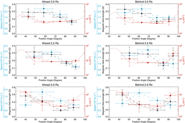
Figure 4. Magnetic field strengths (black) at heliocentric distances 2.0 (bottom), 2.5 (middle), and 3.0 R☉ (top) on the image planes taken from Ahead (left) and Behind (right), derived from speeds (blue) of the disturbance, electron densities (red), and a constant sound speed. The electron densities were measured with the SSI method. Abscissas are position angles as seen in Figures 1 and 2. The red solid curves represent the azimuthal profiles of the electron density. The red dashed lines with circles and vertical error bars refer to the averages and standard deviations over sections indicated by horizontal error bars. The horizontal error bars indicate sections where the disturbance passes through during the time intervals of the pB images.
Download figure:
Standard image High-resolution image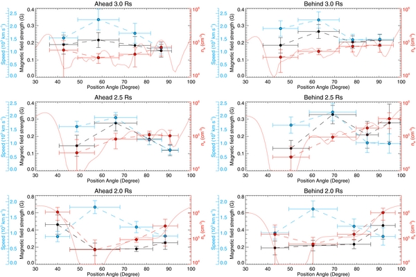
Figure 5. Same as Figure 4 but the electron densities were determined with the tomography method. In this case, we set the lower limit of the electron density 104 cm−3.
Download figure:
Standard image High-resolution imageIt is evident that the inhomogeneity of the density is responsible for the changes of the speeds. Since Alfvén speed may be much faster than sound speed in this height range, the speed of the disturbance vf ≈ vA, so that vf ∼  . A scatter plot of vf versus
  is shown in Figure 6 and indicates that the speeds are closely related to the densities. The correlation coefficient is 0.61.
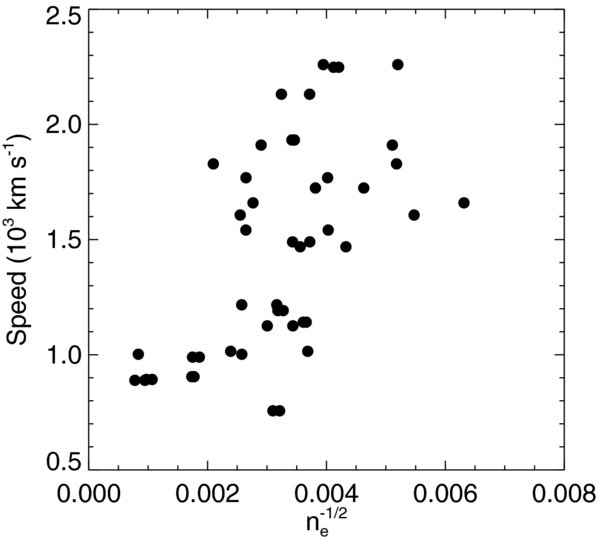
Figure 6. Scatter plots of speed vs.  . The correlation coefficient is 0.61.
Download figure:
Standard image High-resolution imageFigure 7 shows the full ranges of the inhomogeneous magnetic field strengths we obtained at 2.0, 2.5, and 3.0 R☉. The full ranges of the magnetic field strengths determined with the SSI method at the given heliocentric distances are 0.15–0.73, 0.09–0.38, and 0.12–0.41 G, respectively. In addition, the averages and standard deviations are 0.37 ± 0.15, 0.23 ± 0.07, and 0.24 ± 0.06 G, respectively. The averages and standard deviations determined with the tomography method are 0.27 ± 0.11, 0.21 ± 0.07, and 0.20 ± 0.03 G at the heliocentric distances, respectively. This figure shows that our results are mostly within values expected from empirical models (Dulk & McLean 1978; Mann et al. 1999; Gary 2001), determined with a different method (Mancuso et al. 2003), and determined with a PFSS model. We calculated global potential magnetic fields using the PFSS model (Altschuler & Newkirk 1969) with the source surface set at 2.5 R☉ and derived the radial profile of the magnetic field strength in the northern polar region, averaging over 30° around the northern rotational axis. These consistencies indicate that the determined magnetic field strengths are physically acceptable.

Figure 7. Radial profiles of magnetic field strength. The closed circles and error bars denote the averages and the full ranges of magnetic field strengths, respectively, determined with the SSI method. The ranges of magnetic field strengths determined with the tomography method are represented by crosses. The open circles refer to the ranges of magnetic field strengths determined in Kwon et al. (2013). The asterisks denote the magnetic field strengths determined with speeds of type II radio bursts (Mancuso et al. 2003). The dotted curves refer to an average of magnetic field strengths, determined with a PFSS model, over 30° around the solar rotational axis. Empirical profiles of magnetic field strengths above the quiet Sun (Mann et al. 1999) and an active region (Dulk & McLean 1978) are shown with dashed and dash-dotted curves, respectively. The solid curve refers to a modeled radial profile of magnetic field strength used for modeling plasma β above an active region (Gary 2001).
Download figure:
Standard image High-resolution imageFrom the determined physical parameters, electron density ne, and magnetic field strength B, and an assumed constant temperature T = (1.5 ± 0.5) × 106 K, we estimated plasma pressure, magnetic pressure, and plasma β at the various heliocentric distances. Plasma pressure can be determined with a relation pgas = 2nekBT, where kB is Boltzmann constant. We estimated magnetic pressure with a relation, pmag = B2/8π. The plasma β parameter is defined as a ratio of plasma pressure and magnetic pressure, β = pgas/pmag. Figure 8 shows the azimuthal profiles of the plasma β at the heliocentric distance of 2.0 (closed circles with solid lines) and 2.5 R☉ (open circles with dashed lines). The values at 3.0 R☉ are not so different from the ones at 2.5 R☉, and thus they are omitted from this figure. Plasma β parameters are found to be larger near coronal streamers. The averages and standard deviations over the entire paths on both image planes, Ahead and Behind, are listed in Table 1.

Figure 8. Azimuthal profiles of plasma β determined from the image planes taken from the COR1 Ahead (top) and Behind (bottom). The closed circles with solid lines denote the values determined at a heliocentric distance of 2.0 R☉ and the open circles with dashed lines refer to the values at 2.5 R☉.
Download figure:
Standard image High-resolution imageTable 1. Determined Physical Parameters
| Heliocentric Distance | 2.0 R☉ | 2.5 R☉ | 3.0 R☉ |
|---|---|---|---|
| 〈vf〉 (km s−1) | 1212 ± 360 | 1402 ± 466 | 1723 ± 369 |
| 〈ne〉 (cm−3) | (6.1 ± 5.9) × 105 | (1.2 ± 0.7) × 105 | (8.2 ± 3.0) × 104 |
| 〈B〉 (G) | 0.37 ± 0.15 | 0.23 ± 0.07 | 0.24 ± 0.06 |
| 〈pgas〉 (dyne cm−2) | (2.5 ± 2.4) × 10−4 | (5.1 ± 2.8) × 10−5 | (3.4 ± 1.2) × 10−5 |
| 〈pmag〉 (dyne cm−2) | (6.2 ± 4.5) × 10−3 | (2.4 ± 1.3) × 10−3 | (2.4 ± 1.1) × 10−3 |
| 〈β〉 | (3.6 ± 1.6) × 10−2 | (3.1 ± 2.1) × 10−2 | (1.6 ± 0.7) × 10−2 |
Notes. Rows are as follows: the averages and standard deviations of the determined parameters, the fast magnetosonic speed vf, electron density ne, magnetic field strength B, plasma pressure pgas, magnetic pressure pmag, and plasma β.
Download table as: ASCIITypeset image
Figure 9 shows the full ranges of the determined plasma pressure, magnetic pressure, and plasma β, and comparisons with previous works (Li et al. 1998; Gary 2001; Mancuso et al. 2003; Kwon & Chae 2008; West et al. 2011). The left panel shows the plasma and magnetic pressures with black and gray horizontal bars, respectively, and that the magnetic pressure is higher than the plasma pressure at the heliocentric distances 2.0, 2.5, and 3.0 R☉. The dashed curve represents a widely accepted modeled plasma pressure profile over an active region (Gary 2001) and these values tend to be higher than the plasma pressure we determined and lower than the determined magnetic pressure. The plasma pressures we found are lower than the ones in a coronal helmet streamer at 1.15 and 1.5 R☉ (Li et al. 1998) and in coronal loops observed by TRACE 171 Å (Kwon & Chae 2008). The plasma β parameters (black bars) are lower than the values modeled over an active region (dashed curves; Gary 2001). They are also lower than the values determined in a coronal helmet streamer (asterisks; Li et al. 1998), an active region corona (closed circle; Mancuso et al. 2003), and quiet Sun corona (open circle; West et al. 2011).
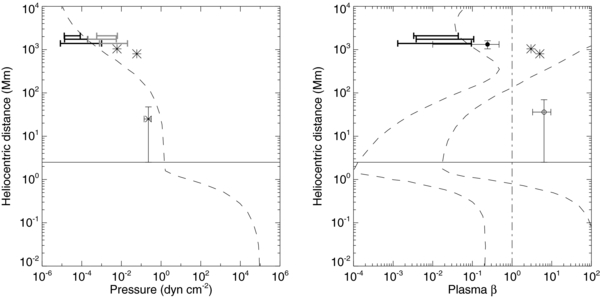
Figure 9. Radial profiles of pressures and plasma β. The horizontal solid lines in both panels refer to the typical height of the lower boundary of the solar corona, 2.5 Mm. The dashed curves denote plasma pressure (left panel) and plasma β (right) above an active region, modeled in Gary (2001). In the left panel, thick black and gray error bars represent the full ranges of plasma pressure and magnetic pressure, respectively, determined in the present work, at heliocentric distances 2.0, 2.5, and 3.0 R☉. The asterisks are plasma pressure in a coronal helmet streamer determined at 1.15 and 1.5 R☉ (Li et al. 1998). The "x" with error bars represents plasma pressure on coronal loops observed by TRACE 171 Å (Kwon & Chae 2008). In right panel, thick black error bars show the full ranges of plasma β determined in the present work at the heliocentric distances. The closed circle refers to plasma β in a heliocentric distance range of 1.5–2.3 R☉ in coronal streamers above coronal active regions (Mancuso et al. 2003). The asterisks are plasma β in a coronal helmet streamer determined at 1.15 and 1.5 R☉ (Li et al. 1998). The open circle and error bars represent plasma β determined with kinematics of an EIT wave in the low solar corona (West et al. 2011). The vertical dash-dotted line denotes the unity of plasma β.
Download figure:
Standard image High-resolution imageTable 1 lists the determined physical parameters with the corresponding standard deviations, at the heliocentric distances 2.0, 2.5, and 3.0 R☉. The parameters are averaged over the entire trajectories of the disturbance on both image planes taken from Ahead and Behind. Since the electron densities determined with the tomography method contain unrealistic values at some azimuthal points, we show only the electron densities and magnetic field strengths determined with the SSI method.
4. DISCUSSION
By applying the speed of a fast magnetosonic wave and the electron densities determined from observations to Equation (1), we found that the inhomogeneous magnetic field strength varied with the azimuthal and radial directions in the extended solar corona. Note that a propagating front should be well established as a true wave front and the physical properties of the wave should be theoretically well understood. In order to meet these requirements, we used kinematics of the disturbance well established as a true fast magnetosonic wave in Paper I. For simplicity, possible effects of wave reflection, trapping, and dispersion are neglected (see Liu et al. 2012; Paper I for examples of these effects associated with fast magnetosonic waves observed by SDO, EUVI, and COR1 coronagraphs). There is an uncertainty in representing the true magnetic field strength in this method. This comes from the fact that the speeds and densities are the averages over the trajectories of the wave front and that the medium along the trajectories may not be homogeneous. Note that Equation (1) is based on a linear dispersion relation and is strictly valid for a homogeneous medium. This relation may not hold when averaging each quantity over an inhomogeneous medium. In this paper, we simply chose only parts of the wave trajectories between two streamers as seen in Figure 1 and postulated that the medium within the individual sections in which the disturbance travels during the time intervals of the observations is nearly homogeneous and that the disturbance is a linear wave or weakly shocked, implying that the Mach numbers are close to unity. This assumption is supported by the fact that the amplitude of the disturbance dn/n ∼ dB/B is small. Instead, we estimated the uncertainty of the magnetic field strength δB by calculating the propagation error using the range of the mass density Δρ determined within the each section and the uncertainty of the speed δvf. According to this approach, the determined ranges of magnetic field strength, B ± δB, may cover the true values.
4.1. Physical Parameters
The independent and simultaneous observations of the twin STEREO spacecrafts may allow us to determine an uncertainty in determining the magnetic field strength B, which is caused by measurement errors in speed vf and density ρ. Note that vf and ρ are determined independently from the two image planes taken from the COR1 Ahead and Behind. The difference in the retrieved values from the two image planes may be due to a combination of the intrinsic differences of the coronal medium observed by the two spacecraft and the measurement errors in vf and ρ. In this context, it may give us the maximal measurement error. The left panel in Figure 10 shows the difference of B determined from the two image planes. The difference is about 30% of the determined values, indicating that the measurement error is less than 30%. On the other hand, the right panel in this figure shows the comparison between B determined with ρ derived from the SSI and the tomography methods. In this case, the difference of B is about 40%. This difference may indicate the uncertainty in measuring B due to assumptions for the calculations of electron density. In addition, the propagation error in B (vertical error bars in Figure 4) is about 25%, which is less than the above uncertainties. This analysis demonstrates that our method allows us to determine magnetic field strength with an uncertainty less than 40%.

Figure 10. Scatter plots of magnetic field strengths. The left panel shows difference of magnetic field strengths determined from the two different image planes taken from Ahead and Behind. The difference between magnetic field strengths determined through the SSI and tomography methods is shown in the right panel.
Download figure:
Standard image High-resolution image
For the first time, we showed the variation of the magnetic field strength B across magnetic field lines in the azimuthal direction in a wide spatial range of the extended solar corona and the full ranges of B varying in the azimuthal direction at the heliocentric distances are 0.15–0.73, 0.09–0.38, and 0.12–0.41 G, respectively. This indicates that the magnetic field strengths at given heliocentric distances vary in 66%, 65%, and 54% with respect to their median values. The changes in B in the azimuthal direction may be physically significant since the uncertainty in determining B is less than 40%. Note that our analysis partially covers streamers. The azimuthal profiles of B in Figure 4 imply that B on the axes of the streamers should be larger than what we found near the axes and B at a given heliocentric distance may vary much more than what we showed above. Dulk & McLean (1978) showed that B can vary about 2 orders of magnitude depending on coronal regions at a given heliocentric distance.
The average and full range of B at 3.0 R☉ are slightly higher than those at 2.5 R☉ (Figure 7), which may be due to a combination of the slow decreasing rate of B with height and an artificial effect. First of all, it is likely that B may drop off slowly above the coronal hole. In case the magnetic field expands freely from a homogeneous spherical source, one may expect that B falls off with a rate of r−2, where r is the radial distance from the center of the spherical source, as seen in an empirical model above the quiet Sun (Mann et al. 1999). Undoubtedly, in reality, the magnetic field in the solar corona will expand with a different rate due to the inhomogeneity of the photospheric magnetic fluxes and the existence of currents. If one determines the radial profile of B above a confined strong source region (active region) in the low solar corona, B will decrease faster than the rate of r−2, as seen in an empirical model above an active region (Dulk & McLean 1978). As for a region between two confined strong source regions, B would decline slower than the rate of r−2 (e.g., current sheet region; Gary 2001). In this study, B ∝ r−1.3, consistent with a rate determined in a heliocentric distance ranging from 6 to 23 R☉ (Gopalswamy & Yashiro 2011). As discussed above, the region we analyze here is the coronal hole surrounded by regions where B is stronger. The stronger magnetic field strength in the surroundings seen in Figure 4 may be responsible for the slowly decreasing B in this region. For this reason, the true magnetic field strength at 2.5 and 3.0 R☉ may not be so different.
Second, the density ρ at 3.0 R☉ may be overestimated and the higher ρ may introduce the overestimated B, since B ∝ ρ1/2 in Equation (1). It is well known that ρ in the low solar corona falls off quickly in the radial direction and, especially, most of the region is composed of the polar coronal hole where ρ is very low. Due to this effect, the noise of the pB images may be considerable at 3.0 R☉ in this region (see Thompson et al. 2010 for detailed descriptions of the calibration method for the COR1 coronagraphs). Note that the signal-to-noise ratio of the COR1 images in the denser coronal structures, such as the quiet Sun/active region corona, streamers, and plumes, may be high enough to measure the correct electron density above the heliocentric distance of 3.0 R☉ (Thompson et al. 2010).
The speeds of the fast magnetosonic wave vf increase with height and they are 1212 ± 360, 1402 ± 466, and 1723 ± 369 km s−1 at 2.0, 2.5, and 3.0 R☉, respectively (Paper I), and the increasing tendency is consistent with the modeled radial profiles of vf and vA (Alfvén speed) above the quiet Sun (Mann et al. 1999, 2003; Gopalswamy et al. 2001). These models show that vf or vA in the quiet Sun corona has a peak around 3–4 R☉ and the maximum speed is 500–800 km s−1 (cf. Régnier et al. 2008 for the profile of vA above an active region) and that this speed is slower than what we found at 2.0 R☉. In addition, the average increasing rate of the speed with height, Δvf/Δr, we found is ∼500 km s−1  and it is steeper than the expected rate with the models, which is 100–300 km s−1
  . The faster speed and steeper increasing rate could be explained by the characteristics of the medium in the coronal hole: low ρ and slowly declining B. These characteristics may introduce the faster local vf and the steeper profile than what the models show. This discussion indicates that the radial profile of vf above the coronal hole is similar to the ones in the quiet Sun corona but the speed is faster and the profile is steeper.
It is important to note that vf does not show significant correlation with B. Yang & Chen (2010) found negative correlations between the speeds of EIT waves and magnetic field strengths determined with a potential field model. This fact has been considered as a convincing argument that EIT waves are not fast magnetosonic waves at all. As seen in Figure 4, however, B is stronger in coronal streamers than in a coronal hole region, but vf is slower in the coronal streamers. This is caused by highly inhomogeneous density distribution. Suppose a constant sound speed, vf, is proportional to Alfvén speed,  . In case
  changes rapidly much faster than B, vf would be correlated with
  rather than B. In this respect, the speeds of EIT waves may not be correlated with B. In this work, the correlation coefficients between vf versus
  and vf versus B are found to be 0.61 (Figure 6) and −0.02, respectively.
We determined plasma β parameters at the heliocentric distances 2.0, 2.5, and 3.0 R☉ and they are found to be significantly lower than previous results (Li et al. 1998; Gary 2001; Mancuso et al. 2003), as seen in Figure 9. Li et al. (1998) determined the temperature and electron density of a coronal streamer at heliocentric distances of 1.15 and 1.5 R☉ using Yohkoh SXT and SOHO UVCS and derived β together with the magnetic field strength determined with a PFSS model. The determined β parameters are 5 and 3 at the heliocentric distances, respectively (asterisks in right panel of Figure 9). Mancuso et al. (2003) estimated the magnetic field strength by analyzing a number of metric type II radio bursts and electron density using SOHO UVCS. Using the determined B and ne, they provided β ∼ 0.3 around 1.9 R☉ in streamers. These two results are consistent with the modeled β by Gary (2001) as seen in Figure 9 (dashed curves). Gary (2001) showed that β increases from about 10−4–10−2 at the coronal base to ∼1 around 1.2 R☉ (see also Régnier et al. 2008) and pointed out that the layer where β < 1 is surrounded by the layers where β > 1. Note that these estimates are for streamers above active regions while our measurements are done mostly in the polar coronal hole. As shown in the left panel in Figure 9, the plasma pressures we found are significantly lower than the values reported by Li et al. (1998, asterisks) and Gary (2001, dashed curve). The azimuthal profiles of β in Figure 8 demonstrate that the coronal hole is lower in β than streamers. These facts imply that the low plasma β parameters in these heliocentric distances are valid in the coronal hole region.
One may discern from the above discussions that β should decrease with height in the quiet Sun corona and coronal hole, unlike an active region shown by Gary (2001). It has been widely accepted that vf or vA increases with height in the quiet Sun corona (Mann et al. 1999, 2003; Gopalswamy et al. 2001; Evans et al. 2008) and those profiles are consistent with observations and interpretations of various manifestations of fast magnetosonic waves or shocks (Uchida 1968; Mann et al. 1999, 2003; Gary 2001). These profiles suggest that β should decrease with height until around 4 R☉, where vf and vA have their maxima, since β can be expressed by the ratio between the sound speed and Alfvén speed; that is β = 2(cs/vA)2 assuming γ = 1. In this study, we only cover a heliocentric distance range from 2.0 to 3.0 R☉, but we can simply estimate β in the lower solar corona, considering speeds of EIT waves. For instance, West et al. (2011) estimated β using an observed EIT wave and found that β = 6.4 ± 3.1 (vf = 220 ± 30 km s−1). Ballai (2007) determined the magnetic field strength, electron density, and temperature with kinematics of an EIT wave and these values give β ranging 0.3–2.4 (vf = 250 and 400 km s−1). As a matter of fact, it has been highly debated whether or not that EIT waves are in fact fast magnetosonic waves. Recently, it has been widely accepted that an EIT wave front consists of two fronts, true wave front and pseudo-wave front. In order to find the true wave speed range, we only consider the cases whose the two components are clearly detected simultaneously (Asai et al. 2012; Chen & Wu 2011; Ma et al. 2011; Olmedo et al. 2012). The speeds of the wave components range from 300 to 700 km s−1. Assuming that cs is 200 km s−1, vA derived from the observed speed range is ranging from 220 to 670 km s−1. By applying this range to the above relation, we have β ranging from 0.2 to 1.7, indicating that β is close to unity in the corona close to the Sun. These values are significantly higher than what we found at 2.0, 2.5, and 3.0 R☉. Together with these estimates and the modeled profiles of vf and vA, we may conclude that β decreases with height above the quiet Sun and coronal hole, unlike the medium above active regions.
4.2. Physical Implications
Together with prior knowledge, the results of our coronal seismology allow us to explain some observational characteristics of waves or shocks, which have not been fully understood. Since previous interpretations of manifestations of waves or shocks associated with CMEs have been done based on modeled physical quantities (Uchida 1968; Mann et al. 1999, 2003; Gopalswamy et al. 2001; Warmuth & Mann 2005; Evans et al. 2008; Yang & Chen 2010), the interpretations should be verified with measured physical quantities.
The azimuthal and radial profiles of ρ, B, and β we determined are consistent with interpretations of Moreton and EIT waves. Fast magnetosonic waves may be initiated in the form of strong shock (pressure pulse) with a shape of sphere (Veronig et al. 2010; Cheng et al. 2012; Liu et al. 2012; "Paper I"), expanding faster than the local vf, and then fast magnetosonic wave will propagate in all directions into the ambient corona from the spherical shock front. Because of the fast declining ρ with height, the local vf rises rapidly, even if B decreases with height, so that the driven fast magnetosonic wave will be refracted toward the lower altitude. The refracted wave front may reach the chromosphere through the low solar corona and form a shock due to the dense medium in this layer.
According to this scenario, EIT waves are downward-propagating fast magnetosonic waves refracted from the upper solar corona, similar to the interpretation of Moreton waves (Uchida 1968), rather than freely propagating fast magnetosonic waves confined to a certain coronal layer. As shown by our coronal seismology and previous studies, the coronal medium is highly inhomogeneous and a wave propagating in this medium must be refracted. In case vf increases or decreases with height, a freely propagating wave in a certain coronal layer will disappear quickly because of the refraction toward the chromosphere or the upper solar corona, respectively. The only way to show continuous fronts propagating against the layer is that the wave or shock front propagating in the upper solar corona should be refracted toward the lower atmospheric layer and disturbs the plasma in the low corona and chromosphere. This idea is supported by a spectroscopic result of an EIT wave (Veronig et al. 2011). Veronig et al. (2011) found down-up motion of plasma in the LOS direction at the front of an EIT wave, which means that the direction of the local compression and rarefaction of plasma is inclined toward the solar surface. In the same context, this scenario provides a clue to understanding why some flares do not show EIT waves and why some EIT waves do not propagate isotropically against the low coronal layer. If a wave front or part of a wave front passes through a region where vf decreases with height, as seen in the profile above an active region, the wave front will be refracted upward and then the wave front may not reach the low corona.
The profiles of the physical parameters in the radial and azimuthal directions are consistent with previous interpretations of coronal shocks through modeled profiles (Mann et al. 1999, 2003; Gopalswamy et al. 2001; Evans et al. 2008). Gopalswamy et al. (2001 and references therein) used modeled profiles of vf for the active region and the quiet Sun corona and tried to explain the short lifetime (or short traveling distance) of metric type II radio bursts (see also Mann et al. 1999, 2003). They found very high vf at the coronal base and rapidly declining profile with height in the active region corona and the lower vf at the coronal base and increasing profile in the quiet Sun corona. According to their explanation, metric type II radio bursts may be formed when CME's ejecta cross over from the active region corona (high vf) to the quiet Sun corona (low vf) and the shock will disappear quickly because the local vf increases rapidly with height in the quiet Sun corona. The radial profiles of the physical parameters we found support this scenario of the short lifetime of metric type II radio bursts.
The azimuthal profiles of vf imply that local dense structures, such as coronal streamers, may be responsible for multiple shocks driven by a single source (cf. Evans et al. 2008). Figure 4 shows that vf is significantly lower in streamers than the surroundings, even if B is stronger, and implies that the azimuthal components of outgoing CME ejecta and/or the driven fast magnetosonic waves can be easily shocked in these regions. This idea is consistent with reports on multiple type II radio bursts (Cho et al. 2011; Feng et al. 2013) and discontinuous signals of type II radio bursts (Feng et al. 2012, 2013; Kong et al. 2012) caused by CME-streamer interactions.
Kahler & Reames (2003 and references therein) looked for important factors to generate gradual SEP events by shocks associated with CMEs: the speed of CMEs and the apparent angular width of CMEs. They found a very low probability of triggering SEP events above coronal hole regions due to the high local vf expected in these regions. These findings and explanations are consistent with our measurements that the region above the coronal hole is much higher in vf than the surroundings and that vf increases rapidly with height. In addition, the apparent angular widths of CMEs were found to be one of the important factors, indicating that the CME components propagating in the azimuthal direction may be efficient to generate gradual SEP events with the perpendicular shocks due to the interactions with radial coronal structures where vf is lower than the surroundings. It is also pointed out by Gopalswamy et al. (2001) that CMEs with wider angular widths may have a higher probability of becoming shocked. Our results of global coronal seismology support the scenario that gradual SEP events are generated by shocks due to the azimuthal components of CMEs, passing through radial coronal structures, such as streamers, where vf is lower than the surroundings.
5. CONCLUSIONS
We determined the magnetic field strength along the azimuthal trajectories of a disturbance, which has been well-established as a true fast magnetosonic wave in Paper I, at heliocentric distances 2.0, 2.5, and 3.0 R☉. The uncertainty was found to be less than 40% of the determined values. The characteristics of the coronal medium revealed with global coronal seismology are that (1) the density, magnetic field strength, and plasma β are lower in the coronal hole region than in streamers; (2) the magnetic field strength decreases slowly with height but the electron density decreases rapidly so that the local fast magnetosonic speed increases while plasma β falls off with height; and (3) the variations of the local fast magnetosonic speed and plasma β are dominated by variations in the electron density rather than the magnetic field strength. These characteristics of the coronal medium imply that Moreton and EIT waves are downward-propagating fast magnetosonic waves or shocks refracted from the upper solar corona, rather than freely propagating fast magnetosonic waves in a certain solar atmospheric layer. In addition, the azimuthal components of CMEs and the driven waves may play an important role in various manifestations of shocks, such as type II radio bursts and SEP events.
Due to the high time cadence white light observations by the STEREO COR1 inner coronagraphs, fast magnetosonic waves propagating in the extended solar corona became directly observable. Accordingly, their geometric and kinematic properties are directly measured and used for global coronal seismology. The coronal seismology method we present here provides a unique way to diagnose an inhomogeneous medium in a broad range of the extended solar corona, systematically and straightforwardly. The characteristics of the local coronal medium vary significantly with the solar cycle and regions. In this instance, the time of this event corresponds to a period approaching the maximum of solar cycle 24th and the fast magnetosonic wave propagates mainly in a polar coronal hole and partially in streamers. We plan to extend our study to a sizable sample of fast magnetosonic waves associated with CMEs using white light observations, to study distributions of magnetic field strength in the extended solar corona.
R.-Y.K. and L.O. acknowledge support by the NASA grant NNX10AN10G. L.O. acknowledges support by NASA grants NNX12AB34G and NNX11AO68G. The work of T.W. was supported by the NASA cooperative agreement NNG11PL10A to CUA and the NASA grant NNX12AB34G.