


ABSTRACT
We performed simple spot-model calculations for quasi-periodic brightness variations of solar-type stars showing superflares using Kepler photometric data. Most of the superflare stars show quasi-periodic brightness modulations with a typical period of one to a few tens of days. Our results indicate that these brightness variations can be explained by the rotation of a star with fairly large starspots. Using the results of the period analysis, we investigated the relation between the energy and frequency of superflares and the rotation period. Stars with relatively slower rotation rates can still produce flares that are as energetic as those of more rapidly rotating stars although the average flare frequency is lower for more slowly rotating stars. We found that the energy of superflares is related to the total coverage of the starspot. The correlation between the spot coverage and the flare energy in superflares is similar to that in solar flares. These results suggest that the energy of superflares can be explained by the magnetic energy stored around the starspots.
Export citation and abstract BibTeX RIS
1. INTRODUCTION
Solar flares are the most energetic explosions on the surface of the Sun and are thought to be caused by the release of magnetic energy (e.g., Shibata & Magara 2011). Flares are also known to occur on various types of stars, including solar-type ones (Schaefer 1989; Gershberg 2005). Among the solar-type stars, young stars and close binary stars sometimes produce "superflares," which have a total energy 10–106 times more (∼1033–38 erg; Schaefer et al. 2000) than the largest flares on the Sun (∼1032 erg). Such stars generally rotate fast (vrot ∼ a few 10 km s−1), and magnetic fields of a few kG are distributed in large regions on the stellar surface (Gershberg 2005; Shibata & Yokoyama 1999, 2002). In contrast, the Sun rotates slowly (vrot ∼ 2 km s−1) and the magnetic fields are weak. Here, we define "Sun-like" stars as solar-type stars that rotate slowly and whose surface temperature is 5600–6000 K. It was once thought that superflares cannot occur on Sun-like stars.
Schaefer et al. (2000), however, found nine superflare candidates on slowly rotating Sun-like stars. This is extremely important in many fields, including magnetic activity research in solar/stellar physics as well as planetary habitability in astrobiology (e.g., Segura et al. 2010). The frequency, detailed properties, and mechanism of superflares are, however, still not clear because of a lack of observations. Therefore, it is necessary to investigate them in detail to determine their properties how often they occur on solar-type stars, and the stellar conditions that lead to their formation.
We have already analyzed the data from the Kepler spacecraft (Koch et al. 2010) and discovered 365 superflare events on 148 solar-type stars that have a surface temperature of 5100 K ⩽ Teff < 6000 K and a surface gravity of log g ⩾ 4.0 (Maehara et al. 2012). The Kepler spacecraft is very useful in detecting faint increases in stellar brightness caused by stellar flares, because Kepler observed with high photometric precision and obtained continuous time-series data of many stars over a long period (Walkowicz et al. 2011; Balona 2012). We found that superflares with energy 102–103 times higher than that of the most energetic flare on the Sun can occur on solar-type stars once in a few thousand years. Many solar-type stars with superflares show quasi-periodic brightness variations with a typical period of one day to a few tens of days. Such variations can be explained by the rotation of the star (e.g., Basri et al. 2011; Debosscher et al. 2011; Harrison et al. 2012).
In this paper, we investigate the brightness variations of superflare-generating stars by considering the signature of stellar rotation and starspots. First, we use a simple model analysis to show that the brightness variation of some typical superflare-generating stars can be explained by the rotation of a star with starspots. The main purpose of the model analysis is to demonstrate that the brightness variations contain information about the overall area coverage of the starspots and the rotation periods of superflare stars. Second, using the results of the period analysis, we consider the relationship between the rotation period and properties of superflares such as flare energy and flare frequency. Third, we discuss the relationship between the starspot coverage and the energy of superflares by assuming that the brightness variations are due to the rotation. For the Sun, we know that there is a positive correlation between the sunspot coverage and the energy of the largest flare observed, and that the energy of the largest flare depends on the magnetic energy stored around the sunspots (e.g., Sammis et al. 2000). We then investigate whether this correlation can be applied to superflare-generating stars, and discuss the relationship between the magnetic energy of the starspots and the superflare energy.
The details of the Kepler data that we use in this paper are explained in Section 2. We show the results of spot modeling for some typical superflare-generating stars. In Section 4, we consider the relationship between the rotation period and the superflare properties based on the results of the period analysis. In Section 5, we discuss the relationship between the starspot coverage and the energy of superflares by assuming that the brightness variations of superflare-generating stars are due to the rotation.
2. OBSERVATIONAL DATA AND PERIOD ANALYSIS
We searched for flares on solar-type stars using the Kepler data that were obtained from 2009 April to 2010 September (Quarters 0–6). These data were retrieved from the Multimission Archive at Space Telescope Science Institute.5 We used the effective temperature (Teff) and the surface gravity (log g) in the Kepler Input Catalog (Brown et al. 2011) to select solar-type stars. The selection criteria are as follows: 5100 ⩽ Teff < 6000 and log g ⩾ 4.0. The total number of solar-type stars is about 90,000. The length of the observation period during each quarter and the number of solar-type stars are summarized in Table 1.
Table 1. Length of the Observation Period During Each Quarter and the Number of Solar-type Stars
| Quarter | Na | τb | Releasec |
|---|---|---|---|
| (days) | |||
| 0 | 9511 | 11 | 14 |
| 1 | 75598 | 33 | 14 |
| 2 | 82811 | 90 | 14 |
| 3 | 82586 | 90 | 14 |
| 4 | 89188 | 90 | 14 |
| 5 | 86248 | 95 | 16 |
| 6 | 82052 | 90 | 16 |
Notes. aNumber of solar-type stars. bLength of the observation period during each quarter. cKepler data release numbers for the data we use in this paper. dKepler Data Release 14 Notes (Christiansen & Barclay 2012a). eKepler Data Release 16 Notes (Christiansen & Barclay 2012b).
Download table as: ASCIITypeset image
We analyzed the long-cadence (time resolution of about 30 minutes) flux detrended by the PDC-MAP pipeline (Stumpe et al. 2012) to detect superflares. Details on the detection method are described in Maehara et al. (2012) and Shibayama et al. (2013). The version of the data we use in this paper is shown in Table 1.
Figure 1 shows typical light curves of solar-type stars with superflares (KIC 6034120 and KIC 6691930, Quarter 2; KIC 10528093, Quarters 0–2). KIC 6034120 shows a light curve with a simple sine-like profile that can be reproduced well with one large starspot. The light curve of KIC 6691930 requires two starspots to explain the shoulder of the rising part. KIC 10528093 also needs two starspots, and its long-term amplitude variation cannot be explained by the solid rotation model. These data are selected to clearly demonstrate these features. The light curves of all solar-type stars with superflares reported in Shibayama et al. (2013) are shown in Figure 11. The period of the brightness variation was estimated using the discrete Fourier transform method. We carried out the following five procedures. (1) We measured the standard deviations (σ) of the data in each quarter and deleted all the data from any quarter whose σ value was over three times larger than the mean value. (2) The linear trend was removed from the brightness each quarter. (3) The gaps in the mean brightness between each quarter were adjusted. (4) We took the power spectra of the period from 0.1 days to 45 days, since the reduction pipeline seems to generate spurious peaks at timescales longer than 45 days, which is half the typical length of each quarter.6 (5) We chose the peak from the power spectrum whose amplitude had the highest ratio to the red noise spectrum (e.g., Press 1978; Vaughan 2005) to be the period of the brightness variation of the star, since in some cases simply taking the highest peak can lead us to choose spurious peaks at long timescales. Figure 2 shows the results of the period analysis for the brightness variations shown in Figure 1. Such stars show quasi-periodic brightness variations with a typical period of one day to a few tens of days.

Figure 1. Light curves of typical superflares on solar-type stars (KIC 6034120 and KIC 6691930, Quarter 2; KIC 10528093, Quarters 0–2). The vertical axis shows the brightness variations relative to the average brightness. The typical photometric error is about 0.02%. The arrows indicate superflares reported in Maehara et al. (2012).
Download figure:
Standard image High-resolution image
Figure 2. Power spectra of the light curves shown in Figure 1. The periods of these three stars are shown in Table 2.
Download figure:
Standard image High-resolution image3. MODEL CALCULATION OF THE BRIGHTNESS VARIATION OF ROTATING STARS WITH LARGE STARSPOTS
We performed simple calculations to show that brightness variations of superflare-generating stars can be explained by their rotation and the presence of large starspots. There are many previous studies that calculate the brightness variation by assuming the existence of dark spots on the surface of the star (e.g., Budding 1977; Dorren 1987; Eker 1994). Spot modeling has a lot of uncertainty and it is almost impossible to obtain unique solutions (e.g., Eker 1996; Kovari & Bartus 1997; Walkowicz et al. 2013). There are many parameters such as the inclination angle and the spot latitude that affect the shape of the light curve. In addition, the Kepler spacecraft provides only single-color photometry data, and this also creates degeneracy between the spot size and the spot contrast. Our main purpose is to demonstrate that the brightness variations provide information about the overall starspot area coverage and the rotation periods of superflare stars.
Our method of spot modeling is as follows. We consider the total luminosity of the photosphere and the starspot area to be a good representation of the flux (F) in our modeling. The shape of the model star is assumed to be a sphere, and some circular spots are placed on the photosphere. It should be noted that we do not exclude the possibility that starspots on superflare stars are collections of smaller spots. The surface of the star is divided into 180 pieces (j) latitudinally and into 360 pieces (k) longitudinally. The contributions to the total brightness are summed up from each piece (fj, k) as follows:
where
The temperature of the photosphere (Tphot) and that of the spot area (Tspot) are considered here to be the same over the solar photosphere (6000 K) and the sunspot area (4000 K; see Berdyugina 2005), respectively. The luminosity of each piece in the starspot area is estimated by

where Spix and nj,k are the size and the normal vector of each pixel, respectively, aj,k is a unit vector that is antiparallel to the line of sight, and σSB is the Stefan–Boltzmann constant. The luminosity of each piece that is out of the starspot area is estimated by
We also take into account the effect of limb darkening. Applying Equation (1) from Sing (2010), this effect is calculated by

where  is the luminosity of each piece without the limb-darkening effect, fj, k(μ) is the luminosity with the limb-darkening effect and μ = cos Θ with Θ the viewing angle. Here we assume u = 0.6 on the basis of Figure 3 in Claret (2004). Due to the rotation, the visibility of the starspots changes and the brightness varies. We calculate the brightness by changing the angle of rotation by 1°. Model light curves are drawn by arbitrarily changing the spot position, spot radius, and inclination angle i, which is the angle between the line of sight and the rotation axis of the star. We selected cases that show a rough agreement between the model and the observation by eye.
Figures 3–5 show the results of the spot-model calculation for the brightness variations of typical solar-type stars with superflares shown in Figure 1 (KIC 6034120, KIC 6691930, and KIC 10528093). The stellar parameters of these stars are shown in Table 2. The period of the brightness variations is about 5–15 days, and the amplitude is from 0.1% to a few percent.
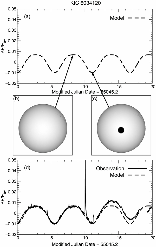
Figure 3. (a) Model light curve for KIC 6034120 (Figure 1(a)). The model parameters are given in Table 3. (b) and (c) Model images of the visible area of the photosphere with a starspot. (d) Observed light curve (solid line; the same as in Figure 1(a)) and model light curve (dashed line) for KIC 6034120.
Download figure:
Standard image High-resolution image
Figure 4. (a) Model light curve for KIC 6691930. The model parameters are given in Table 3. (b) and (c) Model images of the visible area of the photosphere with two starspots. (d) Observed light curve (solid line; the same as in Figure 1(b)) and model light curve (dashed line) for KIC 6691930.
Download figure:
Standard image High-resolution image
Figure 5. (a) Model light curve for KIC 10528093. The model parameters are given in Table 3. (b)–(e) Model images of the visible area of the photosphere with starspots. (f) Observed light curve (solid line; the same as in Figure 1(c)) and model light curve (dashed line) for KIC 10528093.
Download figure:
Standard image High-resolution imageTable 2. Stellar Parameters for Three Solar-type Superflare-generating Stars
| Kepler ID | Teffa | log ga | R/R☉a | Periodb | Amplitudec |
|---|---|---|---|---|---|
| 6034120 | 5407 | 4.7 | 0.77 | 5.6 | 4.45 × 10⁻³ |
| 6691930 | 5348 | 4.5 | 0.95 | 13.1 | 1.29 × 10⁻² |
| 10528043 | 5143 | 4.5 | 0.88 | 12.9 | 6.52 × 10⁻³ |
Notes. Model analysis results for these stars are shown in Figures 4–6. aThese data are taken from the Kepler Input Catalog (Brown et al. 2011). bThe period of the largest amplitude component of the brightness variation in units of days. cThe normalized amplitude of the dominant period.
Download table as: ASCIITypeset image
As shown in Figure 3, the simple sine-like light curve of KIC 6034120 can be reproduced by the model with one spot. Figure 3(a) shows the model light curve for KIC 6034120. The best set of model parameters is listed in Table 3. Snapshots of the modeled star are displayed in Figures 3(b) and (c), which shows that the star has a larger spot than the Sun. Figure 3(d) shows the comparison of the observed light curve with the model light curve.
Table 3. Best Set of Model Parameters for Figures 3–5
| Kepler ID | Inclination | Spot Name | Rspot/Rphot | Initial Latitude | Initial Longitude Difference |
|---|---|---|---|---|---|
| 6034120 | 45° | Spot1 | 0.13 | 41°N | ⋅⋅⋅ |
| 6691930 | 32° | Spot1 | 0.23 | 30°N | ⋅⋅⋅ |
| ⋅⋅⋅ | ⋅⋅⋅ | Spot2 | 0.21 | 60°N | 70° |
| 10528043 | 60° | Spot1 | 0.15 | 0°N | ⋅⋅⋅ |
| ⋅⋅⋅ | ⋅⋅⋅ | Spot2 | 0.10 | 37°N | 120° |
Download table as: ASCIITypeset image
The light curve of KIC 6691930 has one peak and one shoulder, as shown in Figure 1(b). The features can be reproduced by the two-spot model as shown in Figure 4. The longitudinal difference between the two spots can be estimated by measuring the rotational phase of the shoulder in the light curve. Figure 4(a) shows the model light curve for KIC 6691930. The model parameters are listed in Table 3. Figures 4(b)–(d) are drawn for KIC 6691930 in the same manner as Figures 3(b)–(d) for KIC 6034120.
The light curve of KIC 10528093 also has a shoulder, as shown in Figure 1(c). However, the long-term amplitude variation cannot be reproduced by a simple model with two spots in solid body rotation, because the phase of the shoulder changes as time progresses.
These variations can be explained by differential rotation (e.g., Frasca et al. 2011; Fröhlich et al. 2012). Here, we consider the two-spot model with differential rotation. It should be noted that the differential rotation in this model is only approximately the correct amount. This is because a qualitatively similar fit would be produced by model with almost any spot parameters that obtains the correct differential rotation and the rough longitudinal separation. Parameters of the differential rotation (the dependence of the rotation speed on the latitude) that we use here are based on the Sun's values (Snodgrass & Ulrich 1990). The relationship between the angular velocity of the rotation (ω) and the latitude (φ) is represented by

For the Sun, A = 14 71 day−1, B = −239 day−1, and C = −178 day−1 (Snodgrass & Ulrich 1990). Here, we ignore the "Csin 4φ" term since it is negligibly small in our model, and then we convert the A and B values to ones that correspond to the rotation period of KIC 10528093. For KIC 10528093, the values of A and B are A = 311 day−1 and B = −505 day−1. Figure 5(a) shows the model light curve for KIC 10528093. The model parameters are listed in Table 3. Snapshots of the modeled star are shown in Figures 5(b)–(e). We compare the observed light curve with the modeled light curve in Figure 5(f). Figure 6 shows power spectra of the observed and model light curves shown in Figure 5(f). We can see that features of the power spectrum, i.e., the dominant and overtone peaks and the slope to the higher frequencies, are also roughly reproduced with our spot model.

Figure 6. Power spectra of the period analysis for the observed and model light curves of KIC 10528093 shown in Figure 5(f).
Download figure:
Standard image High-resolution imageMost of the brightness variations with a period of a few days to a few tens of days and an amplitude of 0.1%–10% are expected to be explained by assuming that the star has fairly large starspots.
4. ENSEMBLE PROPERTIES OF SUPERFLARES: DEPENDENCE OF THE FLARE ENERGY AND FLARE FREQUENCY ON ROTATION PERIOD
Applying the results shown in Section 3, we assume that many of the brightness variations of solar-type stars with superflares can be explained by their rotation and the presence of large starspots. Only three light curves were shown to be roughly reproduced by our simple model calculations in the above section. This does not prove that such spot models can be applied to the light curves of all the superflare stars.
Figure 7 shows the relationship between the rotation period and the features of superflares. Although similar relationships have already been discussed by Maehara et al. (2012), here we add superflare data newly found by Shibayama et al. (2013) from Kepler Quarters 3–6 data and improve the statistical precision by increasing the amount of data. The rotation periods are determined using the method described near the end of Section 2, although this method includes some uncertainties (e.g., Walkowicz et al. 2013). Figure 7(a) indicates that the most energetic flare observed in a given rotation period bin does not correlate with the period of stellar rotation. If the superflare energy can be explained by the magnetic energy stored near the starspots (we discuss this in Section 5), it suggests that the maximum magnetic energy stored near the spot does not have a strong dependence on the rotation period. Figure 7(b) shows that the average flare frequency in a given period bin tends to decrease as the period increases to longer than a few days. The frequency is averaged from all of the superflare stars in the same period bin. Some of the superflare stars (e.g., Figure 1) higher frequencies of superflares. The frequency of superflares on rapidly rotating stars is higher than slowly rotating stars. It is known that the rotation period correlates with chromospheric activity and the more rapidly rotating stars have higher magnetic activity (e.g., Noyes et al. 1984; Pallavicini et al. 1981). This implies that rapidly rotating stars with high magnetic activity can generate more frequent superflares.

Figure 7. (a) Scatter plot of the flare energy vs. the brightness variation period. The period of the brightness variation in this figure was estimated by using the Kepler data from Quarters 1–6. We do not use Quarter 0 data here since the data period is shorter (∼11 days) than other quarters and sometimes long-term variations (∼30 days) are removed. An apparent negative correlation between the variation period and the lower limit of the flare energy results from the detection limit of our flare search method. (b) Distribution of the occurrence of flares in each period bin as a function of the brightness variation period. The vertical axis indicates the number of flares with energy ⩾5 × 1034 erg per star per year. The error bars represent the 1σ uncertainty estimated from the square root of the number of flares in each bin. The frequency distribution of superflares saturates for periods shorter than a few days. A similar saturation is observed for the relationship between the coronal X-ray activity and the rotation period (Randich 2000). Note that these figures are a bit different from those of Figure 3 of Maehara et al. (2012); the number of flares per year per stars for stars with period between 20 and 30 days is about 30 times smaller than that of Maehara et al (2012). The main reason for this difference is that the number of solar-type stars in longer period bins is larger than that in Maehara et al. (2012). This is because the light curves produced by the improved pipeline (PDC-MAP; e.g., Stumpe et al. 2012) were used for the period analysis and the long-period brightness variations can be more easily detected in the improved light curves. The number of superflare stars did not change so much because these stars tend to have large starspots and it was easy to detect the long-term brightness variations even in Maehara et al. (2012), which did not use the PDC-MAP pipeline (see Shibayama et al. 2013 for more details).
Download figure:
Standard image High-resolution image5. STARSPOT COVERAGE AND THE ENERGY OF SUPERFLARES
As described in Section 1, the brightness variation of many solar-type stars observed by Kepler is due to their rotation and starspots. The effect of rotation is also seen in the Sun. Figure 8 shows that there are similar relationships in the Sun; changes in the visible area of the sunspot cause the brightness variation. However, faculae can also affect the brightness variations of the Sun (e.g., Lanza et al. 2003). The brightness variations of superflare-generating stars are probably also somewhat affected by faculae, though Lockwood et al. (2007) indicates that the photometric behaviors of (young) active stars are dominated by starspots. In this paper, we do not include the faculae effects when analyzing the Kepler data, as done in Walkowicz et al. (2013).
Maehara et al. (2012) showed that superflare-generating stars have brightness variation with a period of a few days to several tens of days, and that many of these variations are likely due to the rotation, though the possibility that the star is a binary is not completely excluded. It is well known that more than half of all general solar-type stars are binary (e.g., Duquennoy & Mayor 1991). However, photometric observations by the Kepler mission cannot detect spectroscopic binaries, and we cannot exclude the possibility that superflares are taking place on the spectroscopic binary companions. Because of this, the period data shown in Figure 7 are not necessarily due to rotation, and in particular, the target with a 0.1 day periodicity is probably a binary. Spectroscopic observation is necessary, and will be our future project (e.g., Notsu et al. 2013). Here, we assume that the brightness variations are due to the rotation. Our model analyses for some typical brightness variations suggest that, if we take into account the effects of some parameters such as the inclination angle and the spot latitude, brightness variations with amplitudes of about 0.1%–10% can be well explained by the rotation of a star with fairly large starspots.
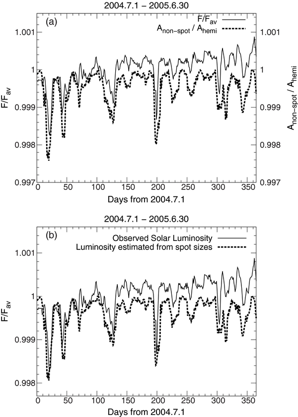
Figure 8. (a) Normalized irradiance of the Sun and the area not covered by sunspots. The data period is 2004 July 1–2005 June 30. The solid lines are normalized visible (4500–8000 Å) solar irradiance from the solar spectral irradiance data of the SORCE satellite. We use the daily sunspot area data prepared by the US Department of Commerce, NOAA, and the Space Weather Prediction Center. (b) Normalized irradiance of the Sun and the luminosity estimated from the spot coverages assuming that the temperature of sunspots is 4000 K and that of the solar photosphere is 6000 K. The data period is the same as in (a).
Download figure:
Standard image High-resolution imageIn the following, we discuss the relationship between the starspot coverage and the superflare energy. Flares are the release of stellar magnetic energy (e.g., Shibata & Magara 2011). It is known that there are positive correlations between the sunspot coverage and the energy of the largest solar flares (Sammis et al. 2000). It is, therefore, important to consider whether the same correlations can be found and the observed maximum superflare energy can be explained by the magnetic energy of large starspots that many superflare stars are expected to have. Although we have already simply discussed the relationship between the amplitude of superflares and that of the brightness variations in the Supplementary Information section of Maehara et al. (2012), here we advance this former analysis and discuss whether the magnetic energy of starspots can explain the energy of the superflares by applying the results from this paper, i.e., that starspot coverages can be roughly estimated from the brightness variation.
First, we discuss the expected relationships if the energy sources of the superflares are the magnetic energy stored around the starspots (Eflare ⩽ Emag). The total energy released by the flare must be smaller than (or equal to) the magnetic energy stored around the starspots. The order of the stored magnetic energy (Emag) can be roughly estimated by

where B and l correspond to the magnetic field strength and the size of the starspot region. It should be noted that we cannot exclude the possibility that starspots of superflare-generating stars are collections of smaller spots.
We roughly assume that there is a linear correlation between the brightness variation and the spot coverage when we estimate the magnetic energy stored around the starspots based on the amplitude of the brightness variation. The total amplitude of the brightness variation due to the rotation normalized by the average brightness (ΔFrot) can be expressed by

where Aspot is the total area of the starspots and Aphot is the total visible area of the stellar surface. Since the Kepler photometer covers a wide spectral range (4000–8500 Å), observed brightness changes would be nearly approximated by the bolometric brightness change obtained by Equation (8).
If we assume that  , Equation (7) can be transformed to

where Eflare is the total energy released by the flare. The amplitude of the flare normalized by the average brightness (ΔFflare) can be estimated by

where Lstar is the luminosity of the star and τ is the e-folding time of the flare. Then the relationship between the flare amplitude and the brightness variation amplitude can be written as
This indicates that the upper limit of the flare amplitude is proportional to 1.5 power of the starspot area if we assume B = constant. We discuss below whether this assumption is right.
The discussion around Equations (7)–(11) does not take into account the effect of the inclination angle i and the spot latitude. In stars with a lower inclination angle and higher spot latitude, the amplitude of the brightness variation is smaller. If we consider inclination effects and assume that the spot is near the equator, Equation (11) can be replaced by Equation (12):
If we adopt Lstar = 1033 erg s−1, τ = 104 s, Tspot = 4000 K, and Tphot = 6000 K for superflares on solar-type stars, then the flare amplitude can be roughly estimated by
Figure 9 is the scatter plot of the superflare amplitude as a function of the brightness variation amplitude. The superflare data are taken from Quarters 1–6 data and are reported in Shibayama et al. (2013). The lines in this figure represent the analytic relation between the flare amplitude and the amplitude of the brightness variation obtained from Equation (13) for i = 90° and i = 2° (nearly pole-on). Taking into account that the magnetic energy density of solar-type stars is about 1000–4000 G (Solanki 2003), we show two lines (B = 1000 G and 3000 G) for each inclination angle. These lines give an upper limit for the flare amplitude based on the above discussion. Many of the flares have smaller amplitudes than predicted by Equation (13). Moreover, all flares have smaller flare amplitudes than expected in the nearly pole-on case (dashed line; i = 2°). This supports the idea that the energy released by these flares can be explained by the magnetic energy stored near the starspots.

Figure 9. Scatter plot of the superflare amplitude as a function of the amplitude of the brightness variation. The data for the superflares are taken from Quarters 1–6 data and are reported in Shibayama et al. (2013). Here we define the amplitude as the normalized brightness range, in which the lower 99% of the distribution of the brightness difference from average, except for the flares, are included. The thick and thin solid lines correspond to the analytic relationship between the stellar brightness variation amplitude (corresponding to the spot area) and flare amplitude (corresponding to the flare energy) obtained from Equation (13) for B = 3000 G and 1000 G, respectively. The thick and thin dashed lines correspond to the same relationship for i = 20 (nearly pole-on) for B = 3000 G and 1000 G. These lines are considered to give an upper limit for the flare amplitude.
Download figure:
Standard image High-resolution imageFor the solar flares, there is a similar relationship to the one discussed above (Sammis et al. 2000). Figure 10 shows the empirical relationship between the spot group area and the X-ray intensity of solar flares (Sammis et al. 2000), and the relationship between the spot group area (estimated from the brightness variation amplitude) and the superflare energy. It should be noted that while there is a large range in observed flare energies for a given sunspot area, here we refer to the upper envelope of the observations shown in Figure 10, where the largest flare energies are associated with larger spots. The bolometric luminosity and the total bolometric energy of the superflares were estimated from the stellar radius, the effective temperature in the Kepler Input Catalog (Brown et al. 2011), and the observed amplitude and duration of the flares by assuming that the spectrum of white light flares can be described by blackbody radiation with an effective temperature of ∼10,000 K (Kretzschmar 2011). Using concrete numerical values, Equation (9) is transformed as
where R☉ is the radius of the Sun. The relationship expressed by Equation (14) can be seen in Figure 10. All of the solar flare data and over half of the superflare data are located below the line B = 1000 G and i = 90°.

Figure 10. Flare energy vs. spot coverage of superflares on solar-type stars (filled squares; Shibayama et al. 2013) and solar flares (filled circles; Sammis et al. 2000; T. T. Ishii 2012, private communication). The solar flare data of are taken from ftp://ftp.ngdc.noaa.gov/STP and consist of data taken in 1989–1997 (Sammis et al. 2000) and in 1996–2006 (T. T. Ishii 2012, private communication). The thick and thin solid lines correspond to the analytic relationship between the flare energy obtained from Equation (14) for B = 3000 G and 1000 G, respectively. The thick and thin dashed lines correspond to the same relationship for i = 20 (nearly pole-on) B = 3000 G and 1000 G. These lines are considered to give an upper limit for the flare energy (i.e., the maximum possible magnetic energy that can be stored near sunspots). Note that the superflares on solar-type stars are observed only with visible light and the total energy is estimated from the visible light data. Hence, the X-ray intensity in the right-hand vertical axis is not based on actual observations. The energy of solar flares is based on the assumption that the energy of the X10-class flare is 1032 erg, X-class is 1031 erg, M-class is 1030 erg, and C-class is 1029 erg, considering previous observational estimates of the energy of typical solar flares (e.g., Benz 2010). The values on the top horizontal axis show the total magnetic flux of the spot corresponding to the area on the horizontal axis at the bottom when B = 1000 G.
Download figure:
Standard image High-resolution image
Figure 11.
Light curves of solar-type superflare stars from Kepler Quarter 0–6 data. (The complete figure set (238 images) is available in the online journal)
Download figure:
Standard image High-resolution imageSome superflare data points are located above the Equation (14) line. This is explained by two reasons. First, the inclination and latitude of the spots govern their projected area, and the size of the spot cannot be uniquely determined because of this effect and the fixed contrast with the photosphere. Lower inclinations cause a smaller projected spot area and/or the spot to be visible through most of the rotation period, and therefore lower brightness variations result in these cases.
Second, the magnetic flux density (B) is not necessarily constant. It is a function of the spot size. Solanki (2003) shows that the umbral continuum intensity of sunspots becomes weak as sunspots become large and the magnetic flux density becomes strong. This means that as the spot becomes larger, the magnetic flux density becomes stronger and the magnetic energy stored near the spot increases. As a result, the released flare energy tends to be bigger than that in the case of B = constant, and the lines in Figure 10 become steeper.
In this paper, we show that many superflare-generating stars probably have large starspots, and that the energy of the superflares can be explained by the magnetic energy stored around such starspots. We also confirmed in Section 4 that the stellar activity depends on the rotation period. Stars with relatively slower rotation rates can still produce flares that are as energetic as those of more rapidly rotating stars, but their average flare frequency is lower. There are, however, many things to consider in the next step. For example, it is extremely important to know the lifetime of starspot regions and how the activity level changes, because it is related to determining how the starspot evolves by the dynamo mechanism. Shibata et al. (2013) indicated that the magnetic energy required to generate superflares can be produced by the effects of differential rotation. We need to investigate in detail the effects of differential rotation on the brightness variation.
If superflares occur on the starspot area of a single star and the brightness variation is caused by the rotation, then their timing is likely to have a phase dependence, since superflares that we can observe need to occur when the starspots are on the visible side of the star. This phase dependence, however, is expected not to be necessarily true. For some pairs of spot distribution on the stellar surface and stellar inclination angle, part of the area covered by the starspots is always on the visible side of the star. In these cases, it is probable that superflares occur in any phase of the differential rotation. We need to study these effects in detail in the next step (cf. Roettenbacher et al. 2013 discuss these effects for one K-type star).
6. SUMMARY
In this paper, we investigated the brightness variations of superflare-generating stars in Kepler Quarters 0–6 data by considering the signature of stellar rotation and the starspots. First, we performed simple spot-model analyses for typical superflare-generating stars. Many of the brightness variations with a period of one day to a few tens of days and an amplitude of 0.1%–10% can be explained by the star's rotation and the presence of fairly large starspots, taking into account the effects of the inclination angle and the spot latitude. Next, using the results of the period analysis, we investigated the relationship between the energy and frequency of superflares and the rotation period by assuming that the period of the brightness variation corresponds to the rotation period. Stars with relatively slower rotation rates can still produce flares that are as energetic as those of more rapidly rotating stars, although the average flare frequency is lower for more slowly rotating stars. Last, we discussed the relationship between the starspot coverage and the energy of flares. If we assume that the brightness variations are due to the rotation, the energy of superflares can be explained by the magnetic energy stored near the large starspots.
We are grateful to Professor Kazuhiro Sekiguchi (NAOJ) for providing useful suggestions. We also thank the anonymous referee for the helpful comments. Kepler was selected as the 10th Discovery Mission. Funding for this mission is provided by the NASA Science Mission Directorate. The data presented in this paper were obtained from the Multimission Archive at STScI. This work was supported by the Grant-in-Aid from the Ministry of Education, Culture, Sports, Science, and Technology of Japan (No. 25287039).
Footnotes
- 5
- 6
For the detrend method used by the Kepler pipeline, see http://keplergo.arc.nasa.gov/PyKEprimerCBVs.shtml.