


ABSTRACT
We report new measurements of the elemental energy spectra and composition of galactic cosmic rays during the 2009–2010 solar minimum period using observations from the Cosmic Ray Isotope Spectrometer (CRIS) onboard the Advanced Composition Explorer. This period of time exhibited record-setting cosmic-ray intensities and very low levels of solar activity. Results are given for particles with nuclear charge 5 ⩽ Z ⩽ 28 in the energy range ∼50–550 MeV nucleon−1. Several recent improvements have been made to the earlier CRIS data analysis, and therefore updates of our previous observations for the 1997–1998 solar minimum and 2001–2003 solar maximum are also given here. For most species, the reported intensities changed by less than ∼7%, and the relative abundances changed by less than ∼4%. Compared with the 1997–1998 solar minimum relative abundances, the 2009–2010 abundances differ by less than 2σ, with a trend of fewer secondary species observed in the more recent time period. The new 2009–2010 data are also compared with results of a simple "leaky-box" galactic transport model combined with a spherically symmetric solar modulation model. We demonstrate that this model is able to give reasonable fits to the energy spectra and the secondary-to-primary ratios B/C and (Sc+Ti+V)/Fe. These results are also shown to be comparable to a GALPROP numerical model that includes the effects of diffusive reacceleration in the interstellar medium.
Export citation and abstract BibTeX RIS
1. INTRODUCTION
In the heliosphere, the interstellar composition and energy spectra of the inwardly diffusing galactic cosmic ray (GCR) nuclei are distorted by interactions with the magnetic field being convected outward by the expanding solar wind, a process referred to as "solar modulation." Nuclei with interstellar energies less than a few GeV nucleon−1 lose a significant fraction of their energy due to adiabatic deceleration. These losses vary with the changing ∼11 yr solar cycle and are smallest during the solar-minimum phase of the cycle.
The most recent solar minimum, occurring in 2007–2010, exhibited very low levels of solar activity and the highest measured GCR intensities of the space era (Mewaldt et al. 2010). Observations during this time are the closest we have come in the inner solar system to observing GCR nuclei in interstellar medium (ISM) conditions. Model calculations (see Section 6) suggest that the intensities of GCR nuclei with 5 ⩽ Z ⩽ 28 were 40%–65% of local interstellar values for all energies above 160 MeV nucleon−1, the energy at which CRIS is sensitive to all of these species (Section 5). At higher energies, the spread becomes smaller and the ratio of the 1 AU intensities to the local ISM intensities approaches unity. With these data we can shed light on interstellar transport processes, and ultimately determine better estimates for the GCR source composition.
The Advanced Composition Explorer (ACE; Stone et al. 1998b) was launched on 1997 August 25 and is located in a halo orbit about the L1 Lagrangian point 1.5 million kilometers sunward from Earth. It carries nine instruments designed to study the solar wind, the solar magnetic field, solar energetic particles (SEPs), anomalous cosmic rays, and GCRs. The Cosmic Ray Isotope Spectrometer (CRIS; Stone et al. 1998a) measures the charge, mass, and energy of GCRs with nuclear charge 3 ⩽ Z ⩽ 30 in the energy range ∼50–550 MeV nucleon−1. With its large geometrical acceptance of ∼250 cm2 sr and its excellent charge and mass resolution, CRIS provides the most detailed records of GCR composition to date.
The scope of this paper is two-fold. In the first part we report CRIS measurements of the elemental composition and energy spectra for GCR nuclei with 5 ⩽ Z ⩽ 28 during the most recent solar minimum period. In the second part we discuss improvements to our simple leaky-box interstellar transport model and compare our new model results with GALPROP models (Strong & Moskalenko 1998) incorporating both simple diffusion and diffusion plus diffusive reacceleration.
2. INSTRUMENT DESCRIPTION
The CRIS instrument consists of four stacks of silicon solid-state detectors (SSDs) positioned below a scintillating optical fiber trajectory (SOFT) hodoscope (see Figure 1). The silicon stacks, which each contain 15 circular SSDs grouped into 9 detectors, are used to measure the energy losses of charged particles. The square SOFT hodoscope is used to determine the trajectories of incident particles using three x–y tracking layers. The fibers in each plane are coupled to the face of an image intensifier, which is then coupled to a 244 × 550 pixel charge-coupled device (CCD). There are two image intensifier/CCD camera systems, though only one of the two cameras has been used for data readout. An additional x–y pair at the top of the instrument serves as the trigger layer. The charge, mass, and incident energy at the top of the instrument for cosmic rays stopping in the silicon stacks are determined from the energy deposited in the detector in which the particle stopped (E', in MeV) and multiple measurements of the rate of energy loss in the other detectors through which it passed (dE/dx, in MeV g−1 cm2). A detailed description of the CRIS instrument is found in Stone et al. (1998a).
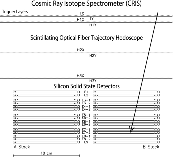
Figure 1. CRIS instrument cross section (two of four circular silicon detector stacks shown). Particle trajectories are determined using three x–y layers of scintillating optical fibers, with a fourth layer serving as the trigger. The arrow shown represents the trajectory of a particle stopping in the bottom wafer of detector E7.
Download figure:
Standard image High-resolution image3. DATA SELECTION
CRIS data presented here include all species from boron (Z = 5) to nickel (Z = 28) stopping in detectors E2–E8. Data for the recent solar minimum period were obtained from 2009 March 23 to 2010 January 13, a 297 day period characterized by record-setting cosmic-ray intensities (Mewaldt et al. 2010). During this period there were no large SEP events and the average live time for the CRIS instrument was ∼79%, for a total of ∼235 days of data; the dead time is due to instrument activities such as event processing, pulser calibrations, leakage current balancing, etc. (Stone et al. 1998a). The variation of the GCR intensity over the life of CRIS is seen in Figure 2, which shows the oxygen intensity (solid line) in the energy band 77.2–103.8 MeV nucleon−1 as a function of time. For reference the observed sunspot numbers (dotted line) from the Royal Observatory of Belgium are also shown (http://sidc.oma.be).
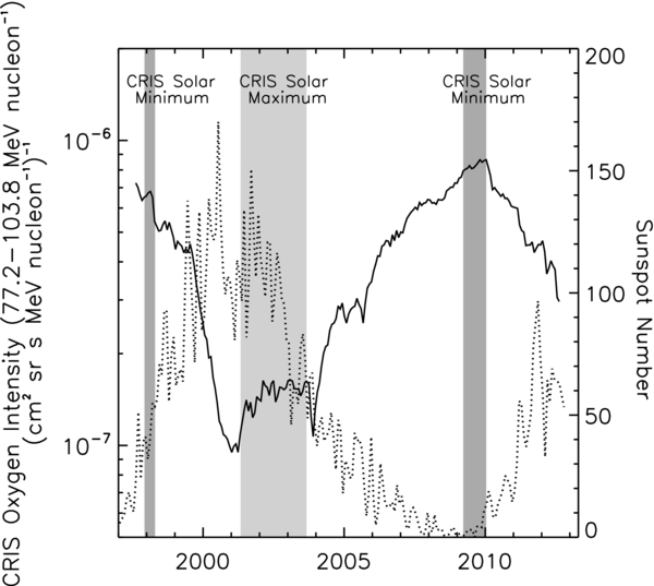
Figure 2. CRIS oxygen intensity (solid line), averaged over the 27 day Bartels rotation, for the mission to date. The shaded regions indicate the dates of the solar minimum (darker gray) and maximum (lighter gray) periods analyzed in this work. For reference, the observed sunspot numbers (dotted line) from the Royal Observatory of Belgium (http://sidc.oma.be) are also shown.
Download figure:
Standard image High-resolution imageGeorge et al. (2009) presented data for the 1997–1998 solar minimum (1997 August 28 to 1998 April 20) and the 2001–2003 solar maximum (2001 May 1 to 2003 September 1) periods. Since that publication, small corrections have been made to the data analysis, including a change in the period of time analyzed for the 1997–1998 solar minimum. Appendix A.1 discusses the changes and the revised data are given in Tables 1, 4, 5, 7, and 8. For most species, the reported intensities changed by less than ∼7%, while the relative abundances changed by less than ∼4%.
Table 1. CRIS Relative Elemental Abundances at 160 MeV nucleon−1
| Element | 1997–1998 | 2001–2003 | 2009–2010 |
|---|---|---|---|
| B | 1788.6 ± 30.1 | 1996.8 ± 24.9 | 1725.7 ± 19.4 |
| C | 7227.0 ± 73.3 | 6712.6 ± 51.9 | 7235.4 ± 45.0 |
| N | 1705.2 ± 20.9 | 1826.4 ± 16.9 | 1678.9 ± 12.3 |
| O | 7067.2 ± 70.9 | 6535.8 ± 50.1 | 7137.0 ± 42.7 |
| F | 99.4 ± 3.5 | 124.1 ± 3.1 | 97.3 ± 2.1 |
| Ne | 1005.5 ± 14.1 | 1053.4 ± 11.2 | 998.9 ± 8.4 |
| Na | 190.3 ± 4.9 | 212.1 ± 4.0 | 185.2 ± 2.9 |
| Mg | 1374.3 ± 17.3 | 1370.9 ± 13.1 | 1375.3 ± 10.3 |
| Al | 199.4 ± 4.7 | 226.1 ± 3.9 | 203.2 ± 2.8 |
| Si | 1000.0 ± 13.0 | 1000.0 ± 9.8 | 1000.0 ± 7.8 |
| P | 26.7 ± 1.5 | 34.4 ± 1.3 | 26.7 ± 0.9 |
| S | 155.7 ± 3.7 | 179.8 ± 3.0 | 157.0 ± 2.2 |
| Cl | 26.0 ± 1.7 | 37.5 ± 1.6 | 24.8 ± 0.8 |
| Ar | 58.4 ± 2.1 | 78.0 ± 1.9 | 55.3 ± 1.2 |
| K | 39.9 ± 1.7 | 62.2 ± 1.7 | 40.1 ± 1.0 |
| Ca | 126.5 ± 3.3 | 156.5 ± 2.9 | 119.5 ± 1.9 |
| Sc | 26.4 ± 1.1 | 34.1 ± 1.0 | 25.3 ± 0.9 |
| Ti | 102.3 ± 3.1 | 124.7 ± 2.6 | 100.5 ± 1.8 |
| V | 46.0 ± 2.1 | 54.7 ± 1.8 | 48.1 ± 1.3 |
| Cr | 100.2 ± 3.3 | 110.4 ± 2.7 | 98.8 ± 1.9 |
| Mn | 63.3 ± 2.7 | 70.0 ± 2.2 | 61.9 ± 1.6 |
| Fe | 673.7 ± 10.9 | 737.1 ± 8.9 | 671.4 ± 6.5 |
| Co | 4.4 ± 0.3 | 4.6 ± 0.3 | 3.7 ± 0.4 |
| Ni | 31.6 ± 2.2 | 33.8 ± 1.8 | 29.9 ± 1.3 |
Notes. Values are normalized to Si≡1000. Only the statistical uncertainties are given. The absolute intensity (with combined statistical and systematic uncertainties) for silicon at 160 MeV nucleon−1 is (108.2 ± 3.4) × 10−9 (cm2 s sr MeV nucleon−1)−1 for the 1997–1998 solar minimum, (29.4 ± 0.9) × 10−9 (cm2 s sr MeV nucleon−1)−1 for the 2001–2003 solar maximum, and (132.5 ± 4.1) × 10−9 (cm2 s sr MeV nucleon−1)−1 for the 2009–2010 solar minimum.
Download table as: ASCIITypeset image
The data used for this paper have been selected using several criteria. These include geometrical cuts to ensure particles passed within the active areas of each detector, charge consistency cuts to eliminate interactions in the instrument, and checks on the quality of the calculated trajectories. For further information regarding these selection criteria, refer to George et al. (2009).
4. ELEMENTAL SPECTRA
Elemental intensities in seven energy bins, corresponding to cosmic rays stopping in each of the detectors E2–E8, for the 2009–2010 solar minimum are given in Appendix B in Table 6. These data are plotted in Figure 3, where we have applied arbitrary energy-independent scale factors to allow for easy comparison of the shapes of the spectra. These spectra were corrected for the geometrical acceptance, energy intervals, the detection efficiency of the hodoscope, fragmentation in the instrument, and the livetime (for further details on the calculation, refer to Appendix A).
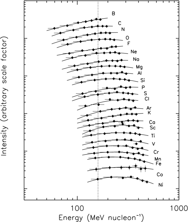
Figure 3. CRIS elemental GCR spectra during the 2009–2010 solar minimum (refer to Table 6). Arbitrary energy-independent scale factors have been applied to the intensity of each element for the comparison of the spectral shapes. The solid lines are quadratic fits to the data used to determine the relative abundances. The dotted line at 160 MeV nucleon−1 indicates the energy at which these abundances are reported (Table 1).
Download figure:
Standard image High-resolution imageThe statistical uncertainties for the intensities in individual energy bins are typically small for all but the rarest species, varying from 0.4% for oxygen up to ∼7% for phosphorus, chlorine, and scandium. Cobalt is the rarest species reported here, with statistical uncertainties up to ∼18%. Systematic uncertainties are a combination of the uncertainties on the geometrical acceptance (2%), the hodoscope efficiency (2%), and the fragmentation correction (range- and charge-dependent: 0.5% for boron up to 1.1% for nickel stopping in E2, and 3.4% for boron up to 8.9% for nickel stopping in E8). The total uncertainties quoted in Tables 4, 5, and 6 are the quadratic sum of the statistical and systematic contributions.
5. COMPOSITION
In Figure 3, the vertical dotted line at 160 MeV nucleon−1 denotes the energy at which the relative elemental abundances are taken. The GCR composition is energy-dependent, and at this energy the CRIS instrument is sensitive to all of the species considered in this work. To determine the relative abundances we fit parabolas in log(Intensity) versus log(Energy/nucleon) to the seven energy bins for each element. These fits are shown as solid lines in Figure 3. Relative abundances are calculated from the ratios of these fits at 160 MeV nucleon−1. These abundances, normalized to Si≡1000, are given in Table 1, where updated abundances for the 1997–1998 solar minimum and the 2001–2003 solar maximum are also shown. Only statistical uncertainties are quoted in this table, since the residual systematic uncertainties tend to cancel out when comparing the abundance ratios of nearby species.
Figure 4 compares the relative abundances for the different time periods. In the bottom panel are the ratios of the 1997–1998 solar minimum abundances relative to the 2009–2010 abundances given in Table 1. We see that there is good agreement between the two solar minimum periods. The differences between the relative abundances are less than 2σ for all species, with the largest differences (1.8σ) for both boron (Z = 5) and calcium (Z = 20).
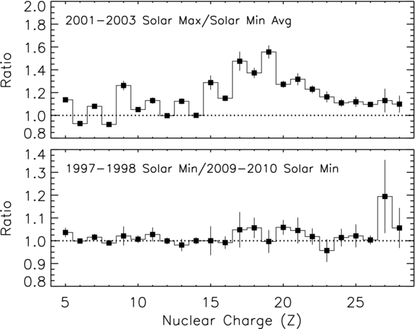
Figure 4. Ratios of the CRIS relative abundances given in Table 1. The top panel plots the 2001–2003 solar maximum abundances relative to the average (unweighted arithmetic mean) solar minimum abundances. The bottom panel plots the 1997–1998 solar minimum abundances relative to the 2009–2010 abundances.
Download figure:
Standard image High-resolution imageThe 2001–2003 solar maximum relative abundances are also compared with the average (unweighted arithmetic mean) solar minimum abundances, as shown in the top panel of Figure 4. During periods of greater solar modulation, arriving GCRs lose more energy in the heliosphere; therefore, on average, the GCRs come from higher energy particles outside the heliosphere (Niebur et al. 2003). At CRIS energies the higher energy solar maximum particles have traversed longer path lengths in the Galaxy, implying the production of more secondary species, as is clearly seen in Figure 4. Further discussion on this observation is found in George et al. (2009).
The same effect is seen at a lower level of significance in the bottom panel of Figure 4. Here the denominator of the plotted ratio is from a period with slightly lower solar modulation than the numerator, resulting in higher ratios for most secondaries than for primaries.
6. DISCUSSION
6.1. Simple Leaky-box Transport Model
The transport of cosmic rays from their galactic sources to Earth is modeled in two steps: the interstellar transport and the solar modulation (discussed in Section 6.2). Beginning with a set of assumed source abundances (refer to George et al. 2009) and an injection spectrum that is a power law in momentum with a spectral index of −2.35, we determine the equilibrium interstellar intensities φi as a function of energy per nucleon ε using a steady-state leaky-box transport model based on the formalism of Meneguzzi et al. (1971):
The terms on the left-hand side of this equation represent the production of species i given the source (qi), nuclear spallation, radioactive decay, and changes to the ionic charge state (the attachment or stripping of an orbital electron). These contributions are written in terms of the corresponding mean free paths ( ,
,  , and
, and  , respectively). The summation is over all species j capable of producing species i. The right-hand side of Equation (1) contains terms representing the losses of species i due to nuclear spallation, radioactive decay, ionic charge state changes, and escape from the Galaxy. Again, these contributions are written in terms of the mean free paths (
 ,
,  ,
,  , and
, and  , respectively). The final term on the right-hand side of the equation accounts for spectral changes due to ionization energy loss, with wi ≡ (dε/dx)i representing the specific ionization per nucleon in the ISM. We do not include spectral changes due to reacceleration processes in the ISM. Studies by Heinbach & Simon (1995) and Scott (2005) have shown that the effects of reacceleration are relatively minor at the interstellar energies of the GCRs observed by CRIS. This transport model is described in further detail in Lave (2012), which presents a number of updates to the model used in George et al. (2009). These changes are also summarized below.
The most important change to the interstellar transport model involved an extensive revision of our database of high-energy production cross section measurements and the semi-empirical cross section formulae used to account for nuclear spallation in the ISM. We used the database maintained by the National Nuclear Data Center (NNDC, http://www.nndc.bnl.gov/nudat2/) to update our compilation of cross sections for reactions of parent nuclei with charge Z ⩽ 28 interacting on hydrogen at energies between ∼300–1500 MeV nucleon−1 that produce daughter nuclei from 7Be through 57Ni. For a full listing of the cross section references and a complete description of their usage in our transport code, refer to Lave (2012). The semi-empirical cross section formulae of Silberberg et al. (1998) and Tsao et al. (1998) based on the yieldx_080999.for version of their code have been updated with the help of A. F. Barghouty (2010, private communication; hereafter referred to as S&T).
For all reactions with available measurements, we compared the S&T cross sections with the data and calculated energy-independent scale factors for S&T that would yield the best agreement. For most reactions, the rescaled S&T cross sections agreed quite well with the data. A few reactions exhibited significant discrepancies with the data, and these reactions were studied on an individual basis to determine the parameterization that best fit the available cross section measurements (Lave 2012).
Another important change to our transport model involved the parameterization of the mean free path for escape in the Galaxy (Λesc). The previous work of George et al. (2009) used the form given by Davis et al. (2000):
where β is the ratio of the particle velocity to the speed of light, R is the particle rigidity (in GV), and the coefficients C0–C4 are given in Table 2. This form was based on the work of Soutoul & Ptuskin (1999), which assumed a galactic wind that convects GCRs from the Galaxy with a velocity that is a non-monotonic function of the distance from the galactic plane. In updating our interstellar transport model, we retained the functional form used in Davis et al. (2000) and again in George et al. (2009) but adjusted its parameters to obtain the best fit using the data that are now available.
Table 2. Fit Coefficients for the Escape Mean Free Path Parameterization
| Model | C0 | C1 | C2 | C3 | C4 |
|---|---|---|---|---|---|
| (GV) | (GV) | ||||
| George et al. (2009) | 29.50 | 1.00 | 0.60 | 1.30 | −2.00 |
| This work | 32.45 | 0.90 | 0.59 | 1.17 | −1.60 |
Download table as: ASCIITypeset image
Using the new solar minima energy spectra presented in this work, we have adjusted the values of C0–C4 by minimizing the reduced χ2 values for the fits of the transport model results to the measured B/C and (Sc+Ti+V)/Fe ratios (Section 6.3.2). The new coefficients are listed in Table 2, and the two parameterizations are compared in Figure 5.
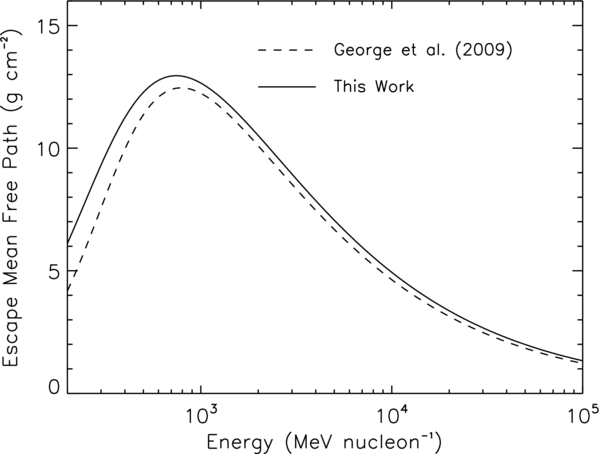
Figure 5. The escape mean free path parameterizations for a particle with a mass-to-charge ratio of 2, calculated using Equation (2) and the coefficients given in Table 2. The solid line uses the new parameterization presented in this work, while the dashed line uses the parameterization from George et al. (2009).
Download figure:
Standard image High-resolution image6.2. Solar Modulation Model
Following the derivation of the equilibrium interstellar spectra, the effects of solar modulation are calculated taking into account diffusion, convection, and adiabatic deceleration using the spherically-symmetric Fokker–Planck equation (Goldstein et al. 1970). This equation is solved using the Crank–Nicholson technique discussed by Fisk (1971). This allows for the calculation of GCR intensities anywhere in the heliosphere given the interstellar intensities and values for the outer radius D of the modulation region, the solar wind velocity VSW(r) as a function of radius, and the diffusion coefficient κ(r, R) as a function of radius and particle rigidity R.
We make the simplifying assumptions that VSW and κ are independent of radius and that κ has the form κ(R) = κ0βR/R0, where κ0 is the value of the diffusion coefficient at a reference rigidity R0 and β is the particle velocity relative to the speed of light. If one assumes values for VSW and D, the modulation is fully specified by a single parameter, κ0. The forms adopted for VSW and κ correspond to the conditions assumed by Gleeson & Axford (1968) in deriving the approximate "force-field" solution to the modulation equation. That approximation is characterized by a "modulation potential" ϕ (measured in MV) that is related to D, VSW, and κ by the equation
Thus there is a one-to-one correspondence between ϕ and κ0, and although we use the full solution of the modulation equation and not the force-field approximation, ϕ still provides a convenient parameter for characterizing the level of solar modulation.
We determined the modulation potential for a given time period by comparing the CRIS energy spectra for each 27 day solar rotation to model spectra templates calculated for a variety of ϕ values (Wiedenbeck et al. 2005). Figure 6 shows the time dependence of ϕ derived from the primary species carbon, silicon, and iron. For solar minimum periods, ϕ values for the different species typically agree to within 25–50 MV; for solar maximum periods, the agreement between the species is within ∼100 MV. Due to the simplifications in our solar modulation model, individual species are not necessarily best fit with the same modulation parameter. Therefore, we have chosen to adopt average modulation levels for each time period studied here. In the Fisk model, we used values of κ0 corresponding to the following values of ϕ: 250 MV (2009–2010 solar minimum), 325 MV (1997–1998 solar minimum), and 900 MV (2001–2003 solar maximum).
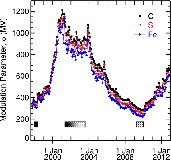
Figure 6. Time dependence of the modulation potential ϕ for select primary species. These curves were obtained by comparing model spectra templates to the CRIS energy spectra for each 27 day solar rotation. The horizontal bars at the bottom of the figure indicate the time periods for the 1997–1998 solar minimum (solid bar), the 2001–2003 solar maximum (cross-hatched bar), and the 2009–2010 solar minimum (forward-hatched bar).
Download figure:
Standard image High-resolution image6.3. Testing the Transport Model
Interstellar transport models are commonly tested by examining the ratios B/C and (Sc+Ti+V)/Fe (Section 6.3.2) because they probe the mean amount of material that cosmic rays traverse before escaping from the Galaxy, and they are less sensitive to the injection spectrum and the solar modulation model than the energy spectra. The species in the numerators of these ratios are very rare in solar system material and are almost entirely secondary nuclei produced from the fragmentation of the nearly pure primary species in the denominators.
6.3.1. Select Element Spectra
Figures 7 and 8 show the energy spectra for the 2009–2010 solar minimum period for boron, carbon, scandium, titanium, vanadium, and iron. Also plotted in these figures are data from various other experiments that cover energies between ∼10–105 MeV nucleon−1. The solid lines give our calculated spectra corresponding to ϕ = 250 MV, while the shaded regions indicate the range of model results for ±25 MV variations about this value. We note that the relative differences in the widths of the shaded regions for various elements are the result of the differences in the interstellar spectra. In the ISM, primary species such as carbon and iron peak at lower interstellar energies than the secondary species, which affects the modulated spectra at low energies. Also shown is our model calculation for a modulation value of 750 MV (dotted lines), which is appropriate for the HEAO-3 data.
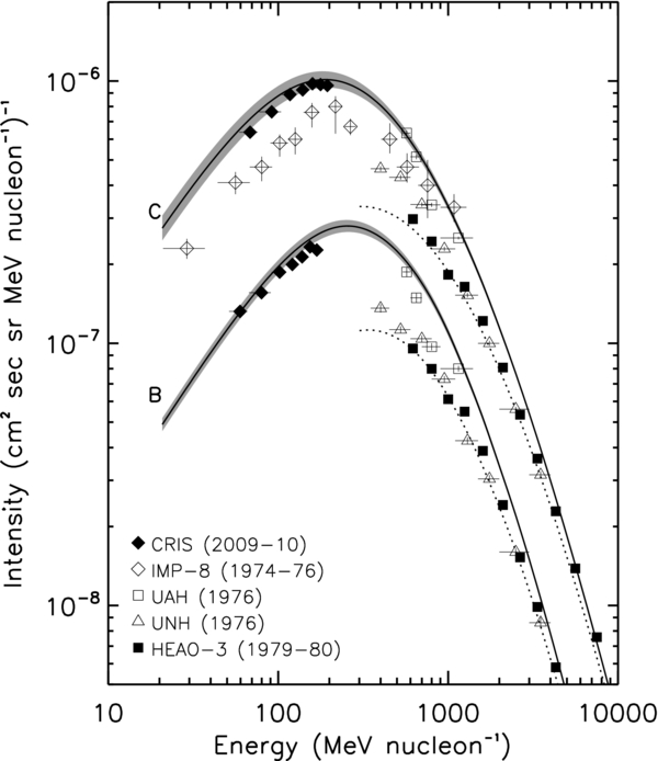
Figure 7. Observed spectra for boron and carbon, including the CRIS 2009–2010 solar minimum data. Other experimental data include two space missions, IMP-8 (Garcia-Munoz et al. 1977) and HEAO-3 (Engelmann et al. 1990), as well as two balloon-based experiments, the University of Alabama, Huntsville (UAH; Derrickson et al. 1992) and the University of New Hampshire (UNH; Lezniak & Webber 1978). The solid curves are the results from our transport model corresponding to a modulation value of 250 MV, with the shaded regions indicating the model results for a ±25 MV variation about this value. The dotted curves give the results corresponding to ϕ = 750 MV.
Download figure:
Standard image High-resolution image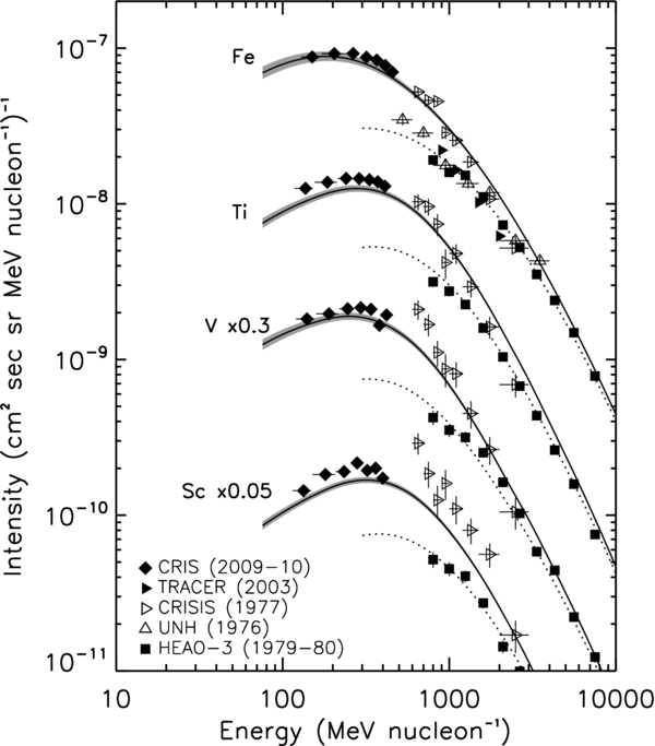
Figure 8. Observed spectra for scandium, titanium, vanadium, and iron, including the CRIS 2009-10 solar minimum data. In addition to the experimental data referenced in Figure 7, we have added data from two additional balloon-based experiments: TRACER (Ave et al. 2008) and CRISIS (Young et al. 1981). The solid curves are the results from our transport model corresponding to ϕ = 250 MV, with the shaded regions indicating the model results for a ±25 MV variation about this value. The dotted curves correspond to ϕ = 750 MV.
Download figure:
Standard image High-resolution imageThe CRIS boron, carbon, and iron spectra are fairly well fit by the model with typical differences of ∼6%–8%. The scandium, titanium, and vanadium spectra are less well-fit by the model, with differences of ∼9%–15%. These differences are not surprising since Figure 6 indicates that carbon and iron are better fit with models corresponding to slightly higher and lower values of ϕ, respectively. These results illustrate the difficulty in simultaneously fitting the energy spectra of all species using our simplified solar modulation model (as was previously discussed in Section 6.2). More sophisticated models have been studied (see Potgieter 2011 for a review), though we have not attempted to do so here.
Since the other experiments operated during different periods of time in the solar cycle, we do not expect these data to be fit using the same modulation value. Therefore we have used the procedure described in George et al. (2009) to normalize all of the data to the same modulation level as the CRIS data, as shown in Figures 9 and 10. Here we have used models that correspond to the following values of ϕ: 275 MV (CRISIS), 325 MV (UAH), 400 MV (IMP-8), 625 MV (UNH), and 900 MV (TRACER). With the exception of the CRISIS data, which have large uncertainties for the rarer sub-iron species, we see that these data are all reasonably well fit by the model.
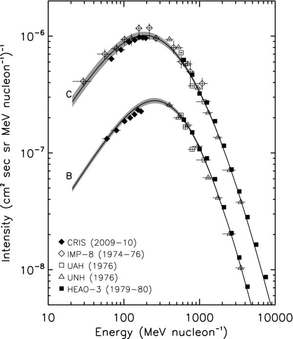
Figure 9. Observed spectra for boron and carbon, including the CRIS 2009–2010 solar minimum data. This figure is the same as Figure 7, except the other experimental data have been adjusted to the CRIS modulation level of ϕ = 250 MV according to the procedure described in George et al. (2009). The shaded regions indicate the model results for a ±25 MV variation about this value of ϕ.
Download figure:
Standard image High-resolution image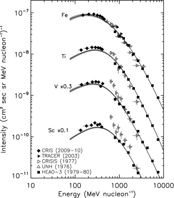
Figure 10. Observed spectra for scandium, titanium, vanadium, and iron, including the CRIS 2009-10 solar minimum data. This figure is the same as Figure 8, except the other experimental data have been adjusted to the CRIS modulation level of ϕ = 250 MV according to the procedure described in George et al. (2009). The shaded regions indicate the model results for a ±25 MV variation about this value of ϕ.
Download figure:
Standard image High-resolution image6.3.2. Secondary-To-Primary Ratios
Figure 11 shows the B/C and (Sc+Ti+V)/Fe ratios from CRIS for the 2009–2010 solar minimum. Measurements from additional experiments are plotted above 400 MeV nucleon−1: HEAO-3, TRACER (Obermeier et al. 2011), CRN (Swordy et al. 1990), ATIC-2 (Panov et al. 2008), AMS-01 (Aguilar et al. 2010), and CREAM (Ahn et al. 2008). Data are plotted using statistical uncertainties; the exceptions to this are the data from CRN and ATIC, which only reported total uncertainties. The solid lines give the ratios calculated from our transport model corresponding to a modulation value of 250 MV, with the shaded regions indicating the range of results for a ±25 MV variation of this value.
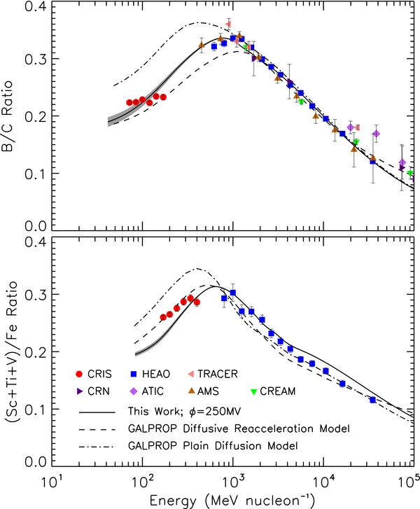
Figure 11. CRIS B/C and (Sc+Ti+V)/Fe ratios for the 2009–2010 solar minimum period (circles). Data from additional experiments (see Section 6.3.2 for the references) are plotted above 400 MeV nucleon−1. The solid curves are the result of our transport model corresponding to a modulation value of 250 MV, with the shaded regions indicating the model results for a ±25 MV variation about this value. The dashed and dot-dashed lines reflect the GALPROP (Strong & Moskalenko 1998; Strong et al. 2009) diffusive reacceleration and plain diffusion models, respectively. Both GALPROP models use a modulation calculation employing the force-field approximation with ϕ = 250 MV.
Download figure:
Standard image High-resolution imageFor both the data and the model, the ratios are energy dependent with a characteristic maximum near ∼1000 MeV nucleon−1. This shape corresponds to the distributions of path lengths that the GCRs observed near Earth traversed in the Galaxy. At higher energies the ratios decrease with increasing energy, indicating that the higher-energy GCRs escape more easily from the Galaxy. At lower energies the ratios are observed to increase with increasing energy, indicating that there is a depletion of path lengths at low energies (Garcia-Munoz et al. 1987; Krombel & Wiedenbeck 1988; Davis et al. 2000; Yanasak et al. 2001).
Comparing the model to the data, we see that the B/C ratio is well fit above ∼1000 MeV nucleon−1. At CRIS energies the model falls more steeply than the data, which have a relatively flat shape. On average, the difference between the model and the data is ∼6%. Adjustment of the modulation level within the ±25 MV range suggested by our comparison with the energy spectra is sufficient to give agreement with the absolute value of the measured B/C ratio, but cannot reproduce the weak dependence on energy.
For the (Sc+Ti+V)/Fe ratio, the model has approximately the right shape but is systematically lower by ∼7%, on average. While the low-energy B/C ratio is somewhat sensitive to the modulation level, the (Sc+Ti+V)/Fe ratio is quite insensitive to changes of ±25 MV and therefore does not help explain the underestimation at low energies. Above ∼5 GeV nucleon−1 we also have some difficulty fitting our model to the HEAO data. Several new instruments operating in this energy range may soon provide measurements that could help resolve this discrepancy.
To shed more light on the (Sc+Ti+V)/Fe ratio, we have shown the individual ratios Sc/Fe, Ti/Fe, and V/Fe in Figure 12. With each ratio we see that the model somewhat underestimates the CRIS measurements, indicating that the problem with the fit is not due to a single part of the ratio. Additionally, the model shows a steeper energy dependence for the Ti/Fe ratio than the CRIS data suggest. At high energies, the individual ratios show that the difficulty in fitting the HEAO data is caused by the model's overestimation of the Sc/Fe and Ti/Fe ratios.
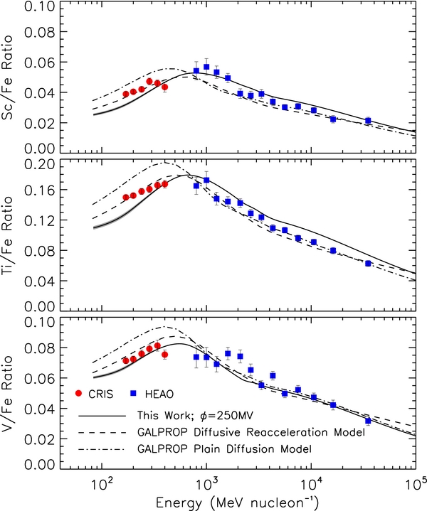
Figure 12. CRIS Sc/Fe, Ti/Fe, and V/Fe ratios for the 2009–2010 solar minimum period (circles). See the caption of Figure 11 for information on the models shown here.
Download figure:
Standard image High-resolution imageIt may be possible to obtain better fits to all of these ratios by adjusting the nuclear fragmentation cross sections used in the transport code. Lave (2012) has shown that the few available measurements for the most important reactions producing 10B and 11B may allow for adjustments up to ∼10%. However, further measurements are required between ∼300 MeV nucleon−1 to a few GeV nucleon−1 in order to better characterize these cross sections. Similar adjustments to the cross sections for producing scandium, titanium, and vanadium may also be possible given the uncertainties in the available measurements (typically ∼10% or larger).
In Figures 11 and 12 our transport model results are also compared with two commonly-used GALPROP numerical models (Version 54.1.984; Strong & Moskalenko 1998; Strong et al. 2009), which have been made available at http://galprop.stanford.edu/webrun/. The first model, shown by the dot-dashed lines, is a plain diffusion model (parameter file galdef_44_999726pub) that is most similar to our leaky-box model since both models do not include interstellar convection and reacceleration. The second model, shown by the dashed line, is a conventional diffusive reacceleration model (parameter file galdef_44_599278pub). The same assumed source abundances used in our model were used in both GALPROP models.
While we have used the Fisk model for our calculations, the GALPROP models presented here used a modulation calculation employing the force-field approximation (hereafter referred to as FF; see Section 6.2) with ϕ = 250 MV. To assess the effects of the different solar modulation models, we have recalculated both the B/C and (Sc+Ti+V)/Fe ratios using our modeled ISM spectra and the FF model. We find that during the 2009–2010 solar minimum the ratios are <4% higher than those obtained using the Fisk model in the CRIS energy range of ∼70–400 MeV nucleon−1.5
Above 1000 MeV nucleon−1 both GALPROP models fit the ratios fairly well, but it is at lower energies that the two models diverge. The plain diffusion model predicts ratios that are much higher than both the CRIS ratios and our leaky-box model results. The differences between the two models are perhaps due to the treatment of cosmic-ray diffusion in the Galaxy. While our model assumes that all particles have an equal probability of escaping the Galaxy no matter their location, the GALPROP models require that particles diffuse to the edge of the Galaxy to escape.
The diffusive reacceleration model is more successful than the plain diffusion model at predicting the ratios at CRIS energies. For the (Sc+Ti+V)/Fe ratio, the reacceleration model gives a very good fit to the data. When looking at the individual parts of this ratio, this model best fits Sc/Fe and Ti/Fe; for V/Fe the data are equally well fit by the reacceleration model and our leaky-box model. We expect that this model would still fit the data well if we had applied the Fisk model for solar modulation instead of the force-field approximation. These results may provide support for the suggestions that some amount of reacceleration in the Galaxy is occurring at low energies.
However, there are still large discrepancies between the reacceleration model and the observed low-energy B/C ratio. That this ratio is better fit using our leaky-box model than the diffusive reacceleration model is unsurprising since the energy dependence of our mean free path for escape from the Galaxy is tailored to provide a good fit to the data. We postulate that the energy dependence we have used here may actually mimic the effect of reacceleration.
7. SUMMARY
We have reported new CRIS measurements of the elemental composition and energy spectra for GCRs from boron to nickel during the 2009–2010 solar minimum period. Measurements for the 1997–1998 solar minimum and the 2001–2003 solar maximum, previously reported in George et al. (2009), are updated here following several improvements to the data analysis. The new 2009–2010 data are shown to be consistent with other experimental data once the differences in the modulation levels are taken into account.
Using a simple leaky-box Galactic transport model combined with a spherically symmetric solar modulation model, we are able to obtain good fits to the secondary-to-primary ratios B/C and (Sc+Ti+V)/Fe and the relevant energy spectra. Though there are some disagreements between the model and the data, the differences may be smaller than the uncertainties attributable to the production cross sections used to account for nuclear fragmentation in the ISM. Our model results are also shown to be comparable to a GALPROP numerical model that includes the effects of diffusive reacceleration in the Galaxy.
This work was supported by NASA at the California Institute of Technology (under grants NNX08AI11G and NNX10AE45G), the Goddard Space Flight Center, the Jet Propulsion Laboratory, and Washington University in Saint Louis. We also acknowledge Dr. Nasser Barghouty for his vital help in updating the semi-empirical nuclear production cross sections used in our interstellar transport code.
APPENDIX A: INTENSITY CALCULATION
At the top of the CRIS instrument, the absolute intensity of GCRs is given by

Here N is the number of counts detected in tlive seconds, AΩ is the geometrical acceptance (in cm2 sr) of the instrument, Δε is the energy interval (MeV nucleon−1),  spall is the correction for nuclear spallation in the instrument, and SOFT is the efficiency of the hodoscope. Intensities for each species are reported in seven energy bins corresponding to particles stopping within detectors E2–E8.
George et al. (2009) describe each of these contributions to the intensity in detail. In Appendix A.1 we discuss new updates to the calculation, including corrections to our Monte Carlo calculation, new parameterizations for the SOFT efficiencies, and changes to the time periods used for the 1997–1998 solar minimum period.
A.1. Updates to the Calculation
The geometrical acceptance of the instrument is calculated using a Monte Carlo simulation that replicates the same cuts used in the data selection. In this update we have corrected small errors in the calculation of the amount of material in the instrument, the exact positioning of the silicon detectors below the hodoscope, and the application of margin cuts to the edge of the hodoscope. The overall effect on the geometrical acceptance and energy bands is small, of the order of ∼1% change to these values.
The corrections we have made to the detector thickness calculation in the Monte Carlo also affect the number of events selected for analysis, since all particles are required to stop more than 160 μm from the top and bottom faces of the detector in order to avoid significant effects of surface dead layers on the energy loss measurements (George et al. 2009). Using the 1997–1998 solar minimum period to test these cuts, we found that for abundant species such as carbon, oxygen, silicon, and iron, the number of selected events changed by less than ∼1%. The number of events for the rarer species, such as phosphorus, chlorine, and scandium, changed by less than ∼3%, while the number of cobalt events (the most statistic-limited species) changed by less than ∼5%. We note that these differences are due to statistical variations; no species-dependent effects were introduced by these cuts.
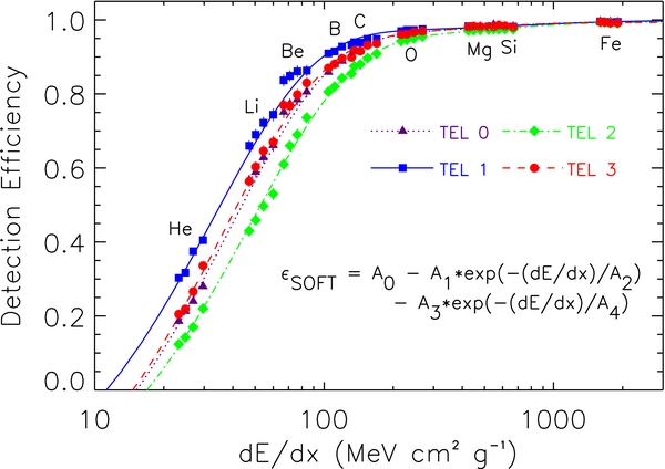
We have also adopted new parameterizations for the SOFT efficiencies based on the work of de Nolfo et al. (2006). Figure 13 shows the efficiencies for each of the four telescopes as a function of the specific ionization at the top of the instrument. Table 3 gives the coefficients for the parameterizations used to fit the data. Though the efficiencies for helium, lithium, and beryllium are shown, they are not used in this work. The efficiencies for the four telescopes are expected to differ, presumably due to photon transmission efficiencies through different lengths of the scintillating optical fibers. Telescope 1 is closest to the camera (Stone et al. 1998a), and therefore has the highest efficiencies; telescope 2 is farthest and has the lowest efficiencies.
Figure 13. The SOFT hodoscope efficiencies by telescope as a function of the specific ionization at the top of the instrument. Selected data include particles stopping in detectors E5–E8. Also shown are fits to the data using the functional form given by the equation, which uses the coefficients A0–A4 given in Table 3.
Download figure:
Standard image High-resolution image
Table 3. SOFT Hodoscope Efficiency Parameterization By Telescope
 | |||||
|---|---|---|---|---|---|
| Telescope | A0 | A1 | A2 | A3 | A4 |
| 0 | 0.996 | 1.407 | 38.68 | 0.049 | 442.3 |
| 1 | 0.998 | 1.359 | 33.00 | 0.034 | 741.5 |
| 2 | 0.995 | 1.335 | 47.91 | 0.059 | 505.2 |
| 3 | 0.993 | 1.410 | 36.37 | 0.054 | 336.5 |
Note. dE/dx, which has been corrected for incident angle, is given in units of MeV cm2 g−1.
Download table as: ASCIITypeset image
With these new formulae the changes to the SOFT efficiencies will be largest for the low-Z species. For boron the efficiencies change by as much as 1.5%, while the efficiencies for heavier species change by less than 0.7%. The heaviest species, such as iron, see the smallest changes to the SOFT efficiencies (less than 0.2%).
Finally, in our previous work we selected data taken from 1997 August 28 to 1998 April 20 for the 1997–1998 solar minimum period. During this time, some high-Z particles were rejected from our analysis because the number of pixels in the event exceeded the pixel threshold set for the image intensifier. On 1997 December 4 this threshold was increased to its current level. The data collected prior to this change should have been excluded from the analysis to avoid a bias in the high-Z data. The new intensities for data collected between 1997 December 5 and 1998 April 20 are reported in Appendix B in Tables 4 and 7.
Table 4. CRIS 1997–1998 Solar Minimum Spectra
| Element | Energies (MeV nucleon−1) | ||||||
|---|---|---|---|---|---|---|---|
| 1997–1998 Intensities (10−9 [cm2 s sr MeV nucleon−1]−1) | |||||||
| B | 59.6 | 79.7 | 102.0 | 121.1 | 138.2 | 154.0 | 168.6 |
| 108.9 ± 4.0 | 132.2 ± 4.4 | 156.2 ± 5.5 | 163.4 ± 6.1 | 183.3 ± 7.3 | 192.5 ± 8.1 | 196.4 ± 8.8 | |
| C | 68.3 | 91.5 | 117.3 | 139.3 | 159.1 | 177.4 | 194.5 |
| 514.9 ± 15.6 | 610.6 ± 18.5 | 710.9 ± 22.5 | 756.0 ± 25.4 | 787.5 ± 27.8 | 802.8 ± 30.3 | 795.5 ± 32.2 | |
| N | 73.3 | 98.1 | 125.9 | 149.6 | 171.0 | 190.7 | 209.2 |
| 125.1 ± 4.3 | 144.1 ± 4.7 | 172.6 ± 6.0 | 180.3 ± 6.6 | 189.7 ± 7.5 | 199.2 ± 8.4 | 186.5 ± 8.5 | |
| O | 80.4 | 107.8 | 138.4 | 164.7 | 188.4 | 210.3 | 230.8 |
| 574.4 ± 17.2 | 665.0 ± 20.2 | 745.7 ± 23.8 | 769.6 ± 26.1 | 779.0 ± 28.7 | 797.2 ± 31.5 | 754.4 ± 32.0 | |
| F | 83.5 | 112.0 | 143.8 | 171.1 | 195.9 | 218.7 | 240.0 |
| 7.6 ± 0.6 | 8.4 ± 0.5 | 10.6 ± 0.7 | 11.5 ± 0.8 | 11.6 ± 0.9 | 11.6 ± 1.0 | 11.6 ± 1.0 | |
| Ne | 89.5 | 120.1 | 154.4 | 183.9 | 210.6 | 235.3 | 258.4 |
| 82.3 ± 2.9 | 95.8 ± 3.2 | 108.0 ± 3.9 | 114.8 ± 4.5 | 113.1 ± 4.8 | 111.3 ± 5.2 | 111.6 ± 5.6 | |
| Na | 94.0 | 126.2 | 162.4 | 193.5 | 221.7 | 247.8 | 272.3 |
| 16.3 ± 0.9 | 19.5 ± 0.9 | 21.0 ± 1.0 | 20.2 ± 1.1 | 21.3 ± 1.3 | 22.6 ± 1.5 | 21.6 ± 1.5 | |
| Mg | 100.2 | 134.7 | 173.4 | 206.8 | 237.1 | 265.2 | 291.5 |
| 119.2 ± 4.0 | 137.3 ± 4.5 | 150.0 ± 5.3 | 161.1 ± 6.2 | 156.1 ± 6.5 | 155.7 ± 7.1 | 146.5 ± 7.3 | |
| Al | 103.8 | 139.6 | 179.8 | 214.5 | 246.1 | 275.3 | 302.8 |
| 16.4 ± 0.9 | 19.9 ± 0.9 | 23.3 ± 1.1 | 21.6 ± 1.2 | 23.3 ± 1.3 | 22.5 ± 1.4 | 21.0 ± 1.5 | |
| Si | 110.1 | 148.2 | 191.1 | 228.1 | 261.8 | 293.1 | 322.6 |
| 90.0 ± 3.1 | 105.1 ± 3.5 | 112.0 ± 4.1 | 113.5 ± 4.5 | 116.2 ± 5.0 | 114.5 ± 5.5 | 103.4 ± 5.4 | |
| P | 112.7 | 151.8 | 195.9 | 233.9 | 268.6 | 300.8 | 331.1 |
| 2.4 ± 0.3 | 2.8 ± 0.2 | 3.3 ± 0.3 | 3.1 ± 0.3 | 3.0 ± 0.4 | 3.0 ± 0.4 | 3.5 ± 0.5 | |
| S | 118.2 | 159.4 | 205.8 | 245.9 | 282.5 | 316.6 | 348.7 |
| 14.1 ± 0.7 | 16.4 ± 0.7 | 18.3 ± 0.9 | 19.5 ± 1.0 | 18.4 ± 1.1 | 18.6 ± 1.2 | 17.3 ± 1.3 | |
| Cl | 120.2 | 162.1 | 209.4 | 250.3 | 287.7 | 322.4 | 355.1 |
| 2.6 ± 0.3 | 2.4 ± 0.2 | 3.0 ± 0.3 | 3.2 ± 0.3 | 3.6 ± 0.4 | 3.3 ± 0.4 | 3.0 ± 0.4 | |
| Ar | 125.0 | 168.8 | 218.1 | 260.9 | 300.0 | 336.4 | 370.8 |
| 5.6 ± 0.4 | 6.5 ± 0.4 | 6.5 ± 0.4 | 7.6 ± 0.5 | 8.2 ± 0.6 | 7.6 ± 0.7 | 7.0 ± 0.7 | |
| K | 127.9 | 172.8 | 223.4 | 267.4 | 307.5 | 344.9 | 380.3 |
| 3.7 ± 0.3 | 4.4 ± 0.3 | 5.3 ± 0.4 | 5.5 ± 0.4 | 5.8 ± 0.5 | 6.2 ± 0.6 | 5.5 ± 0.6 | |
| Ca | 131.6 | 177.9 | 230.1 | 275.6 | 317.1 | 355.9 | 392.4 |
| 11.8 ± 0.6 | 14.7 ± 0.7 | 15.7 ± 0.8 | 16.4 ± 0.9 | 16.2 ± 1.0 | 16.3 ± 1.1 | 15.7 ± 1.2 | |
| Sc | 133.5 | 180.5 | 233.7 | 279.9 | 322.2 | 361.6 | 398.8 |
| 2.9 ± 0.3 | 2.9 ± 0.2 | 3.2 ± 0.3 | 3.6 ± 0.3 | 3.1 ± 0.3 | 3.3 ± 0.4 | 3.3 ± 0.4 | |
| Ti | 137.1 | 185.5 | 240.3 | 287.9 | 331.6 | 372.3 | 410.8 |
| 10.2 ± 0.6 | 11.6 ± 0.6 | 12.7 ± 0.7 | 12.1 ± 0.7 | 12.0 ± 0.8 | 11.4 ± 0.9 | 11.5 ± 0.9 | |
| V | 139.9 | 189.5 | 245.5 | 294.3 | 339.1 | 380.8 | 420.3 |
| 4.5 ± 0.4 | 5.5 ± 0.3 | 5.6 ± 0.4 | 5.8 ± 0.5 | 6.4 ± 0.5 | 5.0 ± 0.5 | 5.6 ± 0.6 | |
| Cr | 144.0 | 195.1 | 253.0 | 303.5 | 349.8 | 393.0 | 434.0 |
| 10.5 ± 0.6 | 11.4 ± 0.5 | 11.1 ± 0.6 | 11.5 ± 0.7 | 11.5 ± 0.8 | 10.6 ± 0.8 | 10.2 ± 0.9 | |
| Mn | 146.8 | 199.1 | 258.3 | 309.9 | 357.3 | 401.6 | 443.5 |
| 6.8 ± 0.4 | 6.8 ± 0.4 | 7.7 ± 0.5 | 7.0 ± 0.5 | 7.2 ± 0.6 | 6.3 ± 0.6 | 5.5 ± 0.6 | |
| Fe | 150.4 | 204.1 | 265.0 | 318.1 | 366.9 | 412.6 | 455.9 |
| 71.6 ± 2.5 | 76.5 ± 2.7 | 76.2 ± 3.0 | 72.8 ± 3.3 | 69.5 ± 3.5 | 64.8 ± 3.8 | 59.2 ± 3.8 | |
| Co | 153.6 | 208.5 | 270.9 | 325.3 | 375.4 | 422.3 | 466.7 |
| 0.62 ± 0.12 | 0.38 ± 0.07 | 0.50 ± 0.10 | 0.47 ± 0.11 | 0.49 ± 0.12 | 0.39 ± 0.12 | 0.47 ± 0.14 | |
| Ni | 158.9 | 215.9 | 280.7 | 337.3 | 389.5 | 438.4 | 484.7 |
| 3.5 ± 0.3 | 3.5 ± 0.2 | 3.7 ± 0.3 | 3.7 ± 0.3 | 3.4 ± 0.3 | 3.0 ± 0.4 | 3.3 ± 0.4 | |
Note. Systematic and statistical uncertainties are combined in quadrature.
Download table as: ASCIITypeset image
Taking into account the above improvements to the analysis, we find that for most species the intensities for both the 1997–1998 solar minimum and 2001–2003 solar maximum have generally changed by less than ∼7%. The relative abundances for these time periods have changed by less than ∼4% for nearly all species.
APPENDIX B: CRIS ENERGY SPECTRA AND COMPOSITION
This appendix provides the CRIS energy spectra for the new 2009–2010 solar minimum. Since Appendix A.1 discusses recent updates to our data analysis that directly affect the results made available in George et al. (2009), we have tabulated the updated energy spectra and composition for those time periods as well.
Table 4 gives the updated spectra for the 1997–1998 solar minimum period, now using data taken from 1997 December 5 to 1998 April 20. Table 5 gives the updated spectra for the 2001–2003 solar maximum period, using data taken from 2001 May 1 to 2003 September 1. The new results presented in this work for the 2009–2010 solar minimum period, using data taken from 2009 March 23 to 2010 January 13, are plotted in Figure 3 and are given in Table 6.
Table 5. CRIS 2001–2003 Solar Maximum Spectra
| Element | Energies (MeV nucleon−1) | ||||||
|---|---|---|---|---|---|---|---|
| 2001–2003 Intensities (10−9 [cm2 s sr MeV nucleon−1]−1) | |||||||
| B | 59.6 | 79.7 | 102.0 | 121.1 | 138.2 | 154.0 | 168.6 |
| 29.8 ± 1.0 | 36.1 ± 1.1 | 43.3 ± 1.4 | 49.6 ± 1.7 | 53.7 ± 2.0 | 58.3 ± 2.3 | 59.2 ± 2.5 | |
| C | 68.3 | 91.5 | 117.3 | 139.3 | 159.1 | 177.4 | 194.5 |
| 109.3 ± 3.3 | 134.5 ± 4.0 | 163.5 ± 5.1 | 183.1 ± 6.1 | 201.0 ± 7.0 | 207.1 ± 7.7 | 215.6 ± 8.6 | |
| N | 73.3 | 98.1 | 125.9 | 149.6 | 171.0 | 190.7 | 209.2 |
| 31.2 ± 1.0 | 37.7 ± 1.2 | 46.7 ± 1.6 | 52.3 ± 1.8 | 56.4 ± 2.1 | 59.8 ± 2.4 | 59.6 ± 2.6 | |
| O | 80.4 | 107.8 | 138.4 | 164.7 | 188.4 | 210.3 | 230.8 |
| 122.2 ± 3.6 | 148.7 ± 4.5 | 180.3 ± 5.7 | 194.5 ± 6.5 | 208.5 ± 7.6 | 217.5 ± 8.5 | 220.5 ± 9.2 | |
| F | 83.5 | 112.0 | 143.8 | 171.1 | 195.9 | 218.7 | 240.0 |
| 2.3 ± 0.1 | 3.0 ± 0.1 | 3.4 ± 0.2 | 3.8 ± 0.2 | 4.0 ± 0.2 | 4.2 ± 0.3 | 4.4 ± 0.3 | |
| Ne | 89.5 | 120.1 | 154.4 | 183.9 | 210.6 | 235.3 | 258.4 |
| 20.6 ± 0.7 | 25.6 ± 0.8 | 30.3 ± 1.0 | 32.8 ± 1.2 | 36.6 ± 1.5 | 37.5 ± 1.6 | 36.5 ± 1.7 | |
| Na | 94.0 | 126.2 | 162.4 | 193.5 | 221.7 | 247.8 | 272.3 |
| 4.5 ± 0.2 | 5.5 ± 0.2 | 6.4 ± 0.3 | 6.6 ± 0.3 | 7.3 ± 0.4 | 7.8 ± 0.4 | 7.9 ± 0.5 | |
| Mg | 100.2 | 134.7 | 173.4 | 206.8 | 237.1 | 265.2 | 291.5 |
| 29.1 ± 0.9 | 35.8 ± 1.1 | 42.3 ± 1.4 | 45.8 ± 1.7 | 48.0 ± 1.9 | 50.9 ± 2.2 | 49.8 ± 2.4 | |
| Al | 103.8 | 139.6 | 179.8 | 214.5 | 246.1 | 275.3 | 302.8 |
| 4.7 ± 0.2 | 6.0 ± 0.2 | 7.1 ± 0.3 | 7.9 ± 0.4 | 8.4 ± 0.4 | 8.0 ± 0.4 | 8.6 ± 0.5 | |
| Si | 110.1 | 148.2 | 191.1 | 228.1 | 261.8 | 293.1 | 322.6 |
| 23.4 ± 0.8 | 28.0 ± 0.9 | 32.4 ± 1.1 | 34.3 ± 1.3 | 36.6 ± 1.5 | 38.7 ± 1.8 | 38.1 ± 1.9 | |
| P | 112.7 | 151.8 | 195.9 | 233.9 | 268.6 | 300.8 | 331.1 |
| 0.7 ± 0.1 | 1.1 ± 0.1 | 1.1 ± 0.1 | 1.3 ± 0.1 | 1.4 ± 0.1 | 1.6 ± 0.1 | 1.7 ± 0.1 | |
| S | 118.2 | 159.4 | 205.8 | 245.9 | 282.5 | 316.6 | 348.7 |
| 4.2 ± 0.2 | 5.1 ± 0.2 | 6.3 ± 0.3 | 7.0 ± 0.3 | 6.9 ± 0.3 | 7.5 ± 0.4 | 7.6 ± 0.4 | |
| Cl | 120.2 | 162.1 | 209.4 | 250.3 | 287.7 | 322.4 | 355.1 |
| 0.9 ± 0.1 | 1.1 ± 0.1 | 1.4 ± 0.1 | 1.4 ± 0.1 | 1.6 ± 0.1 | 1.9 ± 0.1 | 1.8 ± 0.1 | |
| Ar | 125.0 | 168.8 | 218.1 | 260.9 | 300.0 | 336.4 | 370.8 |
| 1.9 ± 0.1 | 2.3 ± 0.1 | 2.8 ± 0.1 | 3.2 ± 0.2 | 3.3 ± 0.2 | 3.4 ± 0.2 | 3.1 ± 0.2 | |
| K | 127.9 | 172.8 | 223.4 | 267.4 | 307.5 | 344.9 | 380.3 |
| 1.6 ± 0.1 | 1.8 ± 0.1 | 2.2 ± 0.1 | 2.5 ± 0.1 | 2.5 ± 0.2 | 2.6 ± 0.2 | 2.7 ± 0.2 | |
| Ca | 131.6 | 177.9 | 230.1 | 275.6 | 317.1 | 355.9 | 392.4 |
| 4.0 ± 0.2 | 5.0 ± 0.2 | 5.6 ± 0.2 | 6.0 ± 0.3 | 6.5 ± 0.3 | 6.6 ± 0.4 | 6.7 ± 0.4 | |
| Sc | 133.5 | 180.5 | 233.7 | 279.9 | 322.2 | 361.6 | 398.8 |
| 0.9 ± 0.1 | 1.1 ± 0.1 | 1.3 ± 0.1 | 1.3 ± 0.1 | 1.4 ± 0.1 | 1.4 ± 0.1 | 1.4 ± 0.1 | |
| Ti | 137.1 | 185.5 | 240.3 | 287.9 | 331.6 | 372.3 | 410.8 |
| 3.3 ± 0.1 | 4.0 ± 0.2 | 4.4 ± 0.2 | 4.6 ± 0.2 | 4.6 ± 0.3 | 4.9 ± 0.3 | 4.6 ± 0.3 | |
| V | 139.9 | 189.5 | 245.5 | 294.3 | 339.1 | 380.8 | 420.3 |
| 1.5 ± 0.1 | 1.8 ± 0.1 | 2.0 ± 0.1 | 2.1 ± 0.1 | 2.2 ± 0.1 | 2.1 ± 0.2 | 2.3 ± 0.2 | |
| Cr | 144.0 | 195.1 | 253.0 | 303.5 | 349.8 | 393.0 | 434.0 |
| 3.0 ± 0.1 | 3.7 ± 0.2 | 4.0 ± 0.2 | 4.1 ± 0.2 | 4.4 ± 0.3 | 4.4 ± 0.3 | 4.1 ± 0.3 | |
| Mn | 146.8 | 199.1 | 258.3 | 309.9 | 357.3 | 401.6 | 443.5 |
| 2.0 ± 0.1 | 2.1 ± 0.1 | 2.7 ± 0.1 | 2.7 ± 0.2 | 2.8 ± 0.2 | 2.9 ± 0.2 | 2.6 ± 0.2 | |
| Fe | 150.4 | 204.1 | 265.0 | 318.1 | 366.9 | 412.6 | 455.9 |
| 21.2 ± 0.7 | 23.9 ± 0.8 | 26.7 ± 1.0 | 27.6 ± 1.2 | 28.9 ± 1.4 | 28.6 ± 1.6 | 28.2 ± 1.7 | |
| Co | 153.6 | 208.5 | 270.9 | 325.3 | 375.4 | 422.3 | 466.7 |
| 0.09 ± 0.02 | 0.15 ± 0.02 | 0.19 ± 0.02 | 0.17 ± 0.03 | 0.18 ± 0.03 | 0.20 ± 0.04 | 0.20 ± 0.04 | |
| Ni | 158.9 | 215.9 | 280.7 | 337.3 | 389.5 | 438.4 | 484.7 |
| 1.0 ± 0.1 | 1.2 ± 0.1 | 1.3 ± 0.1 | 1.3 ± 0.1 | 1.6 ± 0.1 | 1.5 ± 0.1 | 1.4 ± 0.1 | |
Note. Systematic and statistical uncertainties are combined in quadrature.
Download table as: ASCIITypeset image
Table 6. CRIS 2009–2010 Solar Minimum Spectra
| Element | Energies (MeV nucleon−1) | ||||||
|---|---|---|---|---|---|---|---|
| 2009–2010 Intensities (10−9 [cm2 s sr MeV nucleon−1]−1) | |||||||
| B | 59.6 | 79.7 | 102.0 | 121.1 | 138.2 | 154.0 | 168.6 |
| 132.2 ± 4.3 | 155.9 ± 4.9 | 186.8 ± 6.1 | 199.7 ± 6.9 | 213.4 ± 7.9 | 233.0 ± 9.1 | 226.8 ± 9.5 | |
| C | 68.3 | 91.5 | 117.3 | 139.3 | 159.1 | 177.4 | 194.5 |
| 638.0 ± 18.8 | 762.9 ± 22.7 | 888.1 ± 27.7 | 924.9 ± 30.5 | 976.4 ± 33.8 | 969.1 ± 35.9 | 961.5 ± 38.2 | |
| N | 73.3 | 98.1 | 125.9 | 149.6 | 171.0 | 190.7 | 209.2 |
| 150.4 ± 4.7 | 176.9 ± 5.4 | 204.6 ± 6.6 | 219.8 ± 7.6 | 231.0 ± 8.5 | 232.5 ± 9.2 | 228.2 ± 9.7 | |
| O | 80.4 | 107.8 | 138.4 | 164.7 | 188.4 | 210.3 | 230.8 |
| 704.5 ± 20.5 | 831.4 ± 24.9 | 920.5 ± 28.9 | 946.6 ± 31.5 | 966.2 ± 34.9 | 959.2 ± 37.2 | 924.0 ± 38.5 | |
| F | 83.5 | 112.0 | 143.8 | 171.1 | 195.9 | 218.7 | 240.0 |
| 9.7 ± 0.5 | 11.6 ± 0.5 | 12.2 ± 0.6 | 13.3 ± 0.7 | 13.2 ± 0.7 | 14.6 ± 0.9 | 14.8 ± 0.9 | |
| Ne | 89.5 | 120.1 | 154.4 | 183.9 | 210.6 | 235.3 | 258.4 |
| 101.4 ± 3.2 | 115.9 ± 3.6 | 134.2 ± 4.5 | 135.3 ± 4.9 | 137.7 ± 5.4 | 140.4 ± 6.0 | 131.8 ± 6.1 | |
| Na | 94.0 | 126.2 | 162.4 | 193.5 | 221.7 | 247.8 | 272.3 |
| 19.3 ± 0.8 | 21.9 ± 0.8 | 24.8 ± 1.0 | 26.6 ± 1.1 | 26.4 ± 1.2 | 25.9 ± 1.3 | 27.3 ± 1.5 | |
| Mg | 100.2 | 134.7 | 173.4 | 206.8 | 237.1 | 265.2 | 291.5 |
| 149.3 ± 4.6 | 171.8 ± 5.3 | 185.2 ± 6.2 | 189.0 ± 6.9 | 187.6 ± 7.5 | 185.2 ± 8.0 | 178.2 ± 8.4 | |
| Al | 103.8 | 139.6 | 179.8 | 214.5 | 246.1 | 275.3 | 302.8 |
| 22.1 ± 0.8 | 25.3 ± 0.9 | 28.3 ± 1.1 | 28.2 ± 1.2 | 28.1 ± 1.3 | 30.0 ± 1.5 | 27.4 ± 1.5 | |
| Si | 110.1 | 148.2 | 191.1 | 228.1 | 261.8 | 293.1 | 322.6 |
| 112.3 ± 3.5 | 128.1 ± 4.0 | 137.2 ± 4.7 | 139.3 ± 5.2 | 135.5 ± 5.5 | 132.9 ± 6.0 | 125.1 ± 6.2 | |
| P | 112.7 | 151.8 | 195.9 | 233.9 | 268.6 | 300.8 | 331.1 |
| 2.9 ± 0.2 | 3.3 ± 0.2 | 4.1 ± 0.2 | 3.9 ± 0.3 | 4.4 ± 0.3 | 4.1 ± 0.3 | 4.3 ± 0.4 | |
| S | 118.2 | 159.4 | 205.8 | 245.9 | 282.5 | 316.6 | 348.7 |
| 17.9 ± 0.7 | 20.3 ± 0.7 | 22.2 ± 0.9 | 23.7 ± 1.0 | 22.6 ± 1.1 | 22.0 ± 1.2 | 21.1 ± 1.2 | |
| Cl | 120.2 | 162.1 | 209.4 | 250.3 | 287.7 | 322.4 | 355.1 |
| 2.8 ± 0.2 | 3.0 ± 0.2 | 4.1 ± 0.2 | 3.9 ± 0.3 | 4.2 ± 0.3 | 4.0 ± 0.3 | 3.8 ± 0.3 | |
| Ar | 125.0 | 168.8 | 218.1 | 260.9 | 300.0 | 336.4 | 370.8 |
| 6.0 ± 0.3 | 7.6 ± 0.3 | 8.7 ± 0.4 | 9.0 ± 0.5 | 9.6 ± 0.6 | 8.8 ± 0.6 | 9.7 ± 0.7 | |
| K | 127.9 | 172.8 | 223.4 | 267.4 | 307.5 | 344.9 | 380.3 |
| 4.8 ± 0.3 | 5.4 ± 0.3 | 6.1 ± 0.3 | 6.6 ± 0.4 | 7.0 ± 0.4 | 7.0 ± 0.5 | 6.9 ± 0.5 | |
| Ca | 131.6 | 177.9 | 230.1 | 275.6 | 317.1 | 355.9 | 392.4 |
| 14.4 ± 0.6 | 16.3 ± 0.6 | 18.7 ± 0.8 | 17.7 ± 0.8 | 19.4 ± 1.0 | 19.6 ± 1.1 | 18.8 ± 1.2 | |
| Sc | 133.5 | 180.5 | 233.7 | 279.9 | 322.2 | 361.6 | 398.8 |
| 2.9 ± 0.2 | 3.6 ± 0.2 | 3.8 ± 0.2 | 4.3 ± 0.3 | 3.9 ± 0.3 | 4.0 ± 0.3 | 3.5 ± 0.3 | |
| Ti | 137.1 | 185.5 | 240.3 | 287.9 | 331.6 | 372.3 | 410.8 |
| 12.6 ± 0.5 | 13.8 ± 0.5 | 14.6 ± 0.6 | 14.5 ± 0.7 | 14.3 ± 0.8 | 13.9 ± 0.8 | 13.0 ± 0.9 | |
| V | 139.9 | 189.5 | 245.5 | 294.3 | 339.1 | 380.8 | 420.3 |
| 6.1 ± 0.3 | 6.6 ± 0.3 | 7.1 ± 0.4 | 7.2 ± 0.4 | 7.0 ± 0.4 | 5.5 ± 0.4 | 6.4 ± 0.5 | |
| Cr | 144.0 | 195.1 | 253.0 | 303.5 | 349.8 | 393.0 | 434.0 |
| 12.5 ± 0.5 | 13.8 ± 0.5 | 13.8 ± 0.6 | 13.9 ± 0.7 | 12.4 ± 0.7 | 11.6 ± 0.7 | 12.1 ± 0.8 | |
| Mn | 146.8 | 199.1 | 258.3 | 309.9 | 357.3 | 401.6 | 443.5 |
| 8.0 ± 0.4 | 8.5 ± 0.4 | 8.7 ± 0.4 | 8.3 ± 0.4 | 7.7 ± 0.5 | 8.1 ± 0.6 | 7.2 ± 0.6 | |
| Fe | 150.4 | 204.1 | 265.0 | 318.1 | 366.9 | 412.6 | 455.9 |
| 87.7 ± 2.8 | 92.3 ± 3.0 | 92.4 ± 3.5 | 87.3 ± 3.7 | 83.8 ± 4.0 | 77.5 ± 4.3 | 70.1 ± 4.3 | |
| Co | 153.6 | 208.5 | 270.9 | 325.3 | 375.4 | 422.3 | 466.7 |
| 0.48 ± 0.07 | 0.53 ± 0.06 | 0.54 ± 0.07 | 0.54 ± 0.08 | 0.59 ± 0.09 | 0.49 ± 0.09 | 0.51 ± 0.10 | |
| Ni | 158.9 | 215.9 | 280.7 | 337.3 | 389.5 | 438.4 | 484.7 |
| 4.0 ± 0.2 | 4.5 ± 0.2 | 4.3 ± 0.2 | 4.6 ± 0.3 | 4.1 ± 0.3 | 3.6 ± 0.3 | 3.4 ± 0.3 | |
Note. Systematic and statistical uncertainties are combined in quadrature.
Download table as: ASCIITypeset image
For convenience, these data have also been linearly interpolated between adjacent data points in log(Intensity) versus log(Energy/nucleon) to a common energy grid. The interpolated spectra for the 1997–1998 solar minimum, 2001–2003 solar maximum, and 2009–2010 solar minimum are given in Tables 7, 8, and 9, respectively. In each table, some slightly extrapolated points are included at the high and/or low energies (up to ±5% in energy). The uncertainties on these data are calculated by combining in quadrature the systematic and statistical uncertainties. The statistical contribution is a simple propagation of errors using the statistical uncertainties for the measured points on either side of the interpolated point.
Table 7. CRIS 1997–1998 Solar Minimum Spectra Interpolated to a Common Energy Grid
| Energies (MeV nucleon−1) | |||||||
|---|---|---|---|---|---|---|---|
| 1997–1998 Intensities (10−9 [cm2 s sr MeV nucleon−1]−1) | |||||||
| Element | 60 | 72 | 85 | 100 | 120 | 142 | 170 |
| B | 109.4 ± 4.0 | 123.6 ± 4.0 | 138.1 ± 4.4 | 154.1 ± 5.3 | 163.0 ± 6.0 | 185.5 ± 7.0 | 196.8 ± 9.1 |
| C | 531.0 ± 15.8 | 584.9 ± 17.5 | 644.7 ± 19.3 | 716.7 ± 22.5 | 760.4 ± 25.3 | 796.8 ± 29.6 | |
| N | 124.0 ± 4.4 | 134.4 ± 4.3 | 146.1 ± 4.7 | 166.7 ± 5.6 | 177.9 ± 6.3 | 189.3 ± 7.4 | |
| O | 590.6 ± 17.5 | 640.5 ± 19.3 | 698.5 ± 21.0 | 749.2 ± 23.7 | 771.8 ± 25.9 | ||
| F | 7.7 ± 0.6 | 8.1 ± 0.4 | 8.9 ± 0.5 | 10.5 ± 0.7 | 11.4 ± 0.8 | ||
| Ne | 87.1 ± 2.8 | 95.7 ± 3.2 | 103.7 ± 3.6 | 111.7 ± 4.1 | |||
| Na | 17.0 ± 0.8 | 18.9 ± 0.8 | 20.2 ± 0.8 | 20.8 ± 0.9 | |||
| Mg | 119.1 ± 4.0 | 129.9 ± 4.1 | 139.9 ± 4.4 | 149.0 ± 5.2 | |||
| Al | 16.0 ± 0.9 | 18.0 ± 0.7 | 20.1 ± 0.9 | 22.5 ± 1.0 | |||
| Si | 94.2 ± 3.0 | 102.8 ± 3.3 | 108.8 ± 3.8 | ||||
| P | 2.5 ± 0.2 | 2.7 ± 0.2 | 3.0 ± 0.2 | ||||
| S | 14.2 ± 0.7 | 15.5 ± 0.6 | 16.9 ± 0.7 | ||||
| Cl | 2.6 ± 0.3 | 2.5 ± 0.2 | 2.5 ± 0.2 | ||||
| Ar | 5.5 ± 0.5 | 6.0 ± 0.3 | 6.5 ± 0.4 | ||||
| K | 3.9 ± 0.3 | 4.4 ± 0.3 | |||||
| Ca | 12.5 ± 0.6 | 14.3 ± 0.6 | |||||
| Sc | 2.9 ± 0.2 | 2.9 ± 0.2 | |||||
| Ti | 10.4 ± 0.5 | 11.2 ± 0.5 | |||||
| V | 4.6 ± 0.3 | 5.1 ± 0.3 | |||||
| Cr | 10.5 ± 0.6 | 11.0 ± 0.5 | |||||
| Mn | 6.8 ± 0.5 | 6.8 ± 0.3 | |||||
| Fe | 73.5 ± 2.5 | ||||||
| Co | 0.5 ± 0.1 | ||||||
| Ni | 3.5 ± 0.2 | ||||||
| Energies (MeV nucleon−1) | |||||||
| 1997–1998 Intensities (10−9 [cm2 s sr MeV nucleon−1]−1) | |||||||
| Element | 200 | 240 | 285 | 340 | 400 | 475 | |
| C | 793.4 ± 32.9 | ||||||
| N | 192.6 ± 8.3 | ||||||
| O | 788.8 ± 30.7 | 737.2 ± 32.2 | |||||
| F | 11.6 ± 0.8 | 11.6 ± 1.0 | |||||
| Ne | 113.7 ± 4.5 | 111.4 ± 5.0 | |||||
| Na | 20.5 ± 1.0 | 22.2 ± 1.2 | 21.2 ± 2.0 | ||||
| Mg | 158.9 ± 5.9 | 156.1 ± 6.4 | 148.7 ± 7.2 | ||||
| Al | 22.3 ± 1.0 | 23.0 ± 1.2 | 21.9 ± 1.2 | ||||
| Si | 112.4 ± 3.9 | 114.5 ± 4.3 | 114.9 ± 5.3 | ||||
| P | 3.3 ± 0.3 | 3.1 ± 0.3 | 3.0 ± 0.3 | 3.7 ± 0.6 | |||
| S | 18.1 ± 0.8 | 19.4 ± 1.0 | 18.4 ± 1.1 | 17.6 ± 1.1 | |||
| Cl | 2.9 ± 0.2 | 3.2 ± 0.3 | 3.5 ± 0.4 | 3.2 ± 0.3 | |||
| Ar | 6.5 ± 0.4 | 7.1 ± 0.4 | 8.0 ± 0.5 | 7.6 ± 0.6 | |||
| K | 4.9 ± 0.3 | 5.4 ± 0.3 | 5.6 ± 0.4 | 6.2 ± 0.5 | |||
| Ca | 15.2 ± 0.6 | 15.8 ± 0.7 | 16.3 ± 0.8 | 16.2 ± 1.0 | 15.6 ± 1.3 | ||
| Sc | 3.0 ± 0.2 | 3.3 ± 0.3 | 3.5 ± 0.3 | 3.2 ± 0.3 | 3.3 ± 0.4 | ||
| Ti | 11.9 ± 0.5 | 12.7 ± 0.7 | 12.1 ± 0.7 | 11.9 ± 0.7 | 11.4 ± 0.8 | ||
| V | 5.5 ± 0.3 | 5.6 ± 0.4 | 5.8 ± 0.4 | 6.3 ± 0.5 | 5.3 ± 0.4 | ||
| Cr | 11.3 ± 0.5 | 11.2 ± 0.6 | 11.4 ± 0.6 | 11.5 ± 0.7 | 10.5 ± 0.8 | ||
| Mn | 6.9 ± 0.4 | 7.5 ± 0.4 | 7.3 ± 0.4 | 7.1 ± 0.5 | 6.4 ± 0.6 | ||
| Fe | 76.1 ± 2.6 | 76.3 ± 2.9 | 74.8 ± 2.9 | 71.2 ± 3.5 | 66.0 ± 3.7 | 57.1 ± 4.0 | |
| Co | 0.4 ± 0.1 | 0.4 ± 0.1 | 0.5 ± 0.1 | 0.5 ± 0.1 | 0.4 ± 0.1 | 0.5 ± 0.2 | |
| Ni | 3.5 ± 0.2 | 3.6 ± 0.2 | 3.7 ± 0.3 | 3.7 ± 0.3 | 3.3 ± 0.3 | 3.3 ± 0.3 | |
Note. Systematic and statistical uncertainties are combined in quadrature.
Download table as: ASCIITypeset image
Table 8. CRIS 2001–2003 Solar Maximum Spectra Interpolated to a Common Energy Grid
| Energies (MeV nucleon−1) | |||||||
|---|---|---|---|---|---|---|---|
| 2001–2003 Intensities (10−9 [cm2 s sr MeV nucleon−1]−1) | |||||||
| Element | 60 | 72 | 85 | 100 | 120 | 142 | 170 |
| B | 30.0 ± 1.0 | 33.8 ± 1.0 | 37.9 ± 1.2 | 42.7 ± 1.4 | 49.2 ± 1.7 | 54.8 ± 2.0 | 59.3 ± 2.5 |
| C | 113.5 ± 3.4 | 127.7 ± 3.8 | 144.2 ± 4.3 | 166.0 ± 5.2 | 185.6 ± 6.1 | 204.7 ± 7.5 | |
| N | 30.9 ± 1.0 | 34.3 ± 1.1 | 38.3 ± 1.2 | 44.8 ± 1.5 | 50.6 ± 1.7 | 56.2 ± 2.1 | |
| O | 126.8 ± 3.7 | 141.4 ± 4.2 | 161.5 ± 4.8 | 182.3 ± 5.7 | 197.7 ± 6.6 | ||
| F | 2.4 ± 0.1 | 2.7 ± 0.1 | 3.1 ± 0.1 | 3.4 ± 0.2 | 3.8 ± 0.2 | ||
| Ne | 22.4 ± 0.7 | 25.6 ± 0.8 | 28.6 ± 1.0 | 31.6 ± 1.1 | |||
| Na | 4.7 ± 0.2 | 5.3 ± 0.2 | 5.9 ± 0.2 | 6.5 ± 0.3 | |||
| Mg | 29.0 ± 0.9 | 33.0 ± 1.0 | 37.1 ± 1.2 | 41.8 ± 1.4 | |||
| Al | 4.6 ± 0.2 | 5.3 ± 0.2 | 6.0 ± 0.2 | 6.8 ± 0.3 | |||
| Si | 24.7 ± 0.8 | 27.3 ± 0.9 | 30.3 ± 1.0 | ||||
| P | 0.8 ± 0.1 | 1.0 ± 0.1 | 1.1 ± 0.1 | ||||
| S | 4.3 ± 0.2 | 4.8 ± 0.2 | 5.4 ± 0.2 | ||||
| Cl | 0.9 ± 0.1 | 1.0 ± 0.1 | 1.2 ± 0.1 | ||||
| Ar | 1.9 ± 0.1 | 2.0 ± 0.1 | 2.3 ± 0.1 | ||||
| K | 1.7 ± 0.1 | 1.8 ± 0.1 | |||||
| Ca | 4.2 ± 0.2 | 4.8 ± 0.2 | |||||
| Sc | 0.9 ± 0.1 | 1.1 ± 0.1 | |||||
| Ti | 3.4 ± 0.1 | 3.8 ± 0.1 | |||||
| V | 1.5 ± 0.1 | 1.7 ± 0.1 | |||||
| Cr | 3.0 ± 0.1 | 3.4 ± 0.1 | |||||
| Mn | 2.0 ± 0.1 | 2.1 ± 0.1 | |||||
| Fe | 22.2 ± 0.7 | ||||||
| Co | 0.1 ± 0.0 | ||||||
| Ni | 1.0 ± 0.1 | ||||||
| Energies (MeV nucleon−1) | |||||||
| 2001–2003 Intensities (10−9 [cm2 s sr MeV nucleon−1]−1) | |||||||
| Element | 200 | 240 | 285 | 340 | 400 | 475 | |
| C | 218.3 ± 8.9 | ||||||
| N | 59.7 ± 2.5 | ||||||
| O | 213.3 ± 8.3 | 221.8 ± 9.4 | |||||
| F | 4.0 ± 0.2 | 4.4 ± 0.3 | |||||
| Ne | 35.1 ± 1.4 | 37.3 ± 1.6 | |||||
| Na | 6.8 ± 0.3 | 7.6 ± 0.4 | 7.9 ± 0.6 | ||||
| Mg | 45.1 ± 1.6 | 48.3 ± 1.9 | 50.1 ± 2.4 | ||||
| Al | 7.6 ± 0.3 | 8.3 ± 0.4 | 8.2 ± 0.4 | ||||
| Si | 32.9 ± 1.1 | 35.1 ± 1.3 | 38.2 ± 1.7 | ||||
| P | 1.1 ± 0.1 | 1.3 ± 0.1 | 1.5 ± 0.1 | 1.7 ± 0.2 | |||
| S | 6.1 ± 0.2 | 6.9 ± 0.3 | 6.9 ± 0.3 | 7.6 ± 0.4 | |||
| Cl | 1.4 ± 0.1 | 1.4 ± 0.1 | 1.5 ± 0.1 | 1.8 ± 0.1 | |||
| Ar | 2.6 ± 0.1 | 3.0 ± 0.1 | 3.3 ± 0.2 | 3.3 ± 0.2 | |||
| K | 2.0 ± 0.1 | 2.3 ± 0.1 | 2.5 ± 0.1 | 2.6 ± 0.2 | |||
| Ca | 5.3 ± 0.2 | 5.6 ± 0.2 | 6.1 ± 0.3 | 6.6 ± 0.3 | 6.8 ± 0.5 | ||
| Sc | 1.2 ± 0.1 | 1.3 ± 0.1 | 1.3 ± 0.1 | 1.4 ± 0.1 | 1.4 ± 0.1 | ||
| Ti | 4.1 ± 0.2 | 4.4 ± 0.2 | 4.6 ± 0.2 | 4.7 ± 0.2 | 4.7 ± 0.3 | ||
| V | 1.8 ± 0.1 | 2.0 ± 0.1 | 2.1 ± 0.1 | 2.2 ± 0.1 | 2.2 ± 0.1 | ||
| Cr | 3.7 ± 0.1 | 3.9 ± 0.2 | 4.1 ± 0.2 | 4.4 ± 0.2 | 4.4 ± 0.3 | ||
| Mn | 2.2 ± 0.1 | 2.5 ± 0.1 | 2.7 ± 0.1 | 2.8 ± 0.2 | 2.9 ± 0.2 | ||
| Fe | 23.8 ± 0.8 | 25.6 ± 1.0 | 27.0 ± 1.0 | 28.2 ± 1.3 | 28.7 ± 1.6 | 28.0 ± 1.8 | |
| Co | 0.1 ± 0.0 | 0.2 ± 0.0 | 0.2 ± 0.0 | 0.2 ± 0.0 | 0.2 ± 0.0 | 0.2 ± 0.0 | |
| Ni | 1.2 ± 0.1 | 1.3 ± 0.1 | 1.3 ± 0.1 | 1.4 ± 0.1 | 1.6 ± 0.1 | 1.4 ± 0.1 | |
Note. Systematic and statistical uncertainties are combined in quadrature.
Download table as: ASCIITypeset image
Table 9. CRIS 2009–2010 Solar Minimum Spectra Interpolated to a Common Energy Grid
| Energies (MeV nucleon−1) | |||||||
|---|---|---|---|---|---|---|---|
| 2009–2010 Intensities (10−9 [cm2 s sr MeV nucleon−1]−1) | |||||||
| Element | 60 | 72 | 85 | 100 | 120 | 142 | 170 |
| B | 132.7 ± 4.3 | 147.2 ± 4.5 | 163.4 ± 5.0 | 184.1 ± 6.0 | 199.0 ± 6.9 | 218.2 ± 7.8 | 226.2 ± 9.6 |
| C | 658.9 ± 19.3 | 729.3 ± 21.6 | 805.5 ± 23.9 | 892.9 ± 27.7 | 932.2 ± 30.6 | 971.9 ± 35.7 | |
| N | 148.9 ± 4.6 | 163.3 ± 4.9 | 178.9 ± 5.4 | 199.0 ± 6.4 | 215.1 ± 7.3 | 230.5 ± 8.5 | |
| O | 727.0 ± 21.1 | 796.9 ± 23.8 | 868.5 ± 25.9 | 924.3 ± 29.0 | 951.2 ± 31.6 | ||
| F | 9.8 ± 0.5 | 10.8 ± 0.4 | 11.7 ± 0.5 | 12.2 ± 0.6 | 13.2 ± 0.7 | ||
| Ne | 106.7 ± 3.2 | 115.9 ± 3.6 | 127.8 ± 4.2 | 134.8 ± 4.7 | |||
| Na | 19.8 ± 0.7 | 21.4 ± 0.8 | 23.2 ± 0.8 | 25.3 ± 0.9 | |||
| Mg | 149.2 ± 4.6 | 162.6 ± 5.0 | 174.5 ± 5.3 | 184.2 ± 6.1 | |||
| Al | 21.7 ± 0.9 | 23.6 ± 0.8 | 25.5 ± 0.9 | 27.6 ± 1.0 | |||
| Si | 116.7 ± 3.5 | 125.7 ± 3.9 | 132.9 ± 4.5 | ||||
| P | 3.0 ± 0.2 | 3.2 ± 0.2 | 3.6 ± 0.2 | ||||
| S | 18.0 ± 0.7 | 19.3 ± 0.7 | 20.8 ± 0.7 | ||||
| Cl | 2.8 ± 0.2 | 2.9 ± 0.1 | 3.2 ± 0.2 | ||||
| Ar | 5.8 ± 0.3 | 6.6 ± 0.3 | 7.7 ± 0.3 | ||||
| K | 5.0 ± 0.2 | 5.4 ± 0.2 | |||||
| Ca | 14.9 ± 0.5 | 16.0 ± 0.6 | |||||
| Sc | 3.0 ± 0.2 | 3.5 ± 0.2 | |||||
| Ti | 12.7 ± 0.5 | 13.4 ± 0.5 | |||||
| V | 6.1 ± 0.3 | 6.4 ± 0.3 | |||||
| Cr | 12.5 ± 0.5 | 13.2 ± 0.5 | |||||
| Mn | 7.9 ± 0.4 | 8.2 ± 0.3 | |||||
| Fe | 89.5 ± 2.9 | ||||||
| Co | 0.5 ± 0.1 | ||||||
| Ni | 4.1 ± 0.2 | ||||||
| Energies (MeV nucleon−1) | |||||||
| 2009–2010 Intensities (10−9 [cm2 s sr MeV nucleon−1]−1) | |||||||
| Element | 200 | 240 | 285 | 340 | 400 | 475 | |
| C | 959.2 ± 38.6 | ||||||
| N | 230.3 ± 9.5 | ||||||
| O | 962.4 ± 37.1 | 909.6 ± 38.3 | |||||
| F | 13.5 ± 0.7 | 14.8 ± 0.9 | |||||
| Ne | 136.8 ± 5.2 | 138.6 ± 5.8 | |||||
| Na | 26.6 ± 1.1 | 26.1 ± 1.2 | 28.0 ± 1.9 | ||||
| Mg | 188.3 ± 6.8 | 187.4 ± 7.4 | 179.8 ± 8.4 | ||||
| Al | 28.3 ± 1.1 | 28.1 ± 1.3 | 29.0 ± 1.4 | ||||
| Si | 137.7 ± 4.6 | 137.8 ± 5.0 | 133.5 ± 5.9 | ||||
| P | 4.0 ± 0.2 | 4.0 ± 0.2 | 4.3 ± 0.3 | 4.3 ± 0.5 | |||
| S | 22.0 ± 0.9 | 23.5 ± 1.0 | 22.6 ± 1.1 | 21.3 ± 1.2 | |||
| Cl | 3.9 ± 0.2 | 4.0 ± 0.2 | 4.2 ± 0.3 | 3.9 ± 0.3 | |||
| Ar | 8.3 ± 0.3 | 8.8 ± 0.4 | 9.3 ± 0.5 | 8.9 ± 0.6 | |||
| K | 5.8 ± 0.3 | 6.3 ± 0.3 | 6.8 ± 0.3 | 7.0 ± 0.5 | |||
| Ca | 17.4 ± 0.6 | 18.5 ± 0.7 | 18.1 ± 0.8 | 19.5 ± 1.0 | 18.7 ± 1.2 | ||
| Sc | 3.7 ± 0.2 | 3.9 ± 0.2 | 4.3 ± 0.3 | 3.9 ± 0.3 | 3.4 ± 0.3 | ||
| Ti | 14.0 ± 0.5 | 14.6 ± 0.6 | 14.5 ± 0.7 | 14.2 ± 0.7 | 13.2 ± 0.8 | ||
| V | 6.7 ± 0.3 | 7.0 ± 0.3 | 7.2 ± 0.4 | 7.0 ± 0.4 | 6.0 ± 0.4 | ||
| Cr | 13.8 ± 0.5 | 13.8 ± 0.6 | 13.9 ± 0.6 | 12.7 ± 0.7 | 11.7 ± 0.7 | ||
| Mn | 8.5 ± 0.4 | 8.6 ± 0.4 | 8.5 ± 0.4 | 7.9 ± 0.4 | 8.0 ± 0.5 | ||
| Fe | 92.0 ± 3.0 | 92.4 ± 3.4 | 90.4 ± 3.4 | 85.7 ± 4.1 | 79.1 ± 4.3 | 67.3 ± 4.3 | |
| Co | 0.5 ± 0.1 | 0.5 ± 0.0 | 0.5 ± 0.1 | 0.6 ± 0.1 | 0.5 ± 0.1 | 0.5 ± 0.1 | |
| Ni | 4.4 ± 0.2 | 4.4 ± 0.2 | 4.3 ± 0.2 | 4.6 ± 0.3 | 4.0 ± 0.3 | 3.4 ± 0.3 | |
Note. Systematic and statistical uncertainties are combined in quadrature.
Download table as: ASCIITypeset image
Footnotes
- 5
While these differences are small for the ratios, there are larger disagreements between the Fisk model and the FF model energy spectra at 1 AU. Using our ISM spectra, we find that the solar minimum intensities at 50 MeV nucleon−1 are 6%–12% higher using the FF model than with the Fisk model; these differences decrease with increasing energy. During solar maximum periods, the intensities and the secondary-to-primary ratios are, respectively, 12%–27% and <10% higher using the FF model than with the Fisk model. Caballero-Lopez & Moraal (2004) further discuss the limitations of using the FF model for solar modulation.