


ABSTRACT
It is believed that magnetic helicity conservation is an important constraint on large-scale astrophysical dynamos. In this paper, we study a mean-field solar dynamo model that employs two different formulations of the magnetic helicity conservation. In the first approach, the evolution of the averaged small-scale magnetic helicity is largely determined by the local induction effects due to the large-scale magnetic field, turbulent motions, and the turbulent diffusive loss of helicity. In this case, the dynamo model shows that the typical strength of the large-scale magnetic field generated by the dynamo is much smaller than the equipartition value for the magnetic Reynolds number 106. This is the so-called catastrophic quenching (CQ) phenomenon. In the literature, this is considered to be typical for various kinds of solar dynamo models, including the distributed-type and the Babcock–Leighton-type dynamos. The problem can be resolved by the second formulation, which is derived from the integral conservation of the total magnetic helicity. In this case, the dynamo model shows that magnetic helicity propagates with the dynamo wave from the bottom of the convection zone to the surface. This prevents CQ because of the local balance between the large-scale and small-scale magnetic helicities. Thus, the solar dynamo can operate in a wide range of magnetic Reynolds numbers up to 106.
Export citation and abstract BibTeX RIS
1. INTRODUCTION
The basic idea of the solar dynamo action was developed by Parker (1955). He suggested that the toroidal component of the solar magnetic field is stretched from the poloidal component by the differential rotation (Ω-effect), and the cyclonic motions (α-effect) return part of the toroidal magnetic field energy back to the poloidal component. This is the so-called αΩ scenario. This mechanism is implemented for a wide range of solar dynamo models (see review by Charbonneau 2011).
The effect of turbulence on the mean-field dynamo is represented by the mean electromotive force  , where u and b are the fluctuating velocity and magnetic fields. In the simplest case, it can be determined that
  where α0 is the α-effect,
  is the turbulent pumping, and ηT is the turbulent diffusivity (Krause & Rädler 1980).
The α-effect is a pseudo-scalar (being a mirror-asymmetric) connected with the kinetic helicity of the small-scale flows, i.e.,  , where τc is the correlation time of turbulent motion. Pouquet et al. (1975) showed that the α-effect is produced not only by the kinetic helicity, but also by the current helicity, and it is
  . The latter effect can be interpreted as a resistance of the magnetic fields against a twist by helical motions. This effect has given rise to the concept of the so-called catastrophic quenching (CQ) of the α-effect by the generated large-scale magnetic field. It was found that
where Rm is the magnetic Reynolds number (see Kleeorin et al. 1995; Kleeorin & Rogachevskii 1999 and references therein). In the case of Rm ≫ 1, the α-effect is quickly saturated for the large-scale magnetic field strength that is far below the equipartition value  . This result was confirmed by numerical simulations (Ossendrijver et al. 2001). The CQ is related to the dynamical quenching of the α-effect. It is defined by the evolution of the averaged small-scale magnetic helicity,
  (a is a fluctuating part of the magnetic vector potential). For the isotropic turbulence (Moffatt 1978), the current helicity is related to the magnetic helicity,
  . The evolution equation for
  can be obtained from the equations that govern the evolution of a and b; it reads as follows (Kleeorin & Rogachevskii 1999):
where, following Kleeorin & Rogachevskii (1999), we introduce the helicity fluxes  , where ϕ is an arbitrary scalar function that is related to a gauge of the vector potential.
Despite the fact that Equation (1) governs the local evolution of the small-scale magnetic helicity, it is often argued that the CQ issue is related to magnetic helicity conservation (Kleeorin & Ruzmaikin 1982; Kleeorin et al. 2000). Therefore, the balance of the magnetic helicity over the spatial scale should be taken into account. We note that the solar convection zone is an open dynamo system. For the vacuum boundary conditions, which are widely used in the solar dynamo models, the magnetic field escapes freely from the convection zone, and nothing prevents the magnetic helicity, which accompanies the large-scale magnetic field, to escape from the dynamo region. Thus, the magnetic helicity conservation should not pose a problem for the solar-type dynamos. However, the results for the mean-field solar dynamo models, which implement Equation (1), have demonstrated that magnetic helicity evolution does not follow the dynamo wave (e.g., Pipin & Kosovichev 2011b; Zhang et al. 2012). This is likely one of the reasons why the boundary conditions, which are employed in the models, are not feasible for an escape of the small-scale magnetic helicity from the convection zone.
One way around the problem is to employ helicity fluxes that are capable of alleviating CQ (see, e.g., Brandenburg & Subramanian 2005; Vishniac & Cho 2001; Guerrero et al. 2010; Chatterjee et al. 2011, and references therein). However, the physics of the helicity fluxes is not well known. Generally, it was found that the diffusive fluxes, which are  , where ηχ is the turbulent diffusivity of the magnetic helicity, work robustly in the mean-field dynamo models, but require ηχ > ηT to reach
  . The latter is hard to justify either from a numerical simulation or from theoretical considerations.
The diffusive helicity flux quenches the feedback of the small-scale magnetic helicity on the dynamo wave of the large-scale magnetic field. It was suggested that the CQ issue can be alleviated by making the diffusive helicity flux and the small-scale magnetic helicity completely independent of each other in space (Tobias & Weiss 2007). Although it has been demonstrated specifically in the dynamo model with the non-local α-effect and diamagnetic pumping (Kitchatinov & Olemskoy 2011), Brandenburg & Käpylä (2007) argued that the CQ issue is quite general and that it exists in dynamos with the non-local generation effect. Their results suggest that the CQ issue is generally valid for the Babcock–Leighton (BL)-type dynamo, which is a special kind of mean-field dynamo with the non-local α-effect. Therefore, the problem of CQ is common for solar dynamo models. Moreover, the existing ideas about how the mean-field dynamo could avoid the CQ issue are based on those mechanisms that spatially isolate the magnetic helicity evolution of the dynamo wave. This could potentially create some problems for the description of the escape of small-scale magnetic helicity from the convection zone through the open boundaries of the large-scale magnetic field.
Recently, Hubbard & Brandenburg (2012) revisited the concept of CQ and showed that for the shearing dynamos, Equation (1) produces nonphysical fluxes of magnetic helicity over spatial scales. They suggested solving the problem using the global conservation law for the total magnetic helicity, which can be written as follows:
where integration is performed over the volume that comprises the ensemble of the small-scale fields. We assume that  is the diffusive flux of the total helicity that results from the turbulent motions. We write the local version of Equation (2) as follows (Hubbard & Brandenburg 2012):
where the diffusive helicity flux can be approximated as follows:
and  is the mean flow (e.g., the meridional circulation) that will be neglected below.
In this paper, we employ this equation for the dynamical quenching of the α-effect in the solar dynamo model. It will be shown that the model works in the range of the magnetic Reynolds numbers Rm = 103–6, which are typical for astrophysical conditions. We show that the evolution of the small-scale magnetic helicity  follows the large-scale magnetic activity dynamo wave. Hereafter, we define the dynamical quenching type 1 (QT1) as being governed by Equation (1), and the dynamical quenching type 2 (QT2) by Equation (3). Our purpose is to illustrate the difference between the two types of dynamical quenching using the mean-field solar dynamo model.
2. BASIC EQUATIONS
We study the mean-field induction equation in a perfectly conducting medium:
where  is the mean electromotive force, with
  being the fluctuating velocity and magnetic field, respectively,
  is the mean velocity (differential rotation), and the meridional circulation is neglected. A large-scale axisymmetric magnetic field is
where θ is the polar angle. The mean electromotive force  is expressed as follows:

The tensor αij represents the α-effect,  is the turbulent pumping, and ηijk is the diffusivity tensor. The α-effect includes hydrodynamic and magnetic helicity contributions

The details in the expressions for the kinetic part of the α-effect  as well as
  can be found in Pipin et al. (2012). The contribution of the small-scale magnetic helicity
  (
( is the fluctuating vector potential of the magnetic field) to the magnetic part of the α-effect is defined as
The nonlinear feedback of the large-scale magnetic field to the α-effect is described by dynamical quenching due to the constraint of the magnetic helicity conservation given by Equation (3). The effect of turbulent diffusivity, which is anisotropic due to the Coriolis force, is given by

where we introduce the isotropic,  , and anisotropic,
  , turbulent diffusivity coefficients. The anisotropy of the magnetic diffusivity is induced by the global rotation effects on the turbulent flows (Kitchatinov et al. 1994; Pipin 2008). The
  describes the nonlinear generation effects induced by the large-scale current and the global rotation. It is usually referred to as the Ω × J- or δ dynamo effect (Rädler 1969). Their importance is supported by numerical simulations (Käpylä et al. 2008; Schrinner 2011). We shall use the expression for
  that was suggested in Pipin (2008, hereafter P08):
where Cδ measures the strength of the Ω × J effect, and the functions  are the normalized versions of the magnetic quenching functions
  given in P08. They are defined as follows:
  . The functions
  in Equations (7)–(9) depend on the Coriolis number. They can be found in P08, as well.
We use the solar convection zone model computed by Stix (2002). The mixing length is defined as ℓ = αMLT|Λ(p)|−1, where  quantifies the inverse pressure scale height and αMLT = 2. The turbulent diffusivity is parameterized in the form,
  , where
  is the characteristic mixing-length turbulent diffusivity, ℓ is the typical correlation length of the turbulence, and Cη is a constant to control the efficiency of the large-scale magnetic field dragging by the turbulent flow. Also, we modify the mixing-length turbulent diffusivity by the factor fov(r) = 1 + exp (50(rov − r)), rov = 0.725 R☉ to model the saturation of the turbulent parameters near the bottom of the convection zone. The latter is suggested by numerical simulations. As a result of this tuning, the radial profiles of the α-effect are close to the results of the numerical simulations performed by Käpylä et al. (2008). The bottom of the integration domain is rb = 0.715 R☉ and the top of the integration domain is re = 0.99 R☉.
We matched the dynamo solution to the potential field outside and assumed perfect conductivity at the bottom boundary. For the magnetic helicity, we employ  at the bottom of the convection zone. At the top, we use
  in the equation governing the magnetic helicity evolution. To solve Equation (3), the large-scale vector potential is required. For axisymmetric large-scale magnetic fields, the vector potential can be decomposed into the sum of the toroidal and poloidal components (Krause & Rädler 1980):
The toroidal part of the vector potential is governed by the dynamo equations. The poloidal part of the vector potential can be restored from the toroidal magnetic field induction vector  . The restoration procedure is simple for the pseudo-spectral numerical schemes, which are based on the Legendre polynomial decomposition for the latitude profile of the large-scale toroidal field. Note that we can use the Coulomb gauge because the integral of the total magnetic vector potential in the domain remains zero. The same assumption was used by Hubbard & Brandenburg (2012).
The choice of parameters in the dynamo is justified by our previous studies (Pipin & Kosovichev 2011a). Here, we use Cα = 0.03, Cδ = (1/2) Cα, and the diffusivity dilution factor Cη = 0.05. The latter is chosen to tune the period of the solar cycle. The parameters of the models are summarized in Table 1.
Table 1. Summary of the Parameters of the Models
| Model | Quenching Type | Rm | ηχ |
|---|---|---|---|
| QT11 | Equation (1) | 106 | 0 |
| QT12 | Equation (1) | 106 | 10−2ηT |
| QT13 | Equation (1) | 103 | 10−2ηT |
| QT21 | Equation (3) | 106 | 0 |
| QT22 | Equation (3) | 106 | 10−2ηT |
| QT23 | Equation (3) | 103 | 10−2ηT |
Download table as: ASCIITypeset image
The differential rotation profile is like that suggested by Pipin & Kosovichev (2011c). Figure 1 shows the radial profiles of the α-effect components and the profiles of the background turbulent diffusivity CηηT, the isotropic, η(I), and anisotropic, η(A), parts of the magnetic diffusivity, as well as the profile for the Ω × J effect. To quantify the mirror symmetry type of the toroidal magnetic field distribution relative to the equator, we introduce the parity index P:
where Ed and Eq are the surface energies of the dipole-like and quadruple-like modes of the toroidal magnetic field at r0 = 0.9 R☉.

Figure 1. (a) The profiles of the α-effect components for θ = 45°. (b) The profiles of the background turbulent diffusivity CηηT, the isotropic, η(I), and anisotropic, η(A) (see Equation (8)), parts of the magnetic diffusivity and Ω × J effect, also known as the δ-effect (Rädler 1969).
Download figure:
Standard image High-resolution image3. RESULTS
Figure 2 shows the long-term evolution of the maximum of the large-scale magnetic field strength in the convection zone and the parity in the models. The magnetic field strength is normalized to the energy of the turbulent motions. We define  , with the profiles of
  and
and  as given by the solar interior model. The energy of the toroidal magnetic fields in all models shows the exponential growth in the beginning phase, which has a duration of about 10 times the diffusive time of the system. The model QT11 has the CQ issue. The magnetic activity that is simulated by model QT12 dies much slower than in model QT11. However, the parity index demonstrates the very dramatic and non-monotonous changes during the final stage. Model QT13 (Rm = 103 and ηχ = 0.01ηT) demonstrates a monotonous evolution.
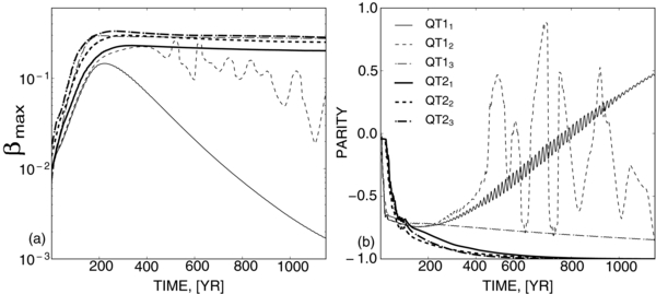
Figure 2. Panel (a) shows the maxima of the toroidal magnetic field strength (normalized to the energy of the turbulent motions) and panel (b) shows the parity indexes evolution in the models. We employ the running average to filter out the separate cycles.
Download figure:
Standard image High-resolution imageThe QT2-type models have no CQ issue. All the evolutionary paths in models QT11, 2, 3 are very similar. The saturation level in the model is βmax ⩽ 0.4.
The difference in the evolution of the magnetic helicity in the models with QT1 and QT2 has been recently discussed by Hubbard & Brandenburg (2012). Taking into account the dynamo equation (4), the corresponding equation for the large-scale vector potential
where we assume the Coulomb gauge (the integral of  over the domain is zero), we find the equation that governs the large-scale helicity evolution:
Therefore, Equation (3) can be rewritten in the form of Equation (2):
The term  consists of the counterparts of the sources' magnetic helicity, which are represented by
  , and the fluxes which result from pumping of the large-scale magnetic fields. The sources' magnetic helicity in the term
  is partly compensated for in Equation (13) by the counterparts in
  . This results in the spatially homogeneous quenching of the large-scale magnetic generation and the alleviation of the CQ problem.
Figure 3 shows snapshots of the magnetic field and magnetic helicity (large- and small-scale) evolution in the north segment of the solar convection zone for model QT21. We observe the drift of the dynamo waves related to the evolution of the large-scale toroidal and poloidal fields toward the equator and toward the pole, respectively. The distributions of the large- and small-scale magnetic helicities show the correspondence in sign: positive to negative, and the other way around, respectively. This agrees with Equation (3). It can be observed that the negative sign of the magnetic helicity follows the dynamo wave of the toroidal magnetic field. This can be related to the so-called current helicity hemispheric sign rule (negative/positive sign of helicity dominate in the north/south hemisphere) which is suggested by the observations (see Seehafer 1990; Zhang et al. 2010, and references therein). The origin of the helicity sign rule has been extensively studied in the dynamo theory (e.g., Choudhuri et al. 2004; Kuzanyan et al. 2006; Sokoloff et al. 2006; Pevtsov & Longcope 2007; Pipin & Kosovichev 2011b; Zhang et al. 2012). Similar snapshots for the QT13 model are shown in Figure 4 (see Figure 5(c) in Pipin & Kosovichev 2011b). The main difference is that for the QT1 model, the magnetic helicity evolution does not follow the dynamo wave inside the convection zone as is demonstrated for the QT2 model. This is further illustrated by Figure 5, which shows variations of the radial profiles of the α-effect and magnetic helicity with the cycle. For all of the models, the changes in the α-effect are concentrated to the top of the convection zone. This is due to the factor  relating the α-effect and the magnetic helicities.
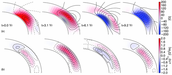
Figure 3. Snapshots of the magnetic field and helicity evolution inside the north segment of the convection zone for model QT21. Panel (a) shows the field lines of the poloidal component of the mean magnetic field and the toroidal magnetic field (varies in the range of ±1 kG) by the background images. Panel (b) shows the large-scale (background images) and small-scale magnetic helicity (contours) distributions. Both kinds of magnetic helicity vary in the same range of magnitude.
Download figure:
Standard image High-resolution image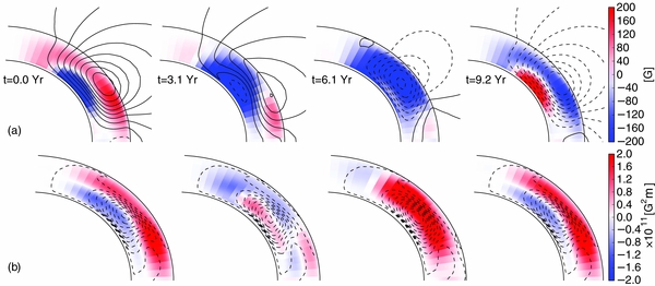
Figure 4. Same as Figure 3 for model QT13.
Download figure:
Standard image High-resolution image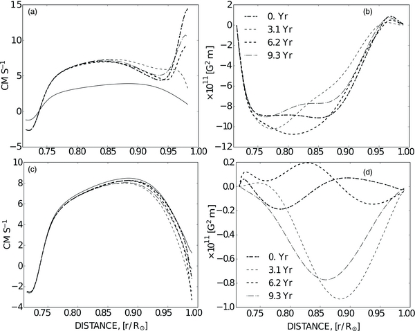
Figure 5. Panels (a) and (b) show variations of the radial profiles for the α-effect (αϕϕ component) and magnetic helicity with the cycle at colatitude θ = 45°, for model QT13. Panels (c) and (d) show the same for model QT21. The solid lines show the original distribution of the α-effect (without dynamical quenching).
Download figure:
Standard image High-resolution imageThe results for models QT13 and QT21 are different despite having the same boundary conditions. Moreover, the QT2-type models can produce the dynamical α-effect as in model QT13 for the different boundary conditions for the magnetic helicity at the top (Pipin 2013). Figure 5(b) shows that for model QT1, the small-scale magnetic helicity remains negative in the bulk of the convection zone, demonstrating the steady wave in the northern hemisphere. For model QT21, we observe the propagation of the helicity wave from the bottom to the top of the convection zone. This propagation is due to the local balance of the large-scale and small-scale helicities.
Model QT21 shows the possibility of the negative dynamical α-effect near the top of the convection zone. Our model employs the subsurface rotational shear, which has the negative radial gradient of the angular velocity. Therefore, the negative dynamical α-effect near the surface prevents penetration of the dynamo wave very close to the equator because of the Parker–Yoshimura rule (Parker 1955; Yoshimura 1975). We note that the negative dynamical α-effect in our model works in a way which is the opposite of the results of the numerical simulation presented by Käpylä et al. (2012), where they have the positive radial gradient of the angular velocity near the surface.
Figure 6 shows the time–latitude and the time–radius diagrams for the large-scale toroidal and poloidal magnetic fields and for the current helicity for model QT21. The helicity patterns change the sign at the edges of the wings of the time–latitude "butterfly" diagrams for the toroidal magnetic field. This roughly agrees with the available observations. The model demonstrates that in the northern hemisphere, the wave with the positive sign of the magnetic helicity propagates from the bottom of the convection zone to the top. Similar results were found in the numerical simulation (Warnecke et al. 2011). This propagation is related to the dynamo wave and not to the mean flow.

Figure 6. Panel (a) shows the time–latitude variations of the toroidal field near the surface, r = 0.95 R☉ (contours are between extreme of ±300G) and the radial magnetic field at the surface (background image) for model QT21; panel (b) shows the same for the toroidal field and the current helicity (background image); panel (c) shows the same for the time–radial distance variations at latitude 30°. The time is measured in years counted from an arbitrary instant.
Download figure:
Standard image High-resolution image
4. DISCUSSION
In this paper, we studied the effect of magnetic helicity conservation in the mean-field solar dynamo model which is shaped by the subsurface shear. Two formulations for the magnetic helicity conservation are examined: one of them is deduced from a consideration of the induction equation for the fluctuating magnetic field and its vector potential. Another formulation is deduced from the integral conservation of the total magnetic helicity. For the first time, we show that the solar dynamo can operate in a wide range of the magnetic Reynolds numbers up to 106 if conservation of the total magnetic helicity is taken into account. We confirmed that the models that employ the first framework (QT1 type models) for the magnetic helicity conservation suffer from CQ unless they use the low Rm or high-turbulent diffusive fluxes. Yet the QT1 models show very different results for the evolution of the magnetic helicity inside the convection zone compared to the models which are based on the conservation of the total magnetic helicity.
The difference in the two frameworks was realized by Hubbard & Brandenburg (2012), who pointed out that the term  is needed in Equation (1) for the conservation of the total magnetic helicity. This term consists of the counterparts of the sources' magnetic helicity and also the helicity fluxes. We showed that the results for models QT1 and QT2 are very different, despite having the same boundary conditions and the same dynamo effects. The most important qualitative difference is that in the QT2-type models, there is a magnetic helicity wave propagating with the dynamo wave from the bottom of the convection zone to the surface. This was clearly demonstrated by Figures 3, 4, and 6. We should note that the total helicity (as the integral over the volume) is conserved in both the QT1 and QT2 models. Compared with the QT1 models, the QT2 models show the local conservation of the magnetic helicity (see Figures 3 and 4). The latter is not valid for the QT1 models. The theoretical details of the processes of the transfer of magnetic helicity over the scales are hidden in the term describing the generation of the large-scale magnetic helicity; see Equations (3) and (12). These details, perhaps, can be restored in direct numerical simulations (e.g., Warnecke et al. 2011). We can use the observations of the small- and large-scale magnetic helicities to test the developed models.
In our paper, we studied the distributed mean-field solar dynamo model operating in the bulk of the convection zone. The models demonstrate two maxima of the radial distribution of the toroidal magnetic field strength: one of them at the bottom and another near the top of the solar convection zone. This is in agreement with the numerical simulations (Brown et al. 2011; Miesch et al. 2011; Racine et al. 2011). The model does not include the effect of meridional circulation which is considered to be the primary mechanism for the transport of the large-scale magnetic field in the Babcock–Leighton-type models (Choudhuri et al. 1995; Dikpati & Charbonneau 1999; Dikpati et al. 2004). We should note that the current observations and the direct numerical simulations do not allow us to choose the particular type among the solar dynamo models. Critical reviews on the solar dynamo can be found in the literature (e.g., Brandenburg 2005; Tobias & Weiss 2007; Charbonneau 2011). The effect of meridional circulation can be very important for magnetic helicity transport in the case of the high Rm. It is expected that for this case, the circulation will define the magnetic helicity distribution. This question needs to be studied separately.
Summarizing our findings, we can conclude that the conservation of magnetic helicity is important for helicity transport from the bottom of the convection zone to the surface. We show that if the total helicity balance is taken into account, then the magnetic helicity propagates with the dynamo wave. This prevents CQ by using a more adequate formulation of the local balance of magnetic helicity. The results we have obtained need further development as many details of the dynamo processes are obscured.
V.P., D.S., and K.K. acknowledge support from the Visiting Professorship Programme of Chinese Academy or Sciences 2009J2-12 and thank the NAOC of CAS for hospitality, and also acknowledge support from the NNSF of China and RFBR of Russia under grant 13-02-91158 and RFBR grants 12-02-00170-a, the support of the Integration Project of SB RAS N 34, and support of the state contracts 02.740.11.0576, 16.518.11.7065 of the Ministry of Education and Science of Russian Federation. H.Z. acknowledges support from National Natural Science Foundation of China grants 41174153, 10921303, and 11221063.