


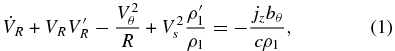
ABSTRACT
A 2.5D, time-dependent magnetohydrodynamic model is used to test the proposition that observed type II spicule velocities can be generated by a Lorentz force under chromospheric conditions. It is found that current densities localized on observed space and time scales of type II spicules and that generate maximum magnetic field strengths ⩽50 G can generate a Lorentz force that accelerates plasma to terminal velocities similar to those of type II spicules. Maximum vertical flow speeds are ∼150–460 km s−1, horizontally localized within ∼2.5–10 km from the vertical axis of the spicule, and comparable to slow solar wind speeds, suggesting that significant solar wind acceleration occurs in type II spicules. Horizontal speeds are ∼20 times smaller than vertical speeds. Terminal velocity is reached ∼100 s after acceleration begins. The increase in the mechanical and thermal energy of the plasma during acceleration is (2–3) × 1022 ergs. The radial component of the Lorentz force compresses the plasma during the acceleration process by factors as large as ∼100. The Joule heating flux generated during this process is essentially due to proton Pedersen current dissipation and can be ∼0.1–3.7 times the heating flux of ∼106 ergs cm−2 s−1 associated with middle-upper chromospheric emission. About 84%–94% of the magnetic energy that accelerates and heats the spicules is converted into bulk flow kinetic energy.
Export citation and abstract BibTeX RIS
1. INTRODUCTION
Type II spicules are a recently discovered phenomenon. They appear to be upward jets of heated plasma in the chromosphere. They were first observed at the limb (De Pontieu et al. 2007a, 2007b, 2007c) and later identified with so-called rapid blueshifted excursions (RBEs) on the disk (Langangen et al. 2008; Rouppe van der Voort et al. 2009; Sekse et al. 2012). They extend over height ranges ∼103 km; have maximum vertical flow speeds ∼50–150 km s−1, durations ∼10–150 s, are characteristic diameters ≲ 200 km; are heated to transition region temperatures during their acceleration; and exhibit horizontal motions, sometimes inferred to be due to superimposed Alfvén waves, with speeds ∼5–10 times less than the maximum vertical speeds.
Maximum vertical flow speeds of ∼50–150 km s−1 are inferred for type II spicules from limb observations (De Pontieu et al. 2007a, 2007b, 2007c). Maximum vertical flow speeds of ∼20–70 km s−1 (Rouppe van der Voort et al. 2009) and ∼10–50 km s−1 (Sekse et al. 2012) are inferred for RBEs from disk observations. The smaller values of the speeds inferred from the disk observations are probably due to a combination of projection effects on the disk that tend to reduce the apparent upward speed, the fact that limb observations are biased toward detecting those type II spicules that extend farthest above the limb and so tend to have the largest upward speeds, and the tendency of the on-disk velocity observations to sample lower heights in the atmosphere where speeds tend to be smaller (Rouppe van der Voort et al. 2009).
It is speculated that type II spicules are a major source of mass and energy for the corona (De Pontieu et al. 2009, 2011). Their acceleration and heating mechanisms are unknown.
There is an opposing view that RBEs are not type II spicules and that type II spicules are not jets of plasma but instead are warping, mainly vertical, two-dimensional sheets of magnetic field lines (Judge et al. 2011). The first part of this view is based on comparing the estimate of the occurrence rate of type II spicules made by Judge & Carlsson (2010) with the estimate of the occurrence rate of RBEs made by Rouppe van der Voort et al. (2009). Those estimates suggest that type II spicules occur ∼10–100 times more frequently than RBEs. Doppler shift measurements from the upcoming IRIS mission1 are expected to contribute to resolving this controversy.
In the magnetohydrodynamic (MHD) model of a plasma, the acceleration of bulk flow is driven by the pressure gradient and Lorentz forces. The purpose of this paper is to use a 2.5D, time-dependent MHD model to determine if the Lorentz force generated by a horizontally localized current density of finite duration can accelerate vertical flows to speeds characteristic of type II spicules within their observed lifetimes and horizontal diameters, and within ranges of density, temperature, and magnetic field strength believed to be reasonable for the middle-upper chromosphere.
Solutions to the model suggest that type II spicules can be driven by this Lorentz force under chromospheric conditions. For these solutions the Joule heating flux, when averaged over horizontal regions with diameters of 50–200 km, reaches values ∼0.1–3.7 times the characteristic time-averaged middle-upper chromospheric radiative loss rate of ∼106 ergs cm−2 s−1 (Anderson & Athay 1989; Fontenla et al. 2002) for ∼10–20 s before decreasing back to background values.
2. THE MODEL
The strategy is to consider a model that can be solved with high accuracy to avoid significant numerical error and that contains an essential description of a 2.5D bulk flow accelerated by a spatially and temporally localized Lorentz force. This is done by specifying a form for a spatially and temporally localized vertical current density and then deriving the corresponding radial current density, in cylindrical coordinates, under the assumption that the azimuthal current density is zero. The magnetic field is computed from the current density. Additional assumptions then allow the momentum and mass conservation equations to be solved analytically for the velocity, density, and pressure. Although the model is restricted to a specific form of the current density, and hence of the magnetic field, it is proposed that more general current densities with orders of magnitude and spatial and temporal localization scales similar to those used in the model also give rise to Lorentz forces that can accelerate chromospheric plasma to type II spicule velocities. In this sense, the model represents a special case of a more general Lorentz force acceleration mechanism that might play an important role in accelerating type II spicules.
Assume cylindrical coordinates (R, θ, z), and let t be time. All quantities are independent of θ, and z is height above some unspecified point in the middle-upper chromosphere. Assume a weakly ionized H plasma with a constant temperature T. Then p = ρkBT/mp = ρV2s, where p, ρ, Vs, mp, and kB are the pressure, mass density, sound speed, proton mass, and Boltzmann's constant. Assume p = p1(R, t)exp (− z/L) and ρ = ρ1(R, t)exp (− z/L), where L = kBT/mpg is the ideal gas pressure scale height and g = 2.74 × 104 cm s−2.
Let V be the center-of-mass (bulk flow) velocity. Assume the magnetic field B = b(R, t)exp (− z/2L). Neglecting viscous effects in the momentum equation, it follows from the momentum and mass conservation equations that an exact solution for the height dependence of V is that it is independent of height. This form of the solution is assumed here, so V = V(R, t). The assumed form of the height dependence of B, V, and ρ implies that the flow is accelerated by a height-independent Lorentz force per unit mass along a column of gas. The current density J = j(R, t)exp (− z/2L) = c∇ × B/4π. It is assumed that jθ = 0.
Under the preceding assumptions, the momentum and mass conservation equations are


Here the dot and prime denote ∂/∂t and ∂/∂R.
The assumption that T is constant and that p varies with z according to the factor exp (− z/L) causes the gravitational force term −ρg and ∂p/∂z to cancel one another in the vertical component of the momentum equation, which is Equation (3). That is why these terms do not appear in that equation. Then, the vertical pressure gradient and the gravitational force do not play any role in the vertical acceleration of the plasma for the model presented here, although they are both time dependent and increase by orders of magnitude during the acceleration process for the model solutions in Section 4.
Since jθ = 0, it follows that (∇ × B)θ = 0, so BR and Bz together make up a potential field. This equation, together with the constraint ∇ · B = 0, determines this field to be a constant vertical field B0 plus a radial and additional vertical component given by br = b0J1(R/2L) and bz = b0J0(R/2L), where J0, 1 are Bessel functions of the first kind of order 0 and 1. Here, b0 is chosen to be zero for simplicity. Then, BR = 0 and Bz = B0.
Type II spicule velocities are mainly vertical and appear to be parallel to a guide magnetic field, but they can have a significant component perpendicular to this main flow. Sekse et al. (2012) observe horizontal motions of RBEs with speeds mainly ∼5–10 km s−1, with most peak speeds ∼5 km s−1 and maximum speeds ∼20 km s−1. These horizontal motions are superimposed on vertical flows with apparent speeds ∼10–50 km s−1, noting that the actual vertical flow speeds may be significantly higher due to projection effects. De Pontieu et al. (2012) observe torsional and swaying motions of type II spicules on the limb with speeds ∼25–30 and 15–20 km s−1 that are perpendicular to and superimposed on nearly vertical flows (∼20° inclination) with speeds ∼50–100 km s−1. De Pontieu et al. (2012) conjecture that these transverse, mainly horizontal motions are due to Alfvén waves with periods ∼100–300 s that propagate along the spicules. Since these periods are ≳ spicule lifetimes (∼100 s), it is difficult or impossible to observe a complete oscillation. It is expected that Alfvén waves occur in type II spicules because these waves are one of the fundamental MHD wave modes that must be continually excited in a magnetized atmosphere driven by convection with a wide range of temporal and spatial scales. It is not known if these waves play an important role in accelerating or heating type II spicules.
The model used here does not model waves, and although the model solutions have horizontal flows, these flows are restricted to be sufficiently small in magnitude to simplify solving the model for the vertical flow speed. This restriction is consistent with the observation that the primary acceleration is in the vertical direction, but it results in the model generating horizontal flow speeds that are not as large a fraction of the vertical flow speeds as suggested by the observations of Sekse et al. (2012) and De Pontieu et al. (2012). The horizontal flow speeds in the model are restricted in the following way. Constraints are imposed on VR to justify omitting the terms involving VR in the momentum Equations (1)–(3). Inspection of these equations indicates that the constraints |VR| ≪ |Vz| and |VR| < Vs should be adequate. The additional constraint  allows the V2θ/R term in Equation (1) to be omitted in first approximation. Here
  , where R0 is the radial scale of the current density, defined in Section 2.1. As shown in Section 3, the constraint on VR places an upper bound on R0, and the constraint on Vθ places an upper bound on B0.
Despite the neglect of wave motion and the upper bounds placed on the horizontal flow speeds, the model solutions show that the vertical flow speed can be accelerated to type II spicule values, with maximum speeds comparable to slow solar wind speeds (∼ 200–400 km s−1) on sub-resolution horizontal spatial scales. This suggests that the primary acceleration mechanism of type II spicules does not involve waves with periods ≲ type II spicule lifetimes, consistent with the observations and conjecture of De Pontieu et al. (2012) discussed above.
After applying the constraints on the horizontal flow speeds indicated above, the radial component of the momentum equation, which is Equation (1), states that ∂p/∂R balances the radial Lorentz force. This gives rise to radial compression of the plasma. This is a z pinch effect since the radial Lorentz force is generated by Jz and Bθ.
2.1. Current Density and Azimuthal Magnetic Field
The vertical current density jz is assumed to be localized in time and space with characteristic time and radial scales t0 and R0 and to have the following functional form:

Here  and
and  .
.
It follows from ∇ · j = 0 that the radial current density
From ∇ × B = 4πJ/c, it follows that
where bθ0 ≡ 2πj0R0/c. A plot of bθ/bθ0 is shown in Figure 1.

Figure 1. Normalized azimuthal magnetic field at selected times.
Download figure:
Standard image High-resolution imageWith respect to  , the maximum values of jz, jr, and bθ are reached at
  , for which
 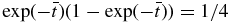 . With respect to
  , the maximum values of jr and bθ are reached at
  , for which
 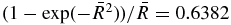 . The maximum value of bθ and hence of Bθ is then 0.6382 bθ0/4 = 0.1596 bθ0. Then specifying bθ0 determines the maximum magnitude of the magnetic field and determines j0R0.
3. GENERAL SOLUTION
Omit the terms involving VR in Equations (1)–(3), and omit the term involving Vθ in Equation (1), assuming the constraints on VR and Vθ discussed in Section 2. Solving these equations successively for ρ1, Vθ, and Vz gives
where
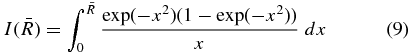
and Imax = I(∞) = 0.3466.  reaches 99% of Imax at
  ,
,
where

Then, solving Equation (4) for VR gives
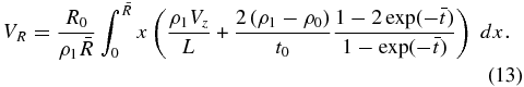
ρ1, Vz, and Vθ depend on R only through  , and in this sense they are scale invariant. VR explicitly involves a factor of R0, so the profile of VR scales linearly with R0. This is where the constraint on R0 enters the solution. For given values of the other input parameters, R0 must be chosen sufficiently small so that |VR| ≪ |Vz| and |VR| < Vs. Only Vθ involves B0. For given values of the other input parameters, B0 must be chosen sufficiently small so that
  .
.
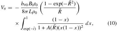
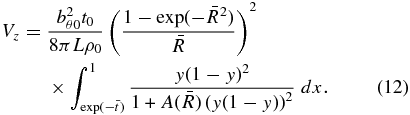
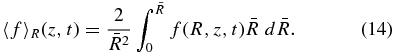
The average of any quantity f(R, z, t) over the horizontal circular area πR2 centered at R = 0 is denoted by 〈f〉R and is computed as
Equation (12) shows that Vz increases with  to a finite, terminal,
  -dependent speed determined by the inputs to the model. As
  , Equation (8) shows that
  . It follows from Equation (13) that the terminal profile for VR is
For the particular solutions presented in Section 4, the terminal velocity profile is essentially reached for  .
.
4. PARTICULAR SOLUTIONS
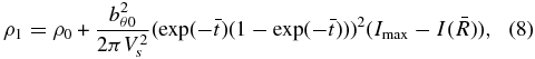
The acceleration is assumed to occur in the middle-upper chromosphere. The inputs to the model are R0, t0, bθ0, ρ0, and T0. Two solutions are presented. For both solutions t0 = 33.3 s, T0 = 7000 K, B0 = 0.5 G, and ρ0 ≡ mpn0, where n0 = 1012 cm−3. Then Vs = 7.6 km s−1 and L = 211 km. The choice of such a small value of B0 is necessary to satisfy the constraint on Vθ discussed in Section 3 and is probably an artifact of the simplicity of the model. All plots in Sections 4.1 and 4.2 are at the reference height z = 0, except as otherwise indicated.
4.1. Solution 1
For this solution, R0 = 5 km and bθ0 = 156.7 G. Then, Bθ ⩽ 25 G and j0 = 4.984 A m−2. Figures 2– 8 show radial profiles of the solution for selected times.

Figure 2. Number density at selected times. R0 = 5 km.
Download figure:
Standard image High-resolution image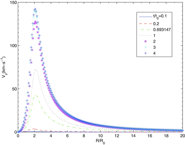
Figure 3. Vertical velocity at selected times. R0 = 5 km.
Download figure:
Standard image High-resolution image
Figure 4. Radial velocity at selected times. R0 = 5 km.
Download figure:
Standard image High-resolution image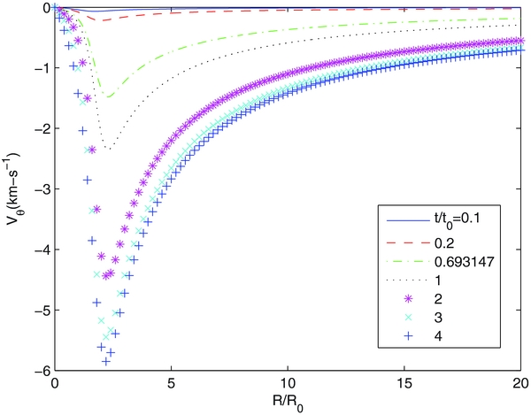
Figure 5. Azimuthal velocity at selected times. R0 = 5 km.
Download figure:
Standard image High-resolution image
Figure 6. Terminal profiles of the radial average of the vertical velocity, together with the radial, azimuthal, and horizontal velocities. R0 = 5 km.
Download figure:
Standard image High-resolution image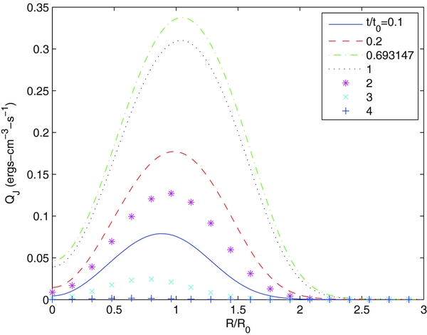
Figure 7. Joule heating rate per unit volume at selected times. R0 = 5 km.
Download figure:
Standard image High-resolution image
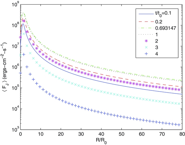
Figure 8. Radial average of the Joule heating flux at selected times. R0 = 5 km.
Download figure:
Standard image High-resolution imageFigure 2 shows the number density n = ρ/mp. During the acceleration process, the plasma is compressed to a density ∼100 times its pre-acceleration value. Maximum compression is on the axis, and the region of significantly increased density has a diameter of ∼20 km. Maximum compression is reached at t ∼ 0.693t0 = 23 s, and the density returns to its pre-acceleration value after a duration of ∼4t0 = 133 s.
Figure 3 shows the vertical velocity Vz. The plot extends to  , corresponding to R = 100 km, and hence to a diameter of 200 km. The terminal velocity profile is reached at t ∼ 3t0 = 100 s. The maximum of Vz = 142.4 km s−1 and occurs at R = 10.5 km. Vz < Vs for R > 50 km.
Figures 4 and 5 show VR and Vθ. They are ≪Vz almost everywhere, in particular in the region where Vz is near its maximum value. Then V is essentially vertical. Figure 4 shows that at early times VR < 0 and that VR rapidly increases to positive values for later times.
Figure 6 shows 〈Vz〉R, VR, Vθ, and the horizontal flow speed VH = (V2R + V2θ)1/2 at t = 4t0, after the acceleration is over. The figure suggests that if an observation effectively averages the vertical velocity over diameters ∼50, 100, or 200 km, the inferred terminal vertical flow speeds are ∼66, 27, and 10 km s−1.
4.1.1. Joule Heating Rate
The standard expression for the Joule heating rate per unit volume due to the Spitzer resistivity η and the magnetization-induced Pedersen resistivity ηΓ is (e.g., Mitchner & Kruger 1973)

where J⊥ is the component of J⊥B. The magnetization factor Γ = MeMp(ρn/ρ)2, where Me, Mp, and ρn are the electron and proton magnetizations and the neutral density, respectively. In the chromosphere ρn ∼ ρ. Explicitly,


Here me, ne, e, and σ(= 5 × 10⁻¹⁵ cm2) are the electron mass, density, and charge magnitude and the charged-neutral particle scattering cross section, respectively (Osterbrock 1961).2 All quantities in Equations (17)–(19) are known except ne.
An approximate expression for ne under solar chromospheric conditions is derived in Goodman & Judge (2012). It is

Here T2 = 1.18187 × 10⁵ K, α = 3.373 × 10⁻¹³, b = −0.786, and nH is the H i density. Equation (20) includes all lowest order non-LTE (NLTE) effects. In the present model, nH = ρ/mp. Equation (20) with T = T0 is used here to estimate QJ. The heating flux FJ ∼ ∫∞0QJ dz ∼ 2LQJ(R, t).
Figure 7 shows QJ. Joule heating is confined within a radius of 10 km. The Pedersen current dissipation rate ΓηJ2⊥ is ∼102–103 times larger than the Spitzer heating rate ηJ2. This is due to the large magnetization-induced resistivity Γη ≫ η. Since QJ(R, z, t) ∼ exp (− z/2L)QJ(R, t), where 2L = 422 km, QJ decreases by a factor of 10 over a height range of 103 km.
Figure 8 shows 〈FJ〉R. The figure shows that the maximum value 〈FJ〉R over diameters of 50, 100, and 200 km is ∼(13, 3, 1) × 105 ergs cm−2 s−1, respectively, to be compared with the observed middle-upper chromospheric heating rate of ∼106 ergs cm−2 s−1. This suggests that the resistive heating rate in type II spicules can exceed that in the surrounding plasma by ∼10%–100% for ∼10–20 s.
4.2. Solution 2
This solution explores the effect of increasing the maximum value of Bθ by a factor of 2 to 50 G. Then R0 must be reduced by a factor of 4 to 1.25 km to keep |VR| sufficiently small. Then, bθ0 = 313.4 G and j0 = 39.875 A m−2, which is a factor of 8 larger than for Solution 1.
Equation (8) shows that the maximum density increases by a factor of ∼4 over that of Solution 1, to ∼(3–4) × 1014 cm−3. The region of significantly increased density has a diameter of ∼5 km.
Figure 9 shows Vz. As before, the terminal velocity profile is reached at t ∼ 3t0 = 100 s. The maximum of Vz = 456.3 km s−1, which is comparable to the slow solar wind speed and occurs at R = 3 km. Vz < Vs for R > 25 km.
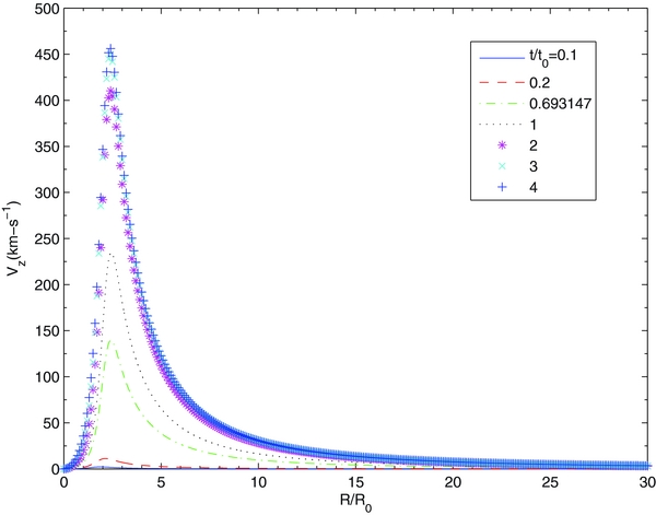
Figure 9. Vertical velocity at selected times. R0 = 1.25 km.
Download figure:
Standard image High-resolution imageFigure 10 shows 〈Vz〉R, VR, Vθ, and VH at t = 4t0. The figure suggests that if an observation effectively averages the vertical velocity over diameters of ∼50, 100, and 200 km, the inferred terminal vertical flow speeds are ∼35.5, 11.6, and 3.6 km s−1, respectively. These vertical speeds are ∼2–3 times smaller than those for Solution 1, even though the maximum vertical flow speed is 3.2 times larger than for that solution. This is because the current density, and hence the acceleration, is confined within a smaller radius.
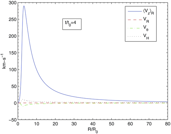
Figure 10. Terminal profiles of the radial average of the vertical velocity, together with the radial, azimuthal, and horizontal velocities. R0 = 1.25 km.
Download figure:
Standard image High-resolution imageBoth solutions have an annular region defined by  in which the vertical flow speed is highly supersonic, with maximum values comparable to slow solar wind speeds. Since the thickness of these regions is ∼5–20 km, relatively high resolution is needed to resolve them if they exist. One test of the viability of the acceleration mechanism modeled here is to see if future, higher resolution observations reveal overall higher flow speeds as the region of maximum flow speed predicted by the model is increasingly better resolved.
Figure 11 shows QJ. It is ∼35 times larger than QJ for Solution 1.
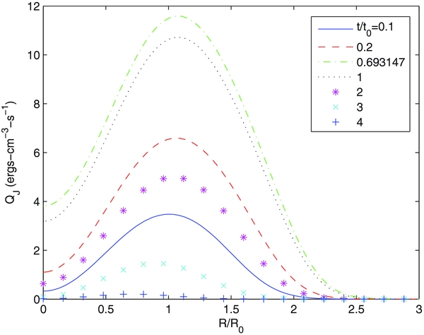
Figure 11. Joule heating rate per unit volume at selected times. R0 = 1.25 km.
Download figure:
Standard image High-resolution imageFigure 12 shows 〈FJ〉R. The figure shows that 〈FJ〉R over diameters of 50, 100, and 200 km is ∼(36.8, 9.2, 2.3) × 105 ergs cm−2 s−1, respectively. Similar to the corresponding result for Solution 1 shown in Figure 8, this suggests that the resistive heating rate in type II spicules can exceed that in the surrounding plasma by ∼23%–368% for ∼10–20 s.
Figure 12. Radial average of the Joule heating flux at selected times. R0 = 1.25 km.
Download figure:
Standard image High-resolution image
The result for Solutions 1 and 2 that Vz reaches maximum speeds ∼150 and 460 km s−1 over radially localized regions with sub-resolution diameters suggests that significant slow solar wind acceleration occurs in type II spicules on sub-resolution horizontal spatial scales.
5. ENERGY INPUT
The magnetic energy before and after the acceleration is the same. Then Poynting's theorem implies that all the energy for accelerating and heating the plasma flows into the acceleration region as a Poynting flux and is entirely converted into thermal and bulk flow kinetic energy. Explicitly, Poynting's theorem implies ∫∞0(QJ + V · (J × B)/c) dt = −∫∞0∇ · S dt, where S is the Poynting flux. Then, the integral of QJ + V · (J × B)/c over time and volume gives the total energy input into the plasma as the sum of the thermal energy input EJ and the work W done in accelerating the plasma. These quantities are estimated as follows:


For Solutions 1 and 2, let  and 80, corresponding to a diameter of 200 km. For Solution 1, W = 2.36 × 10²² ergs and EJ = 1.35 × 10²¹ ergs, so the total energy input is 2.5 × 10²² ergs. About 94.4% of this energy is converted into bulk flow kinetic energy. For Solution 2, W = 1.93 × 10²² ergs and EJ = 3.81 × 10²¹ ergs, so the total energy input is 2.31 × 10²² ergs. About 84% of this energy is converted into bulk flow kinetic energy. Almost all of the electromagnetic energy that heats and accelerates the plasma is converted into bulk flow kinetic energy. The total energy inputs for Solutions 1 and 2 are ∼5 times smaller than characteristic nanoflare energies of ∼1023–1024 ergs.3
6. CONCLUSIONS
Current densities localized on space and time scales of type II spicules and that generate reasonable magnetic field strengths can give rise to a Lorentz force that accelerates chromospheric plasma to terminal vertical and horizontal velocities similar to those of type II spicules. A vertical pressure gradient is not needed to generate the observed flows, although in reality it might play an important role in spicule acceleration.
The maximum vertical flow speeds occur in horizontally localized regions with sub-resolution diameters near the axis of the spicules. These speeds can reach values comparable to slow solar wind speeds ∼150–460 km s−1. This suggests that the acceleration of type II spicules is an important part of the mechanism that accelerates the slow solar wind.
Almost all of the magnetic energy that accelerates and heats the plasma is converted into bulk flow kinetic energy, as opposed to thermal energy.
The radial component of the Lorentz force compresses the plasma during the acceleration process, possibly by factors as large as ∼100, although the highest densities remain within the known chromospheric density range. The Joule heating flux generated during the acceleration process is essentially entirely due to proton Pedersen current dissipation, and it can be a significant fraction of and may exceed the heating flux of ∼106 ergs cm−2 s−1 associated with the relatively quasi-steady middle-upper chromospheric emission.
In the model used here, the Joule heating rate is uncoupled from the predicted V, ρ, and p in that it has no effect in determining these quantities. This is a result of the model not including an energy equation, which is redundant given the assumption of constant T. If this assumption is relaxed, an energy equation must be included in the model, which then self-consistently determines T along with V, ρ, and p. Such a model can use the approximate analytic expressions for the NLTE ionization fraction and radiative cooling rate in the chromosphere derived in Goodman & Judge (2012), in which case the electron density and radiative cooling rate are also computed self-consistently by the model.
A model that self-consistently includes an energy equation, variable T, realistic transport coefficients (most importantly the electrical conductivity tensor for a partially ionized plasma), and NLTE ionization and radiative cooling and that is solved with sufficient numerical resolution to resolve the smallest relevant length scales is needed to accurately model energy flow and transformation rates, including radiative emission. No such model exists. The smallest length scales that must be resolved to accurately describe type II spicule heating and acceleration are unknown, although the results presented here suggest that a horizontal resolution ≲ 5 km is necessary.
If magnetic reconnection plays a role in type II spicule formation, then the radiating current sheet solutions in Goodman & Judge (2012) might give an indication of the resolution needed to resolve the resistive length scales in the chromosphere. These solutions indicate that a numerical resolution ≲ 10–100 m is needed, aside from it being necessary to ensure that any artificial diffusive effects introduced into the model are much smaller than the physical diffusive effects described by the realistic transport coefficients in the model. The fact that the ionization fraction and radiative emission rates are exponentially sensitive functions of T, and that T is largely determined by diffusive transport processes such as Joule heating, emphasizes the need to use realistic transport coefficients and fully resolve their effects.
The origin of the current density in the model used here is not indicated. Processes that generate this current density, or more generally that generate a Lorentz force similar to the one modeled here, need to be identified. Magnetic reconnection might be such a process. Other processes must also be considered, such as that suggested by the simulations of Martínez-Sykora et al. (2011), which involves horizontal compression by a Lorentz force causing a vertical pressure gradient that accelerates plasma along a mainly vertical magnetic field. This horizontal compression and the radial compression in the model solutions presented here might cause a transient compressive heating rate −p∇ · V that causes an observable increase in radiative emission.
The author gratefully acknowledges support from grants ATM-0650443 and ATM-0848040 from the Solar Physics Program of the National Science Foundation to the West Virginia High Technology Consortium Foundation. The author thanks the referee for constructive remarks that led to significant improvements in the paper. This research made use of NASA's Astrophysics Data System (ADS).
Footnotes
- 1
- 2
σ includes charge exchange effects.
- 3
Nanoflares are magnetic reconnection events that convert ∼1023–1024 ergs of magnetic field energy into wave and particle kinetic energy. The prefix "nano" derives from this amount of energy being ∼10−9 times the energy of a large flare, which is ∼1032–1033 ergs.