


ABSTRACT
We present simulations of coronal mass ejections (CMEs) performed with a new two-temperature coronal model developed at the University of Michigan, which is able to address the coupled thermodynamics of the electron and proton populations in the context of a single fluid. This model employs heat conduction for electrons, constant adiabatic index (γ = 5/3), and includes Alfvén wave pressure to accelerate the solar wind. The Wang–Sheeley–Arge empirical model is used to determine the Alfvén wave pressure necessary to produce the observed bimodal solar wind speed. The Alfvén waves are dissipated as they propagate from the Sun and heat protons on open magnetic field lines to temperatures above 2 MK. The model is driven by empirical boundary conditions that includes GONG magnetogram data to calculate the coronal field, and STEREO/EUVI observations to specify the density and temperature at the coronal boundary by the Differential Emission Measure Tomography method. With this model, we simulate the propagation of fast CMEs and study the thermodynamics of CME-driven shocks. Since the thermal speed of the electrons greatly exceeds the speed of the CME, only protons are directly heated by the shock. Coulomb collisions low in the corona couple the protons and electrons allowing heat exchange between the two species. However, the coupling is so brief that the electrons never achieve more than 10% of the maximum temperature of the protons. We find that heat is able to conduct on open magnetic field lines and rapidly propagates ahead of the CME to form a shock precursor of hot electrons.
Export citation and abstract BibTeX RIS
1. INTRODUCTION
Coronal mass ejections (CMEs) are a manifestation of solar magnetic eruptions, which are seen in coronagraph images as billions of tons of plasma are expelled into interplanetary space with speeds covering a range from less than 100 km s−1 to those exceeding 3000 km s−1. At speeds above 1000 km s−1, CMEs drive shock waves through the corona, which have been directly observed (see, for example, Sime & Hundhausen 1987; Mancuso et al. 2002; Vourlidas et al. 2003; Ontiveros & Vourlidas 2009). The environment in which these shock waves pass is extremely complex as the plasma is heated to more than 1 MK by a wide range of wave–particle and particle–particle interactions that dampen waves and dissipate time varying electric currents. Hydrogen is fully ionized, and all other atomic species are highly ionized. The electron and proton populations are far from thermal equilibrium, the full complexity of which can only be described by kinetic models with non-Maxwellian velocity distribution functions (Landi & Pantellini 2003). For electrons, there are two nearly isotropic populations: the thermal core and the suprathermal halo, and a field-aligned strahl component (Rosenbauer et al. 1977) that travels away from the Sun. Ions are more often characterized by a population that is anisotropic with a temperature perpendicular to the magnetic field higher than that parallel to field.
The purpose of this paper is to present and understand simulations which describe the temporal-spatial variation in temperature that occurs for both proton and electron populations with the passage of CME-driven shock waves. The fundamental issue at hand is that protons are almost 2000 times more massive than electrons so that at 1 MK their respective sound speeds are 120 km s−1 and 5100 km s−1. The speed of fast CMEs falls between these values where they shock the protons but not the electrons. Furthermore, beyond a distance of two solar radii (Rs), collisions become so infrequent that protons and electrons thermally decouple on the timescale of the shock passage. Farther from the Sun, protons will continue to be heated by the CME-driven shock while electrons will begin to cool from adiabatic expansion and heat conduction.
An examination of both particle species with electron heat conduction has been performed with one-dimensional two-temperature simulations of coronal shocks (Kosovichev & Stepanova 1991; Stepanova & Kosovichev 2000). We follow this work with a global multi-dimensional CME model with realistic coronal field geometry. CMEs have typically been simulated with single-fluid three-dimensional (3D) magnetohydrodynamical (MHD) models that address only the thermodynamics of the ion species, and assume that the electrons must be of the same temperature. The thermodynamics of the corona for these models have been addressed with empirical heating functions (Groth et al. 2000) or a variable adiabatic index (Wu et al. 1999; Roussev et al. 2003b; Cohen et al. 2007). An examination of the temperature structure resulting from a CME-driven shock simulated with the coronal model of Groth et al. (2000) is found in Manchester et al. (2004). In this single-fluid model, electron and proton temperatures are assumed equal, which are summed and dynamically treated with a single total temperature. This total (plasma) temperature reaches a value of 2.0 × 10⁷ K behind the CME-driven shock traveling at 900 km s−1 at a distance of 8 Rs. More sophisticated global 3D single-fluid models have followed that treat heat conduction and radiative losses, which together allow the model to be extended to the chromosphere (Lionello et al. 2009; Downs et al. 2010). CMEs have been simulated with the coronal model of Downs et al. (2010), which applies electron heat conduction to the ion fluid. This simulation successfully reproduces images of the low corona as found by the Extreme UltraViolet Imagers (EUVIs) on the Solar Terrestrial Relations Observatory (STEREO) spacecraft.
There are more sophisticated one-dimensional treatments of the solar corona (e.g., Tu & Marsch 1997; Laitinen et al. 2003; Vainio et al. 2003; Suzuki 2006; Cranmer 2010) that include advanced treatment of Alfvén waves, heat conduction, and radiation. For our CME simulations, we make use of a coronal model that addresses the same physical processes in fully 3D geometry, the two-temperature coronal model developed by van der Holst et al. (2010), which describes the coronal plasma as a magnetized proton–electron neutral fluid with a single velocity. The thermodynamics of the two particle populations are treated with two separate energy equations with unique features that are a direct result of the greatly different masses of protons and electrons. Ions are heated by the dissipation of Alfvén wave energy owing to their much lower gyro frequency. Similarly, the proton thermal speed is much lower than that of electrons. Consequently CME-driven shocks exceed the proton sound speed and dissipatively heat the protons, while the same shock is subsonic to the electrons, which are only heated by the adiabatic compression as they pass through the shock. Because of their much higher thermal speed, heat conduction is included only for electrons close to the Sun with the collisional formulation of Spitzer. Finally, the thermal coupling of electrons and protons by particle collisions is addressed with the appropriate heat exchange terms in the energy equations.
In the next section, we describe the numerical model used to perform the simulations, followed by Section 3, which describes the model results. In this paper, we describe two CME simulations with two distinct magnetic field line geometries, one with a CME originating from within the streamer belt surrounded by closed flux and a second originating from an active region with open flux. The purpose of these two distinct simulations is to illustrate the effect that field line geometry has on heat propagation. In Section 4, we present a summary and draw conclusions regarding the simulations.
2. MODEL DESCRIPTION
Here, we briefly summarize the two-temperature coronal model of van der Holst et al. (2010). In this model, the plasma is taken to be fully ionized hydrogen that is magnetized and a perfect conductor of electricity. The transport of the plasma is characterized by a single bulk velocity that applies to both protons and electrons without charge separation. Energy exchange between the species is provided by collisional heat transfer, the rate of which is proportional to the difference in temperatures at a timescale determined by the particle collision rate. The model includes the propagation of Alfvén waves in the WKB approximation in which the wave energy is transported parallel to the magnetic field at the Alfvén speed with the addition of fluid velocity, which may have a component parallel to the magnetic field. The waves provide an isotropic pressure, which, combined with the thermal pressure of the protons and electrons, accelerates the plasma from the Sun to form the solar wind.
As they travel, the Alfvén waves are damped and deposit their energy to the protons. The dissipation rate chosen for our model follows the Kolmogorov power law with the rate proportional to the energy density raised to the power of 3/2. As recent analysis of solar wind turbulence by Li et al. (2011) shows, the Kolmogorov scaling law is applicable to MHD turbulence in the location of current sheets. However, in current-sheet-free locations, the turbulence scaling law of Iroshnikov (1964) and Kraichnan (1965) is obeyed, where turbulent power is proportional to k−3/2 rather than k−5/3, where k is the Alfvén wave number. The difference in damping rates does not have a significant impact on our model, as the damping length has been chosen to produce model results that closely match the observed density, temperature, and velocity of the solar wind (Jin et al. 2012).
Heat conduction is applied only to the electrons with the form of the collisional Spitzer law. We keep the formalism of van der Holst et al. (2010) and prescribe that the heat flux go smoothly to zero beyond a distance of 10 Rs. The cutoff value for the heat conduction at 10 Rs is based on Landi & Pantellini (2003), which presents the results of a 1D kinetic model of the solar wind extending from the base of the corona to interplanetary space. In this model, both electron and proton populations are described with discrete particles that interact through Coulomb collisions. Figure 6 of Landi & Pantellini (2003) shows the kinetic electron heat flux of their model plotted along with the classical Spitzer–Harm heat flux that we employ in our model. Here, very close agreement between the kinetic heat flux and the classical heat flux is found inside of 10 Rs with a growing departure in the heat fluxes beyond this distance. Based on the results of Landi & Pantellini (2003), we do not follow CME evolution beyond a distance of 5 Rs and the heat front beyond a distance of 10 Rs. To go beyond 10 Rs, we need to transition the heat flux to a collisionless form in which the heat flux moves with the electron bulk velocity (Hollweg 1978).
2.1. System of Equations
The two-temperature coronal model is incorporated within the BATS-R-US code, which solves the equations of MHD in conservative form with upwind finite-volume schemes on a Cartesian block-adaptive mesh (Powell et al. 1999; Tóth et al. 2012). This code has previously been used to model both the solar corona (Groth et al. 2000; Roussev et al. 2003b; Cohen et al. 2007; van der Holst et al. 2010) and CMEs (e.g., Groth et al. 2000; Manchester et al. 2004; Roussev et al. 2003a; Tóth et al. 2007; van der Holst et al. 2009), and has recently been greatly advanced for the purpose of simulating high-energy, high-density laser experiments (van der Holst et al. 2011, 2012). The MHD system of equations given below comprises the coronal model (as given in van der Holst et al. 2010) and is solved with the BATS-R-US code:
where ρ is the mass density; u is the velocity; pp, pe, Tp, and Te are the proton and electron pressures and temperatures, respectively; B is the magnetic field; r is the radial distance from the Sun center; G is the gravitational constant; M☉ is the solar mass; and the adiabatic index, γ, is set to a value of 5/3 for an ideal gas. The final equation describes the evolution of the Alfvén waves.  is the Alfvén speed, Ew and pw are the Alfvén wave energy density and pressure, respectively, with pw = Ew/2, and Qp is the wave dissipation. The ± sign for the Alfvén speed applies to two Alfvén wave solutions propagating in opposite directions along magnetic field lines.
The time period of collisional energy exchange is defined by
where e, me, and ne are the electron charge, mass, and number density, mp is the proton mass, and kB and  o are Boltzmann's constant and the permittivity of free space, respectively. Here, we assume that the Coulomb logarithm is spatially uniform with a value of ln Λ = 20. In this formalism, the energy exchange rate between electrons and protons is defined as σie = 2kBnp/τ, where np is proton number density. The electron thermal heat flux follows the collisional formulation of Spitzer:
where κe ≈ 9.2 × 10⁻¹² W m−1 K−7/2, again assuming ln Λ = 20.
BATS-R-US solves the MHD equations in conservative form such that energy dissipated at shocks is transferred only to the proton thermal energy (Powell et al. 1999) to ensure jump conditions are properly maintained. Similarly, energy dissipated at magnetic current sheets is also transferred to the ions, which may then be transferred to electrons via collisions, and in this way mimics Joule heating.
We employ six levels of refinement in a computational domain that extends from −24 Rs < x, y, z < 24 Rs with the lower corona resolved with a spherical shell of cells of size 1/40 Rs that extend to a radius of 1.5 Rs. Outside of this radius, the grid coarsens to a resolution of 1/20 Rs. For the first simulation, the 1/20 Rs grid extends in the region of the CME: −1.5Rs < x, z < 1.5 Rs and 1.5 Rs < y < 6 Rs. For the second simulation, we extend the full resolution mesh to a height of 6 Rs in the direction of the CME's propagation. We use higher resolution in this case, because of the higher magnetic gradients that exist in the active region.
The boundary conditions at the base of the corona are set in part from empirical data. The radial magnetic field is specified from a Global Oscillation Network Group (GONG) synoptic magnetogram for Carrington rotation 2077. From this boundary field, the global potential source surface field is calculated to provide the initial state of the magnetic field. The density and temperature at the coronal boundary are specified by the Differential Emission Measure Tomography method of Frazin et al. (2009) and Vasquéz et al. (2010) applied to a time sequence of STEREO/EUVI images. Finally, the Wang–Sheeley–Arge empirical model is used to determine the Alfvén wave pressure necessary to produce the observed solar wind speeds. This coronal model has been validated by an extensive comparison with both in situ and remote observations (Jin et al. 2012).
2.2. Steady State Solar Wind
The structure of the two-temperature steady state model is shown in Figure 1. Here, the solar minimum configuration is shown with closed lines at the equator forming the streamer belt and open field lines at the poles, where the fast solar wind originates. Panel (a) shows the temperature of the protons, which is elevated at the poles where Alfvén waves propagate on open field lines and are dissipated. Panel (b) shows the electron temperature, which is elevated in the closed field line region of the streamer belt. Here, electrons are heated by thermal conduction from the lower boundary. Over the poles, electrons are briefly heated by Coulomb collisions with hot protons. As the density falls with height in the corona, the particles effectively decouple at a distance around 2 Rs from the Sun. From this point on, the electrons cool by adiabatic expansion of the solar wind. Panel (c) shows the bimodal solar wind speed, which (at a distance of 10 Rs) reaches 600 km s−1 over the poles and 300 km s−1 at the equator. The Coulomb-collision proton–electron thermal relaxation time is shown in panel (d). The logarithmic scale spans four orders of magnitude from 100 s in the low corona to 106 s at a distance near 10 Rs. With this model solar wind, we initiate CME propagation.
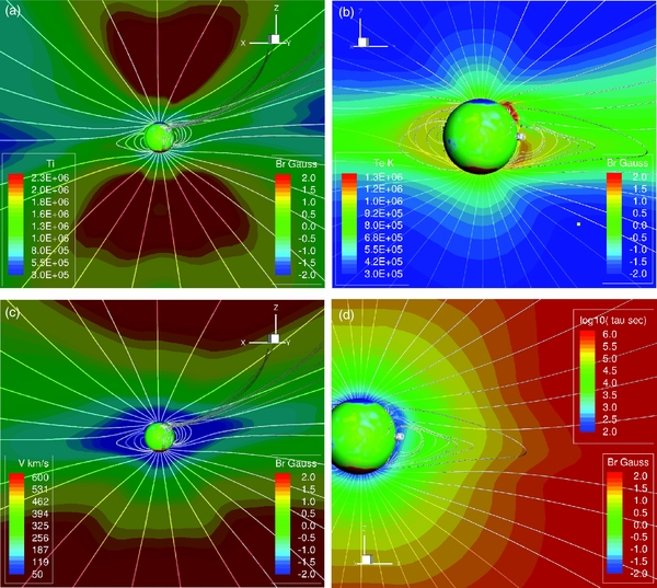
Figure 1. Initial state of the model corona. All panels show the magnetic field with white lines above a meridional slice of the of domain and the spherical inner boundary of the corona colored to show the radial magnetic field. Panels (a), (b), (c), and (d), respectively, show the ion temperature, electron temperature, solar wind velocity, and log (base 10) of the proton–electron Coulomb collision thermal relaxation time. Protons are heated over the poles on open field lines by the dissipation of Alfvén waves while electrons are heated by thermal conduction from the lower boundary.
Download figure:
Standard image High-resolution image2.3. CME Initiation
CME events originate from coronal magnetic fields that possess significant free energy, which are typically assumed to be of two forms: a magnetic flux rope (e.g., Low 1994; Gibson & Low 1998; Titov & Démoulin 1999; Chen & Krall 2003; Torok & Kliem 2005) or sheared magnetic arcades (e.g., Wu et al. 1991; Amari et al. 2003; Manchester 2003). For our simulations, we employ the flux rope model of Titov & Démoulin (1999, hereafter TD99), which was first used in a numerical simulation of CMEs by Roussev et al. (2003a) and in many following studies (e.g., Tóth et al. 2007; Lugaz et al. 2007; Manchester et al. 2008; Loesch et al. 2011; Evans et al. 2011). The CMEs in our model are initiated by linearly superimposing the semicircular flux rope upon the coronal field while line tying the flux rope to the inner boundary. The strapping field around the rope is not included so that the flux rope is in a state of force imbalance and is immediately expelled from the corona by the magnetic hoop force.
The primary concern of our study is the individual temperature structures of the protons and electrons. In particular, the temperature of the electrons will be dominated by rapid heat conduction along magnetic field lines. For this reason, we present two distinct simulations designed to explore the effects of field line geometry on electron heat propagation. In the first case, the flux rope is placed at the equator, embedded deep in the streamer belt (centered on the +y axis), and in the second case, the rope is placed in the high-latitude active region that produced the 2008 December 12 CME.
For the first simulation, the TD99 flux rope is defined by the following parameters: aspect ratio is 0.8; electric current is 2.5 × 10¹¹ A; the major radius is 6.0 × 10⁷ m; the minor radius is 9.0 × 10⁶ m. The center of the torus is submerged 1.25 × 10⁷ m below the boundary, and a mass of 5.0 × 10¹⁴ g is entrained in the flux rope to mimic the mass of a filament. For the second simulation, the flux rope differs in that the current is increased to 3.25 × 10¹¹ A and the mass is reduced to 1.0 × 10¹³ g. The purpose of the changes is to produce a faster CME more characteristic of an active region eruption.
These two configurations (streamer centered and active region) are shown, respectively, in panels (a) and (b) of Figure 2. The magnetic field lines are dawn in white, illustrating the flux rope by a highly twisted bundle of lines. In panel (b), the flux rope is oriented to match the observed magnetic polarities shown on the coronal boundary in color. The outer field lines of the rope connect directly to open field lines of the solar wind, which are colored purple. In contrast, the field lines of the rope shown in panel (a) are entirely connected to the inner boundary and have the same orientation as the field in the surrounding streamer to minimize reconnection.
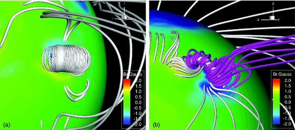
Figure 2. Panel (a) shows the structure of the coronal magnetic field with the flux rope inserted into a high-latitude active region. Here, the radial field strength at the coronal boundary is shown in color and field magnetic field lines are shown in white with the exception of those shown in purple, which show open field lines of the active region to which the flux rope is connected. Panel (b) shows the TD99 flux rope at the equator where its field roughly matches the surrounding field of the streamer belt.
Download figure:
Standard image High-resolution image3. RESULTS: THERMAL STRUCTURE OF THE CME-DRIVEN SHOCK
The CMEs initiated by the flux ropes rapidly accelerate to speeds faster than the ambient solar wind (800 km s−1 and 1000 km s−1 for the streamer and active region cases, respectively) and drive shocks that travel ahead of ejected plasma. In this model, both protons and electrons are accelerated and compressed equally at the shock, given the single velocity of the model. However, the thermodynamics for the particle species are entirely different as the shock is only supersonic relative to the proton fast-mode speed and not that of the electrons. As a result, the protons receive the kinetic energy dissipated at the shock, while the electrons are only heated by their adiabatic compression at the shock. The proton heating is very substantial as the fast-mode Mach number of the shock approaches a value of 5, similar to that of Manchester et al. (2005). There is also some heating of protons that occurs at the surface of the flux rope that results from numerical magnetic dissipation. In reality, this should be treated explicitly as Joule heating of electrons, which will be explored in future works. Here, we ignore this numerical heating and concentrate on the shock, which is properly treated.
The multi-component temperature structure of the CME can be seen 2 minutes after initiation in Figure 3. Panels (a) and (b) show an isosurface of the plasma speed at 800 km s−1 colored to show proton and electron temperature, respectively. Field lines of the erupting flux rope are colored white, expanding above the coronal boundary colored to show the radial field strength. The isosurface occurs in the sheath just behind the shock so that we see the full effect of shock heating. Proton temperatures are 45 MK near the nose of the shock and fall near 20 MK near the flanks of the shock. The electron temperature in contrast is more than an order of magnitude cooler and has the opposite radial variation, being coolest at the nose of the isosurface and hottest at the flanks. The contrast in proton and electron temperature is shown in more detail in panels (c) and (d) of Figure 3, which show, respectively, an isosurface of proton temperature (40 MK) colored to show electron temperature and an isosurface of electron temperature (3 MK) colored to show the proton temperature. We find that the shape of the temperature isosurfaces roughly corresponds to the velocity isosurface, with hotter protons found on the far side of the CME and hotter electrons found nearer to the Sun.

Figure 3. Three-dimensional views of the temperature structure of the CME seen from above the north pole 2 minutes after initiation. White lines illustrate the magnetic field comprising the flux rope. Panels (a) and (b) show an isosurface of plasma speed at 800 km s−1 colored to indicate proton and electron temperatures, respectively. Panels (c) and (d) show isosurfaces of proton and electron temperatures at 40 MK and 3 MK colored to show the temperatures of the electrons and protons, respectively. Protons are shock-heated to temperatures between 20 MK and 40 MK, while electrons are only briefly heated by collisions with protons to attain temperatures that are one tenth this magnitude.
Download figure:
Standard image High-resolution imageOn the velocity isosurface, the temperature gradient of the protons reflects the variation in Mach number of the shock, which is highest at the nose of the CME and along the axis of the expanding flux rope, and lowest in the polar directions orthogonal to the rope axis. Since the temperature jump at the shock is dependent on the Mach number squared, a small variation in the Mach number produces the factor-of-two variation in the temperature in the CME sheath seen in panels (a) and (d) of Figure 3. The CME heating of electrons is the result of Coulomb collisions with shock-heated protons. Given that the relaxation time is inversely proportional to the electron density, the stratification of the corona strongly affects the thermal relaxation time as shown in panel (d) of Figure 1. In the initial state, the thermal relaxation time is approximately 500 s at the top of the rope and 140 s at the base. It is this difference in relaxation time that produces the reversed radial temperature distributions of the electrons compared to the protons. After 2 minutes, the electrons at the base of the CME are hotter at 3.0 MK than those at the top at 2.4 MK even though the temperatures of the protons are at 27 MK and 45 MK, respectively. The energy exchange rate falls so rapidly that the particle populations never approach equilibrium. 120 s after initiation, the top of the flux rope has risen from 1.28 Rs to 1.51 Rs (with an average speed of 1340 km s−1) and the thermal relaxation time in the sheath furthest from the Sun has already increased to 4200 s. At this point, collisions are so infrequent that the particle populations thermodynamically decouple and the electrons never reach more than one tenth of the temperature of the protons in the CME sheath.
The continued evolution of the system is shown in Figures 4 and 5. Here, the temperature structure is illustrated at 8 and 16 minutes after CME initiation in the same format used in Figure 3, with one exception: panels (a) and (b) show the system in meridional perspective rather than equatorial. At these later times, the CME has slowed, so the velocity isosurfaces shown in panels (a) and (b) are at the value of 500 km s−1. Peak proton and electron temperatures have dropped to 20 MK and 2 MK, respectively. The shape of the 10 MK proton isosurfaces (panel (c)) is almost identical in size and shape to the velocity isosurface, clearly reflecting the shock heating of the protons. However, as a result of collisional decoupling and heat conduction, the electron isosurfaces become increasingly divergent from the protons. By 8 minutes, the shell of hot electrons that first formed in the CME sheath low in the corona now extends beyond the shock front. The electron isosurface at 2 MK (panel (d)) is found beyond the hot protons from the low corona to a cusp that extends beyond the velocity isosurface. At 16 minutes, the effects of heat conduction are very pronounced as seen by the shape of the electron temperature isosurface at 1.5 MK shown in panel (d). Here, the isosurface extends to 8.4 Rs on open field lines and to 4 Rs on closed field lines that form the tip of the helmet streamer. It is important to note that beyond the proton shock, these magnetic loops are not expanding outwards, but are still stationary.
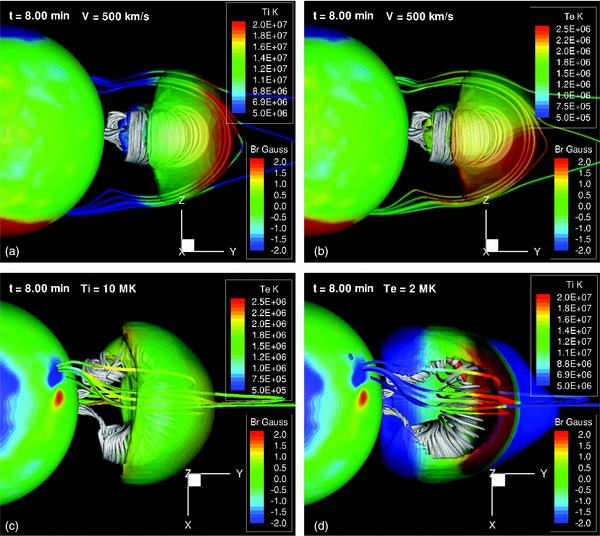
Figure 4. Three-dimensional views of the temperature structure of the CME 8 minutes after initiation. Panels (a) and (b) show a meridional view of an isosurface of plasma speed at 500 km s−1 colored to indicate proton and electron temperatures, respectively. Panels (c) and (d) show isosurfaces of proton and electrons temperature at 10 MK and 2 MK, respectively. These panels are viewed from the north pole showing the flux rope at the equator, with magnetic field lines shown in white. The isosurfaces are colored to show the temperature of the complementary species. Proton peak temperature has dropped to 20 MK, while heat conduction begins to extend hot electrons beyond the confines of the CME sheath.
Download figure:
Standard image High-resolution image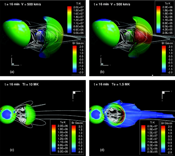
Figure 5. Three-dimensional views of the temperature structure of the CME 16 minutes after initiation. Panels (a) and (b) show a meridional view of an isosurface of plasma speed at 500 km s−1 colored to indicate proton and electron temperatures, respectively. Panels (c) and (d) show isosurfaces of proton and electrons temperature at 10 MK and 1.5 MK, respectively. These panels are viewed from the north pole showing the flux rope at the equator, with magnetic field lines shown white. The isosurfaces are colored to show the temperature of the complementary species. Proton peak temperature has dropped to 20 MK, while heat conduction extends hot electrons on open field lines far ahead of the CME.
Download figure:
Standard image High-resolution imageWhat is the conduit by which electrons on the open field lines and large loops are heated to 1.5 MK? By 16 minutes, the Coulomb thermal relaxation time in the sheath (where the field lines pass) has increased to 1.5 days, indicating that the hot electrons on these field lines could not come directly from collisions with protons behind the shock. However, close examination reveals that the closed field lines, which were populated with 3 MK electrons (at 2 minutes) extend very close to the footpoints of the large hot loops and open field lines. This proximity allows small amounts of numerical cross-field diffusion to heat the electrons on these more remote field lines. Heat conduction then allows the thermal energy to fill the closed streamer field lines and propagate far ahead of the CME on open field lines to form a precursor to the shock.
There are electron temperature asymmetries seen in panels (b) and (d) of Figure 4, where the electrons are cooler to the north side as compared to the south (1.8 MK compared to 2.3 MK). This difference reflects the temperature of the steady state corona surrounding the flux rope as seen in panel (b) of Figure 1. Here, we find a cool region (Te ≈ 0.8 MK) to the north of the flux rope and a hot region in the streamer belt on the south side of the rope (Te ≈ 1.2 MK). This roughly 0.4 MK temperature difference is maintained after the collisional heating of the electrons. The temperature asymmetry is found in the Te = 2 MK isosurface shown in panel (d) of Figure 4, where a hole is found on the north side of the surface and is closed to the south.
We next focus on the formation of a cavity of cool electrons that is seen in panels (d) of Figures 4 and 5. The early-phase coupling to shocked protons forms a nearly hemispherical shell of hot electrons, which extends down to the coronal boundary as a result of heat conduction. Inside this shell, the temperature of the electrons is close to the ambient level. Once the electrons decouple, they have no source of additional heating and they begin to cool by the adiabatic expansion. The result of this cooling forms the cavities seen in the electron temperature isosurfaces. By 16 minutes, the electrons in the cavity behind the toroidal rope have cooled to 0.8 MK (compared to 1 MK of the pre-event state) and are surrounded by a shell of hotter electrons at 1.6 MK in the plane of the toroidal rope.
Finally, we examine the temperature structure in the low corona shown in Figure 6 to find signatures of emission in the extreme ultraviolet. In Panels (a) and (b), we see the corona at times 8 and 16 minutes, respectively, shown with isosurfaces of electron temperature at 2 MK and 1.5 MK colored to show proton temperature. The electron temperature in the low corona is shown at a radius of 1.06 Rs, where we find an oval of elevated temperature that cools as it expands. The electron temperature of the oval is roughly at 1.8 MK at 8 minutes and falls to roughly 1.5 MK by 16 minutes. These temperatures are near the peaks in emission for both 193 Å and 195 Å bands, and 1.8 MK also falls very close to the peak for 211 Å. Thus, in the extreme ultraviolet, there would be an obvious manifestation of a bright ring expanding for the location of the CME, which is consistent with waves first observed in the extreme ultraviolet (Dere 1997; Thompson et al. 1998) with the Extreme-ultraviolet Imaging Telescope (EIT; Delaboudiniére et al. 1995) on board the Solar and Heliospheric Observatory (Domingo et al. 1995). Furthermore, at 8 minutes, we find heating near the base of the flux rope, which is the result of magnetic dissipation and a clear proxy for flare heating.

Figure 6. Three-dimensional views of the temperature structure of the CME. Panels (a) and (b) show isosurfaces 8 and 16 minutes after initiation at values of Te equal to 2 MK and 1.5 MK, respectively, both colored to show proton temperature. The spherical surface shows the temperature in the low corona at a height of r = 1.06 Rs. The oval of elevated temperature results from a CME-driven compressional wave passing through the low corona, which heats electrons to values of 1.8 MK and 1.5 MK, respectively. Panel (c) shows the proton temperature on the equatorial plane and on field lines passing through the wave (also colored to show proton temperature), while the flux rope is shown with white lines. Panel (d) shows line plots of the proton and electron temperatures along with velocity and proton sound speed as a function of x along the line passing through the compression wave that is shown in panel (c). These lines show the presence of a fast-mode wave propagating through the low corona that compresses the plasma, elevating the proton and electron temperatures.
Download figure:
Standard image High-resolution imageTo better understand the brightening, we give a close-up view of the proton temperature on the equatorial plane at 8 minutes as shown in panel (c) of Figure 6. Here, we find that the proton temperature is above 3 MK far behind the shock, and then falls below 2 MK at a height of 1.17 Rs, marking the transition from a fast-mode shock wave to a fast-mode wave in the low corona. Panel (d) shows line plots of proton and electron temperatures, plasma flow speed (ux), sound speed, and electron density as functions of horizontal distance, x, along the straight white line shown in panel (c), This line passes within a distance 1.1 Rs from the solar center, where the plots clearly show the elevation of both proton and electron temperatures associated with the compressive wave. An increase in the magnetic field strength at the wave front confirms that the wave is of the fast-mode MHD variety. With identical velocities, the protons and electrons receive the same compression, which increases the density 60% to a value of 1.6 × 109 cm−3. For protons, the process is nearly adiabatic, while electrons experience heat conduction that transports thermal energy ahead of the compression and reduces the peak temperature at the wavefront to 1.8 MK compared to 2 MK found for protons. Thus, even at this low height in the corona, it is clear that Coulomb collisions are unable to equilibrate the proton and electron temperatures on the timescale of a passing wave. Behind the wave, the proton temperatures rise to more than 3 MK as a result of magnetic dissipation near the footpoints of the flux rope.
Our model again provides an example of CME-driven fast-mode MHD waves as a mechanism capable of producing EIT waves as has been proposed by previous authors (e.g., Thompson et al. 1999; Klassen et al. 2000; Vrsnak et al. 2002; Cliver et al. 2004) and previously illustrated by way of numerical simulation (e.g., Wu et al. 2001; Ofman & Thompson 2002; Delannée et al. 2008; Cohen et al. 2009; Downs et al. 2011). In particular, our work resembles that of Cohen et al. (2009), employing the same numerical code and also the same flux rope initiation mechanism for the CME. Our model shows the increase in both density and temperature that would produce a significant brightening in the extreme ultraviolet in the 193, 195, and 211 Å bands. What we do not find are conditions for enhanced coronal emission in the low corona resulting from electron heat conduction. When heat propagates back from the CME-driven shock front to the low corona, it is effectively absorbed by the much denser lower atmosphere so that by the time the heat front reaches a height of 1.1 Rs, it has a negligible warming effect that is much smaller than the heating caused by the compressional wave.
3.1. Active Region CME
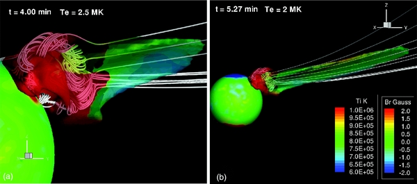
Here, we briefly describe the result of the second simulation in which the flux rope is placed in the high-latitude active region that produced the CME of 2008 December 12. The purpose here is not to produce the specific features of that event, but to investigate the properties of CME-related heat conduction in more complex circumstances. A feature of this active region is open magnetic flux to which the magnetic flux rope directly connects when inserted into the corona as shown in panel (b) of Figure 1. The temperature structure of the CME is shown in Figure 7. Here, panel (a) shows the CME 4 minutes after initiation with an isosurface of electron temperature at 2.5 MK colored to show proton temperature. The temperature scale is highly saturated to show the proton temperature far from the shock. Panel (b) shows the system at 5.27 minutes after initiation with an isosurface of electron temperature at 2 MK.
Figure 7. Three-dimensional views of the CME launched from an active region in the northern hemisphere. Panels (a) and (b) show isosurfaces of electron temperature at 2.5 MK and 2 MK, respectively, colored to show proton temperature. Peak proton temperatures are comparable to those found in the first simulation, but the color scale is chosen to show the low proton temperature far from the Sun. The coronal boundary is colored to show the radial field while white lines illustrate the magnetic field showing the eruption of a distorted flux rope, which is directly connected to open field lines in the solar wind. Energized by collisions with shock-heated protons, hot electrons immediately conduct their heat on these open lines away from the CME at speeds of the order of 104 km s−1.
Download figure:
Standard image High-resolution image
The salient feature of this model is the hot electron precursor that precedes the proton shock and travels more than 10 times faster than the CME. Like the previous model, the electrons are heated by collisions with shock-heated protons low in the corona. Unlike the previous model, the shock forms on open field lines where heat conduction can immediately transport the thermal energy away from Sun. An analysis of the speed of the heat propagating shows that at 3 MK, the front moves at approximately 104 km s−1, which compares favorably with the thermal speed of electrons at this temperature, which is 8.7 × 10³ km s−1. However, there is a tail to the heat front that extends out further at lower temperatures.
4. SUMMARY AND CONCLUSIONS
The simulations discussed here show the great richness and complexity of the thermal structure of CME-driven shocks that occur when electrons and protons are treated independently with electron heat conduction, proton shock heating, and Coulomb collisions coupling the two species. The protons show a pattern of shock heating found in simpler single-species models, namely a hot sheath region that reaches temperatures above 20 MK. The electrons are far different in their behavior. With thermal speeds far greater than protons, they do not directly experience CME-driven shocks but are carried along by electrostatic forces to maintain charge neutrality. Electrons briefly couple by collisions to protons (within 2 Rs), only long enough to reach one tenth of the proton temperature found in the sheath of a fast CME. This basic result was found by Kosovichev & Stepanova (1991) and Stepanova & Kosovichev (2000), who show similar unequal electron and proton temperatures behind coronal shocks. In addition, we show the results of field-aligned heat conduction in complex geometries. The thermal content of electrons conducts along magnetic field lines at a speed approximately equal to the thermal speed of the electrons (≈104 km s−1). In a system with a closed field line geometry, the heat remains trapped until the closed field lines reconnect with open field lines, or cross-field diffusion allows the heat to migrate on to open field lines allowing the heat to escape. In systems with open field lines extending low in the corona where the CME-driven shock forms, heat conducts ahead of the shock to immediately form a shock precursor in the form of hot electrons.
This simulation shows that there are significant dynamical and observational consequences of the thermodynamic decoupling of protons and electrons in the corona. The fact that this decoupling occurs so rapidly effectively cuts in half the ability of the plasma to absorb the energy dissipated at shocks. Consequently, at distances beyond 1.5 Rs, shock-heated protons will be twice as hot as predicted by a two-species, single-temperature model. This fact is seen in Figure 7 of Manchester et al. (2004), which shows the total temperature, which in the absence of electron heating at the shock correctly matches the proton temperature of 20 MK found in the sheath of the low-latitude CME at 8 minutes. The heating of protons and other ions to tens of MK has significant implications for the seed population of energetic particles necessary for diffusive shock acceleration. This acceleration mechanism requires that particles have sufficient initial energy upon the first collision to cross upstream of the shock. This population of energetic particles is assumed to come from the shocked ions, specifically from the high-energy tail of the Maxwellian or kappa distribution (e.g., Treumann 2009), which will naturally be increased with increased ion temperature.
The electron heat conduction also has significant implications for observations made in the extreme ultraviolet, the emission levels of which are highly sensitive to electron temperature. As shown in Figure 6, protons and electrons decouple on the timescale of the passage of the CME-driven compression wave, which allows heat conduction to significantly lower the temperature of the electrons from 2.0 to 1.8 MK. Similarly, on the timescale of impulsive flares, there will necessarily be significant departures from the proton and electron temperatures, which will strongly affect the flare emission in the extreme ultraviolet. Any model hoping to quantitatively reproduce EIT waves or flare emission must address electron–proton collisional coupling along with electron heat conduction.
As complex as this model may be, reality is far more complicated. We have assumed a priori that electrons and protons are thermodynamically coupled only by Coulomb collisions. In fact, there are other mechanisms that can couple these particle populations and more rapidly thermalize the electrons (e.g., Wu et al. 1984). Evidence of electron heating at collisionless shocks is presented by Schwartz et al. (1988), who analyzed 66 terrestrial bow shock and 14 interplanetary shock crossings. They found on average electrons receive 20% of the total temperature jump at shocks. The electron heating (as a fraction of total heating) is inversely proportional to Mach number. At low Mach numbers, 50% of the heat may go to electrons and at high Mach numbers this value drops to less than 10%. The heating of electrons is purely transverse to the magnetic field with perpendicular temperature increasing in direct proportion to the magnetic field strength increase across the shock. Ghavamian et al. (2001) found additional evidence of electron heating when they modeled the spectroscopic properties of supernova remnants formed by high Mach number collisionless shocks. They too find an inverse correlation between magnetosonic Mach number and electron thermal equilibration, which is consistent with Schwartz et al. (1988). Our results then should be considered as a limiting case of minimum thermal coupling between electrons and protons, which is most appropriate for strong or parallel shocks.
Far from the Sun, in the absence of collisions, the particles become free-streaming. However, the electrons can not escape the Sun at their thermal speed because the interplanetary electric potential (Jockers 1970) limits charge separation and results in a net zero electric current from the Sun. Electron heat flux must ultimately depart the Sun at the bulk flow speed of protons. Furthermore as electrons propagate from the Sun, they will undergo magnetic focusing as the interplanetary magnetic field decreases in strength. On closed field lines, the hot electrons we find in our model will form oppositely directed beams that may contribute to the suprathermal electrons found in ICMEs (Gosling et al. 1987). Far from the Sun, electrons will continue to be heated at the CME-driven shock by adiabatic compression and possibly energized by additional mechanisms. These energized electrons have been found to leak out from compression regions and produce field-aligned electron beams directed away from the shock as noted by Steinberg et al. (2005).
In order to treat these phenomena, there are several limitations of the model that should be addressed in future work. First, our simulations can only address the isotropic core population of electrons and neglects the strahl and suprathermal halo populations, which require nontheramal sources that often produce temperature anisotropies. For example, Vocks et al. (2008) show that the quiet solar corona is capable of producing suprathermal electrons by resonant interaction between electrons and Whistler waves. Second, heat conduction is treated with a diffusion formulation, which allows heat transport at speeds faster than the thermal speed of the electrons. Flux-limited diffusion (see, for example, van der Holst et al. 2011) needs to be applied to prevent this excessively fast transport. Third, Spitzer conductivity is valid only in a collision-dominated plasma. To extend our simulations to 1 AU, we need to formulate a natural transition to collisionless heat conduction that addresses the free-streaming of particles. Fourth, the conservative formulation of the code converts all dissipated energy to proton thermal energy. This ensures jump conditions at shocks but is inappropriate for magnetic dissipation. In the latter case, the energy should go preferentially to the electron population. We need to explicitly treat Ohmic dissipation and ensure that the explicit terms always dominate the numerical dissipation at the locations of strong magnetic gradients. For the purpose of this paper, we have restricted our attention to shock heating, which is much more significant than Joule heating near strong shocks.
W. Manchester was supported by NASA grants LWS NNX09AJ78G and NNX11AN38G, and B. van der Holst was supported by grant LWS NNX09AJ78G. We gratefully acknowledge the supercomputing resources with which these simulations were performed: the Pleiades system provided by NASA's High-End Computing Program under award SMD-11-2364.