


ABSTRACT
The recently protracted solar minimum provided years of interplanetary data that were largely absent in any association with observed large-scale transient behavior on the Sun. With large-scale shear at 1 AU generally isolated to corotating interaction regions, it is reasonable to ask whether the solar wind is significantly turbulent at this time. We perform a series of third-moment analyses using data from the Advanced Composition Explorer. We show that the solar wind at 1 AU is just as turbulent as at any other time in the solar cycle. Specifically, the turbulent cascade of energy scales in the same manner proportional to the product of wind speed and temperature. Energy cascade rates during solar minimum average a factor of 2–4 higher than during solar maximum, but we contend that this is likely the result of having a different admixture of high-latitude sources.
Export citation and abstract BibTeX RIS
1. INTRODUCTION
The recently protracted solar minimum offers an excellent opportunity to study both the intensity and anisotropy of the turbulent cascade within the solar wind at a time of very low solar activity. It was once widely held that fluctuations in the solar wind were remnant Alfvén waves originating within the near-corona acceleration region of the solar wind (Coleman 1966; Barnes 1979). Later, it became evident that the fluctuations constitute a magnetodynamic analog to traditional hydrodynamic turbulence (Coleman 1968; Matthaeus & Goldstein 1982). While there is clear evidence of in situ evolution of the turbulence (Matthaeus & Velli 2011), it is more difficult to assess the role of possible sources. In particular, one can ask whether the fluctuations at 1 AU are primarily the result of in situ generation or are they mainly solar in origin? Admittedly, this is a somewhat artificial distinction since all solar wind energy originates with the Sun. Our question is whether persistent regions of strong shear act to inject energy into the inertial range, as might be the case during solar maximum. The alternative is that long-lived large-scale fluctuations that pervade the flow act to drive the inertial range turbulence in a more homogeneous manner or the general absence of shear allows the fluctuations to be long-lived wave modes.
Shear drives turbulence. Single-spacecraft analyses provide no clear and unambiguous resolution of shear. It is the assumption of time-independent sources and radially independent wind speed that permits us to estimate wind shear and these assumptions are limited. Therefore, during solar minimum when the flow is characterized by corotating interaction regions (CIRs) separated by slowly varying wind speeds it is easy to imagine that the only significant wind shear resides within the CIR while the surrounding flow is essentially shearless.
Within this context, the turbulence observed during solar minimum may be considered a likely remnant of solar activity as the only strong shears observed are the CIRs that are typically far apart and unable to generate significant turbulent activity in the space between them (Borovsky & Denton 2010; Smith et al. 2011; Tessein et al. 2011). There is even a larger question that stems from the observation during solar minimum of long-duration intervals that persist far from regions of strong shear. With a quiet Sun and little local shear, we can ask, "Are these regions turbulent at all?" or are they better described by non-interacting wave theory as was once thought? The cross-correlation between magnetic and velocity fluctuations can be large in the fast wind regions which may be consistent with weakly turbulent conditions. Therefore, the fluctuations seen at this time might be expected to have different properties than what is seen during more active phases of the solar cycle when large-scale shears and solar activity are more plentiful at low latitudes.
We can address the most basic of these questions, "How does the turbulent energy cascade compare during solar minimum versus solar maximum?" by employing third-moment techniques (Politano & Pouquet 1998a, 1998b; MacBride et al. 2005, 2008; Podesta et al. 2007; Podesta 2008; Stawarz et al. 2009, 2010, 2011; Sorriso-Valvo et al. 2007, 2010; Marino et al. 2008; Carbone et al. 2009; Smith et al. 2009, 2010; Wan et al. 2009, 2010a, 2010b; Forman et al. 2010; Osman et al. 2011). These methods originated in hydrodynamics (Kolmogorov 1941; Yaglom 1949) and the theory was extended to include incompressible magnetohydrodynamics (MHD) by Politano & Pouquet (1998a, 1998b). MacBride et al. (2005, 2008) developed the formalism for application to the solar wind using single-spacecraft techniques that were subsequently applied and refined by other authors. Wan et al. (2009, 2010a) raised the issue of large-scale shear and modified the formalism. Both Wan et al. (2010b), who performed numerical studies, and Stawarz et al. (2011), who studied solar wind observations, concluded that these additions are not necessary when studying a balanced admixture of positive and negative shear regions. The key feature of the formalism is this: all that is assumed in the derivations is incompressibility, homogeneity, geometry, and scale separation while homogeneity can be suspended to address regions of persistent large-scale shear. Scale separation means that the inertial range is energy conserving while the smaller scales are energy dissipative. Otherwise, there are no assumptions regarding specific dynamics or approximations to the dynamical equations. We will assume a stationary turbulent spectrum that predicts a linear scaling of third-moment expressions.
Stawarz et al. (2009) applied the formalism to years surrounding solar maximum using data from the Advanced Composition Explorer (ACE) spacecraft (McComas et al. 1998; Smith et al. 1998; Stone et al. 1998). They found that the energy cascade rates, regardless of what geometry was assumed for the purpose of completing the analysis, were in good agreement with the average measured rate of proton heating at 1 AU. MacBride et al. (2008) demonstrated that the perpendicular cascade of energy across the mean magnetic field was greater than the parallel cascade when measured within fast winds. This was argued to be a direct measurement of the dynamic that attempts to create two-dimensional (2D) turbulence when a mean magnetic field is present (Shebalin et al. 1983) and the turbulence is not yet in that state (Dasso et al. 2005).
Section 2 reviews derivations of third-moment theory as applied to MHD and the solar wind. In Section 3, we apply these expressions to solar wind observations by the ACE spacecraft at 1 AU while distinguishing solar maximum years 1998–2004 from solar minimum years 2007 to 2009. Section 4 discusses the implications of this analysis. Lastly, we summarize our results.
2. THEORY
We follow the same data analysis procedures as described in Stawarz et al. (2009). The expression describing the inertial range energy cascade and assuming an isotropic geometry can be written as
where τ is the positive time lag and ∑i is the sum over all components. The cascade rate of (Z±)2 is given by  ±. The Elsässer variables are defined as

where V and B are the velocity and magnetic field measurements, respectively, and ρ is the mass density. The subscript "R" denotes the Radial component directed from the Sun's center to the point of measurement. The total energy cascade is given by T = (+ + −)/2. Because the outward propagating fluctuations tend to be energetically dominant at 1 AU, we prefer to accumulate the variables
A second possible geometry is derived from assuming that only the parallel and perpendicular wave vectors are energized. This is the hybrid geometry. To apply this concept, we rotate the data to mean field coordinates (Belcher & Davis 1971; Bieber et al. 1996):


where  is the unit vector in the radial direction and
  is the unit vector in the direction of the mean interplanetary magnetic field. The
  direction is the only perpendicular direction for which we have a measured nonzero lag because
  is perpendicular to the wind velocity and gives no measured lag. In principle, any lag across the mean field direction could be used to measure the perpendicular cascade, but in this coordinate system only the
  direction provides a finite lag perpendicular to the mean magnetic field. The resulting form for the perpendicular cascade is
while the parallel cascade is given by
The ∥ and ⊥ forms of the hybrid MHD cascade expression are independent and can be obtained simultaneously from the data (MacBride et al. 2008). The total energy cascade in the hybrid formalism is then given by TH = (out∥ + out⊥ + in∥ + in⊥)/2. Likewise, we can measure the anisotropy of the cascade by computing ⊥/∥ ≡ (out⊥ + in⊥)/(out∥ + in∥). We can sum ∥ and ⊥ cascades to get the cascade associated with outward and inward propagation
where L⊥ = VSWτsin ΘBR, L∥ = VSWτcos ΘBR. From the axisymmetric form we can recover the isotropic cascade if out/in∥ = (1/2)⊥out/in as there are two dimensions to the ⊥ cascade. We interpolate individual estimates of the third moments onto a common spatial grid L that is defined by taking 64 s data in a 450 km s−1 wind.
3. ANALYSIS
Application of these expressions to solar wind data is straightforward. We employ 64 s merged MAG and SWEPAM data from the ACE spacecraft. For the purposes here we will define the solar minimum years to be 2007–2009. The analysis is based upon 12 hr intervals from which the mean field is computed. We remove shocks and their upstream regions and driver gases by excluding data from 12 hr before the shock to 36 hr after the shock. Results are accumulated on a grid of common spatial lag through interpolation of the measured functions D3, which are averaged once the data are fully processed, and errors are propagated according to Gaussian statistics (Smith et al. 2010).
Vasquez et al. (2007) studied published analyses of Helios observations listing average radial gradients of proton temperatures in combination with ACE observations to derive an expression for the proton heating rate per unit mass at 1 AU:

where VSW is the solar wind speed in km s−1 and TP is the proton temperature in units of Kelvin. This expression is based on an r−0.9 radial dependence of TP. We will use this as our "ground truth" analysis.
Figures 1 and 2 show the computed average third-moment functions for the isotropic and hybrid analyses. Many of these functions show diverging results for lags greater than ∼2000 s with greater uncertainties and less linear trending at the longer lags. At longer lags, there is a noticeable and generally systematic difference between the D3 associated with outward and inward propagation that is absent at the shorter lags. This is separate from the parallel and perpendicular differences.
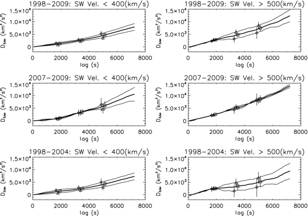
Figure 1. Analysis of measured third-order structure functions D3. Left: slow wind VSW < 400 km s−1 and (right) fast wind >500 km s−1. Top panels: ACE data years 1998–2009, (middle panels) solar minimum years (2007–2009), and (bottom panels) solar maximum years (1998–2004). Flux associated with Zout (diamonds) and Zin (triangles) with D3 function for total energy transport (squares with thicker lines). Note that in slow wind both Zout and Zin cascade at comparable rates while in the fast wind there tends to be a greater separation with the energy associated with outward propagation (generally the dominant energy term) cascading more rapidly than inward propagation.
Download figure:
Standard image High-resolution image
Figure 2. Same as Figure 1 except using hybrid geometry analysis. Solid curves are 2D component and dashed curves are 1D field-aligned component.
Download figure:
Standard image High-resolution imageMatthaeus et al. (2005) performed a multi-spacecraft analysis of the autocorrelation length at 1 AU and concluded that on average the autocorrelation length was shorter than previously thought. They obtained values of ∼1.2 M km or ∼44 minutes at an average wind speed of 450 km s−1. This suggests that the disagreement we observe at longer lags in both analyses may result from the energy-containing range rather than the inertial range, and so we decided here to average estimates for the energy cascade rate using only lags up to 1920 s which equals 30 lag steps of 64 s on the interpolated grid. Averages over longer lags yield comparable results, but tend to show slightly less agreement with the Vasquez et al. (2007) results and greater uncertainties. Moreover, use of longer lags may be theoretically incorrect if they extend outside the inertial range.
Figure 1 shows the computed values for D3, ISO where the data are subsetted both for time and average wind speed. The subset for time (top down) shows D3, ISO for the total ACE data set (1998–2009), solar minimum years (2007–2009), and the broadly defined solar maximum years (1998–2004). The latter is a subset of the interval studied by Stawarz et al. (2009) and selected to better represent solar maximum. The most immediate aspects of the figure are that the forms for D3 are essentially linear with lag as expected for lags up to 1920 s. The slope of each line yields the energy cascade rate associated with that interval of time and wind speed.
Table 1 lists the computed cascade rates associated with Figure 1. Note that the fast wind cascade consistently exceeds the slow wind cascade during both solar maximum and solar minimum, suggesting a greater in situ heating rate for fast winds. This is generally consistent with the Vasquez et al. (2007) result.
Table 1. Energy Cascade Rates for Figure 1
| Slow Wind | Fast Wind | |||||
|---|---|---|---|---|---|---|
| Years | out |
in |
T |
out |
in |
T |
| (× 103 J kg−1 s−1) | ||||||
| 1998–2009 | 1.31 ± 0.08 | 0.68 ± 0.05 | 1.00 ± 0.05 | 1.68 ± 0.14 | 2.35 ± 0.11 | 2.01 ± 0.09 |
| 2007–2009 | 0.50 ± 0.15 | 0.97 ± 0.12 | 0.71 ± 0.09 | 1.58 ± 0.19 | 2.24 ± 0.11 | 1.91 ± 0.11 |
| 1998–2004 | 1.70 ± 0.12 | 0.50 ± 0.08 | 1.10 ± 0.07 | 1.37 ± 0.23 | 2.03 ± 0.18 | 1.70 ± 0.15 |
Download table as: ASCIITypeset image
Table 2 lists both the number of 12 hr samples used to compute each of the curves in Figure 1 along with the average normalized cross helicity σc ≡ 〈δV · δB〉/〈ET〉, where δV and δB are the velocity and magnetic fluctuations, respectively, and ET is the total energy. As anticipated, the fast wind samples have, on average, greater normalized cross helicity than the slow wind samples consistent with the view that fast winds are dominated by outward propagating fluctuations. However, the fast wind samples also show greater cascade levels, on average, than the slow wind samples, suggesting that this level of cross helicity is insufficient to significantly alter the total energy cascade rate. Smith et al. (2010) and Stawarz et al. (2010) examined this question and did find evidence of reduced cascade rates at times of high |σc|, but the degree of dependence varied with the turbulent energy level.
Table 2. Statistics for Figures 1 and 2
| Slow Wind | Fast Wind | |||
|---|---|---|---|---|
| Years | No. of Samples | 〈σc〉 | No. of Samples | 〈σc〉 |
| 1998–2009 | 1581 | 0.463 ± 0.003 | 1651 | 0.743 ± 0.002 |
| 2007–2009 | 277 | 0.346 ± 0.007 | 486 | 0.681 ± 0.003 |
| 1998–2004 | 1158 | 0.502 ± 0.003 | 1032 | 0.779 ± 0.002 |
Download table as: ASCIITypeset image
Figure 2 shows the results of the hyrbid analysis and the computed D3, ⊥ (solid curves) and D3, ∥ (dashed curves) for the same data subsets shown in Figure 1. Table 3 gives the computed ∥ and ⊥ energy cascade rates for fast and slow winds during each of the three time intervals. Limiting our analysis to the first 1920 s of each fast wind panel in Figure 2, we note that the ⊥ cascade is consistently greater than the ∥ cascade throughout the solar cycle. This is not true of the slow wind intervals where the two components show statistically equivalent cascade rates at solar maximum, but statistically zero ⊥ cascade at solar minimum. We do not understand the slow wind result at solar minimum as it seems to lie outside the conventional theory for MHD cascade. This systematic anisotropy of the third moments for fast and slow winds was first observed by MacBride et al. (2008) who argued that this documented the evolution of the fast wind geometry away from field aligned wave vectors (Dasso et al. 2005) that dominate the large-scale fluctuations and toward the expected 2D state. While the slow wind is already dominated by a 2D geometry at the large scales, we cannot argue why a similarly anisotropic cascade is not seen that would transform the slow wind geometry into a more significantly 2D state.
Table 3. Energy Cascade Rates for Figure 2
| Years | ∥ |
⊥ |
TH |
⊥/∥ |
|---|---|---|---|---|
| (× 103 J kg−1 s−1) | ||||
| Slow Wind | ||||
| 1998–2009 | 0.55 ± 0.08 | 0.48 ± 0.06 | 0.99 ± 0.10 | 0.87 ± 0.16 |
| 2007–2009 | 0.48 ± 0.16 | −0.05 ± 0.11 | 0.53 ± 0.22 | −0.11 ± 0.24 |
| 1998–2004 | 0.58 ± 0.11 | 0.59 ± 0.08 | 1.07 ± 0.14 | 1.01 ± 0.24 |
| Fast Wind | ||||
| 1998–2009 | −0.25 ± 0.07 | 2.66 ± 0.10 | 2.37 ± 0.12 | −10.5 ± 2.96 |
| 2007–2009 | 0.51 ± 0.07 | 2.42 ± 0.16 | 2.93 ± 0.17 | 4.77 ± 0.76 |
| 1998–2004 | −0.41 ± 0.11 | 2.26 ± 0.16 | 1.71 ± 0.19 | −5.54 ± 1.54 |
Download table as: ASCIITypeset image
Figure 3 (bottom) plots the total energy cascade rates derived from D3 using both the isotropic and hybrid geometries as a function of the product VSWTP for the years 2007–2009. See Table 4 for tabulated cascade rates. Seven overlapping bins of VSWTP are used in accord with Figures 2 and 3 of Stawarz et al. (2009). As with the Stawarz et al. (2009) analysis, there is good agreement between the Vasquez et al. (2007) prediction for the proton heating rate and the computed energy cascade rates for both geometries. This means that for average parcels of solar wind plasma with a given product VSWTP, the turbulent cascade rate is the same regardless of the phase of the solar cycle. In this sense, the turbulence level during solar minimum is the same as for solar maximum. The total energy cascade according to the hybrid analysis can be as much as 30% greater than the cascade in the isotropic geometry, but both are in general agreement with the Vasquez et al. (2007) analysis and appear to be generally similar to the solar maximum analysis of Stawarz et al. (2009). We do note the systematic difference between computed proton heating rates and energy cascade rates derived from third-moment analyses whereby the computed cascade rates tend to be less than the heating rates for slow, cold winds and greater than the heating rates for fast, hot winds (Stawarz et al. 2009).

Figure 3. Top: ratio of cascade rate perpendicular to the mean field to the cascade rate parallel to the mean field: ⊥/∥. Bottom: analysis of solar minimum years (2007–2009) broken down into seven bins of VSWTp according to the Vasquez et al. (2007) analysis of local heating rates. Plot shows the computed total energy cascade rates using only the first 30 lags = 1920 s. Traditional Navier–Stokes formalism for isotropic geometry (squares) and MHD formalism for isotropic (diamonds) and hybrid geometries (triangles) are shown. Vasquez et al. (2007) analysis represented by "+" symbols.
Download figure:
Standard image High-resolution imageTable 4. Energy Cascade Rates for Figure 3
| VSWTP | Isotropic | Hybrid | Hydro |
|---|---|---|---|
| (× 106 K km s−1) | (× 103 J kg−1 s−1) | ||
| 2–20 | 0.08 ± 0.04 | 0.64 ± 0.11 | 0.10 ± 0.01 |
| 11–30 | 0.33 ± 0.05 | 0.70 ± 0.11 | 0.15 ± 0.02 |
| 20–40 | 1.07 ± 0.08 | 1.31 ± 0.16 | 0.33 ± 0.04 |
| 30–80 | 2.59 ± 0.10 | 4.88 ± 0.33 | 0.92 ± 0.05 |
| 40–120 | 3.16 ± 0.11 | 5.39 ± 0.30 | 1.43 ± 0.06 |
| 80–260 | 4.86 ± 0.17 | 6.19 ± 0.21 | 3.20 ± 0.12 |
| 120–400 | 6.86 ± 0.36 | 8.78 ± 0.49 | 5.22 ± 0.24 |
Download table as: ASCIITypeset image
Figure 3 (top) plots the computed anisotropy for the turbulent cascade using the hybrid analysis. See Table 5 for tabulated values of the cascade anisotropy. The bin with highest VSWTP value is omitted from the plot as the uncertainty is larger than the range of values plotted. The number is essentially meaningless. An isotropic cascade is represented by ⊥/∥ = 2 since there are two perpendicular directions. The anisotropy favors the field-aligned direction in four out of six bins and is isotropic in another. Only one bin shows a distinct preference for a 2D cascade. This may be a manifestation of the approximations used in our hybrid analysis or possibly the result of solar wind expansion leading to additional preferred directions of cascade.
Table 5. Energy Cascade Rate Anisotropies for Figure 3
| VSWTP | ∥ |
⊥ |
⊥/∥ |
|---|---|---|---|
| (× 106 K km s−1) | (× 103 J kg−1 s−1) | ||
| 2–20 | 0.48 ± 0.09 | 0.14 ± 0.06 | 0.30 ± 0.13 |
| 11–30 | 0.32 ± 0.10 | 0.33 ± 0.06 | 1.05 ± 0.37 |
| 20–40 | 0.49 ± 0.14 | 0.79 ± 0.07 | 1.61 ± 0.50 |
| 30–80 | 3.40 ± 0.31 | 1.48 ± 0.10 | 0.44 ± 0.05 |
| 40–120 | 3.30 ± 0.28 | 2.11 ± 0.12 | 0.64 ± 0.06 |
| 80–260 | 1.54 ± 0.09 | 4.65 ± 0.18 | 3.01 ± 0.22 |
| 120–400 | 0.12 ± 0.26 | 8.74 ± 0.41 | 71.1 ± 148 |
Download table as: ASCIITypeset image
Figure 4 shows the computed energy cascade rates as a function of year from 1998 through 2009. Table 6 lists average wind speeds and temperatures for each year showing that the rise in proton heating rates during solar minimum is due to increases in both the average wind speed and temperature. Surprisingly, solar minimum proves to be a time of elevated cascade rates and elevated heating rates at 1 AU relative to solar maximum conditions. Any suggestion that solar minimum is a time of greatly reduced interplanetary turbulence is not supported by this analysis. At the same time we must acknowledge that the yearly variation is a factor of 2–4 times the average, so one might claim that interplanetary turbulence is surprisingly constant in intensity throughout the changing solar cycle.

Figure 4. Top: plot of monthly sunspot number as a function of time. Bottom: analysis of average energy cascade rates as a function of year throughout the ACE mission. Analysis again limited to first 30 lags. Note that the average cascade rate increases during the protracted solar minimum. The interplanetary turbulence is far from dormant during these years of a relatively quiet Sun. Squares, diamonds, triangles, and "+" are defined as before.
Download figure:
Standard image High-resolution image
Table 6. Average Solar Wind Parameters for Figure 4
| Year | 〈VSW〉 | 〈TP〉 | 〈VSWTP〉 |
|---|---|---|---|
| (km s−1) | (× 104 K) | (× 107 km s−1 K) | |
| 1998 | 411.51 | 8.4 | 3.8 |
| 1999 | 439.58 | 9.5 | 4.6 |
| 2000 | 449.28 | 9.0 | 4.4 |
| 2001 | 422.06 | 8.5 | 3.9 |
| 2002 | 455.07 | 10.9 | 5.3 |
| 2003 | 548.77 | 15.1 | 9.1 |
| 2004 | 464.36 | 10.7 | 5.4 |
| 2005 | 472.04 | 10.4 | 5.5 |
| 2006 | 457.88 | 9.7 | 4.8 |
| 2007 | 499.89 | 11.1 | 6.0 |
| 2008 | 504.49 | 11.5 | 6.3 |
| 2009 | 418.74 | 7.0 | 3.1 |
Download table as: ASCIITypeset image
4. DISCUSSION
It is clear from this analysis that the turbulent cascade at 1 AU during the solar minimum years is as active as at any other time in the solar cycle. The average energy cascade rate exceeds the average computed for solar maximum years to a statistically significant degree. What we cannot tell from this analysis is whether the processes that convert the energy cascade into proton heat are in any way different at different times of the solar cycle or in different types of wind.
We have taken Vasquez et al. (2007) as the bench mark for solar wind proton heating rates. Analyses shown here raise questions about possible refinements in that analysis. For instance, Figure 3 shows that the computed third-moment cascade rates for both isotropic and hybrid MHD geometries exceed the solar wind proton heating rate when VSWTP is large, but is less than the computed proton heating rate when VSWTP is small. We do not know if this reflects the theory of Vasquez et al. (2007) or the limitations of the third-moment analysis (for instance, compressive shock heating is outside this theory and may contribute unequally to slow and fast winds).
Figure 4, in combination with Table 6, suggests that the yearly variation seen in heating and cascade rates may be in large part a sampling effect. First, both the average VSW and the average TP is elevated in 2007 and 2008. This suggests possibly different admixtures of solar sources including high-latitude winds. Zhao et al. (2009) use solar wind composition data and confirm that the solar wind at 1 AU consists of a larger percentage of coronal hole sources than during solar maximum. Second, the computed cascade rate exceeds the predicted heating rate during solar minimum while the cascade rates underestimate the heating rate during solar maximum. Figure 3 shows that our analysis of the cascade rate exceeds the expected heating rate at times of higher VSWTP. Therefore, the fact that our observations in Figure 4 show cascade rates greater than expected heating rates during solar minimum and less than expected heating rates at solar maximum is potentially a sampling imbalance between slow, cold wind and fast, hot wind that reflects the systematic trend seen in Figure 3. Solar maximum years contain a greater proportion of low-VSW, low-TP intervals leading to computed cascade rates that are less than heating rates and the reverse during solar minimum.
5. SUMMARY
We have realized in this analysis that there is a reproducible signature at 1920 s lags that may be associated with the autocorrelation scale (Matthaeus et al. 2005). For this reason and the need to limit our cascade analysis to inertial scales, we have limited our averages to lags less than this scale.
We have concentrated our analysis on determining the turbulent energy cascade at 1 AU during the solar minimum years and compared those results with time when the Sun is more active. We have again found that the anisotropic cascade of the fast wind is dominated by the perpendicular cascade which would seem to evolve the dominant field-aligned geometry (Dasso et al. 2005) toward a more 2D state. For reasons unknown, the slow wind cascade tends to be more isotropic.
Our analysis of the turbulent cascade at 1 AU indicates that the energy cascade during solar minimum is comparable to or exceeds the average cascade during solar maximum. Our application of the Vasquez et al. (2007) analysis also indicates a stronger thermal proton heating rate at this same time. The solar source is significantly quieter at solar minimum in terms of gross features such as sunspots and eruptions, and so the greater turbulence level may be initially unexpected. The solar wind at 1 AU contains a greater percentage of high-latitude sources during minimum and it is possible that the greater turbulence level associated with solar minimum is a selection effect of sampling in the ecliptic at a time when high-latitude sources become more visible. However, we have seen that the slow wind possesses an approximately equal cascade rate during solar minimum as it does during solar maximum and it is within a factor of three of the cascade rate for the fast wind.
In hindsight, it may be argued that we should have expected solar minimum to be a time of roughly equal turbulent cascade as turbulent transport models that make use of the time varying solar wind parameters such as Smith et al. (2006) and Oughton et al. (2011) fail to reveal strong solar cycle effects. Nevertheless, direct measurement of the energy cascade as the third-moment analysis permits is extremely revealing and speaks directly to the level of activity exhibited by the turbulence. In summary, the variation in slow and fast wind cascade rates for solar minimum and solar maximum is no more than a factor of 2–4 at most with surprisingly constant cascade and heating rates over all phases of the solar cycle.
The authors thank the ACE/SWEPAM team for providing the thermal proton data used in this study. J.T.C. and C.W.S. are supported by the Caltech subcontract 44A-1062037 to the University of New Hampshire in support of the ACE/MAG instrument. C.W.S. and M.A.F. are supported by the NASA Sun-Earth Connection Guest Investigator grant NNX08AJ19G. B.J.V. is supported by the NASA Guest Investigator grant NNX09AG28G, the NASA/SR&T grant NNX10AC18G, and the NSF/SHINE grant ATM0850705. J.T.C. is an undergraduate physics major at the University of New Hampshire. J.E.S. is now a graduate student at the University of Colorado at Boulder.