A GLOBAL TWO-TEMPERATURE CORONA AND INNER HELIOSPHERE MODEL: A COMPREHENSIVE VALIDATION STUDY

As the source of coronal mass ejections (CMEs) as well as solar wind, understanding the solar corona (SC) is critical for space weather forecasts. Although the physical origin of the hot corona and the expanding solar wind is still in debate, Alfvén wave acceleration of solar wind has been considered as one of the possible mechanisms (Belcher 1971; Jacques 1977). In this type of model, the wave pressure will accelerate the solar wind while the gradual dissipation of the waves can heat the plasma (Hollweg 1986). In the past two decades, a number of coronal models have been created that use Alfvén waves, e.g., Suzuki (2006) constructed a one-dimensional (1D) model that forecasts the solar wind speed at 1 AU, while, e.g., Lou (1994), Ofman & Davila (1995), Bravo & Stewart (1997), Ruderman et al. (1998), and Usmanov et al. (2000) analyzed the Alfvén waves in two-dimensional (2D). Usmanov et al. (2000) for the first time developed 2D global axisymmetric solar wind models with Alfvén waves. Fully three-dimensional (3D) solar wind models with Alfvén waves have been studied by, e.g., Evans et al. (2009) for the surface Alfvén wave damping mechanism, and van der Holst et al. (2010) developed a 3D solar wind model from the Sun to 1 AU that utilizes observational data for the boundary conditions. Sokolov et al. (2009) coupled the frequency-resolved transport equations for the Alfvén waves to the magnetohydrodynamics (MHD) equations for an arbitrary 3D domain. Partial reflection of Alfvén waves has also been investigated (e.g., Chandran & Hollweg 2009; Cranmer 2010; Verdini et al. 2010). Note that there are other mechanisms that could be responsible for coronal heating. One is reconnection between open and closed field lines. Reconnection is considered the most likely channel to convert magnetic energy to heat (e.g., Priest & Forbes 2000). Since only a small fraction of the coronal magnetic field is open to the heliosphere, the dominant source of energy should come from the stochastic reconnections between open and closed field lines (e.g., Fisk et al. 1999; Schwadron et al. 2006). Reconnection heating is more difficult for numerical modeling than wave heating mechanisms due to the multi-scale nature of magnetic reconnection. To accurately model the interaction between closed and open field lines, a fully 3D coronal magnetic field is needed. Some initial work with the reconnection heating mechanism can be found in Fisk (2005) and Tu et al. (2005). Parker (1983, 1988) also proposed a nanoflare coronal heating model, and there are many discussions and works since then (e.g., Cargill 1994; Klimchuk 2006; Aschwanden 2008; Janse & Low 2009). In nanoflare heating models, ohmic dissipation of electric currents is responsible for the coronal heating, which would preferentially heat electrons.

Another property that is important in the modeling of the SC as well as of the inner heliosphere (IH) is the different temperatures of electrons and protons. This occurs beyond ∼2 R_☉ where the collisions between these two species are infrequent (Hartle & Sturrock 1968). Different temperatures between electrons and ions have been found by the Solar and Heliospheric Observatory (SOHO)/Solar Ultraviolet Measurement of Emitted Radiation and SOHO/Ultraviolet Coronagraph Spectrometer (Seely et al. 1997; Tu et al. 1998). A more thorough investigation of different temperatures between electrons and ions is made by Landi (2008) and Landi & Cranmer (2009). The model effects have been extended to both 1D and 2D (e.g., Tu & Marsch 1997; Laitinen et al. 2003; Vainio et al. 2003; Endeve et al. 2004; Hu et al. 2003a, 2003b). The 2D two-temperature model of Hu et al. (2003a, 2003b) shows good agreement with Ulysses in situ observations of protons at 1 AU.

By separating electron and proton temperatures and heating protons by Kolmogorov wave dissipation (Hollweg 1986), van der Holst et al. (2010) developed a new global 3D two-temperature corona and IH model. In this model, the collisions between the electrons and protons are taken into account as well as the anisotropic thermal heat conduction of the electrons. While Lionello et al. (2009) and Downs et al. (2010) used a boundary formulation that starts from the chromosphere, in the model of van der Holst et al. (2010) this boundary was elevated to r = 1.035 R_☉ for computational speed. Moreover, the inner boundary of the initial state is specified by observational data. This model uses a synoptic Global Oscillation Network Group (GONG) magnetogram and the potential field source surface (PFSS) model to determine the initial magnetic field configuration. The PFSS model can be solved by spherical harmonics or a finite-difference method (see Tóth et al. 2011). The differential emission measure tomography (DEMT) method (Frazin et al. 2009; Vásquez et al. 2010) is applied to images observed by the Extreme Ultraviolet Imager (EUVI; Howard et al. 2008) on the Solar Terrestrial Relations Observatory (STEREO) A/B in order to provide the electron temperature and density at the inner boundary, while the Alfvén wave pressure is determined via the empirical Wang–Sheeley–Arge (WSA) model (Arge & Pizzo 2000). The set of two-temperature MHD equations is then numerically solved in the heliographic rotating frame by the shock-capturing MHD BATS-R-US code (Powell et al. 1999). To obtain the solution from the Sun to the Earth, we couple the SC (to 24 R_☉) and IH (to 250 R_☉) components in the Space Weather Modeling Framework (SWMF). The inner boundary of the IH is located at r = 16 R_☉ such that the two components overlap. The inner boundary conditions of the IH are obtained from the SC. The model output can provide all plasma parameters (e.g., density, velocity, temperature, pressure, and magnetic field), which will be compared with the observations.

The partition of turbulent energy between electrons and protons is still under debate. However, the partition could be a key factor for improving the physical realism as well as the model forecast accuracy. The early works from both the observational analysis (Pilipp et al. 1990) and theoretical predictions (Leamon et al. 1999) suggest that the in situ electron heating should be on the same order as the proton heating. Stawarz et al. (2009) compare the energy cascade rates with proton heating rates at 1 AU using Advanced Composition Explorer (ACE; Stone et al. 1998) observations. They find that the energy cascade rates are consistently higher than the energy required for the observed proton heating. Therefore, they postulate that the electron heating by the turbulent cascade is less than or at most equal to the rate of proton heating. With the comparison to Ulysses data, Breech et al. (2009) point out that 60% of the turbulence energy goes into proton heating while 40% goes into electron heating. Cranmer et al. (2009) obtain the similar results from Helios and Ulysses data. More recently, Usmanov et al. (2011) developed an axisymmetric steady-state solar wind model in which they suggest a similar heating rate division as Breech et al. (2009). Based on a turbulent energy cascade model (Howes et al. 2008), Howes (2011) predicts the proton-to-total plasma heating in the fast solar wind. The result is consistent with Cranmer et al. (2009) for R ≳ 0.8 AU. The discrepancy for R ≲ 0.8 AU can be explained by considering proton cyclotron damping. In the solar wind model of van der Holst et al. (2010), the dissipation of Alfvén waves is assumed to heat only the protons. In the present work, we will distribute the dissipation energy between electrons and protons, allocating 40% of such energy to the electrons as suggested by Breech et al. (2009). This value is treated as a global constant in our simulation. However, given the lack of observational constraints between the Sun and 1 AU, the value could change closer to the Sun.

In this paper, we compare our model output for the solar minimum Carrington rotation 2077 (2008 November 20 through December 17) with a comprehensive set of space observations from ACE, STEREO A/B, and Venus Express. Since there were very few CMEs during this rotation, it is ideal for the solar wind model validation. Near the Sun (1.035 –1.22 R_☉), we compare the model output with the electron temperature and density derived by the DEMT method using EUVI images observed by STEREO A/B. We also use Large Angle and Spectrometric Coronagraph C2 (LASCO; Brueckner et al. 1995) tomography method to derive the electron density between 2.3 R_☉ and 6.0 R_☉ and compare it with the model electron density. In the IH, the proton states (density, temperature, and velocity) and magnetic field are compared for all the in situ observations from ACE, STEREO A/B, and Venus Express. Furthermore, we apply the ion composition model developed by Gruesbeck et al. (2011) by using the electron temperature, density, and wind velocity predicted by our model to calculate for the first time the ionic charge states of C, O, Si, and Fe at 1 AU and compare them with the in situ observations of the Solar Wind Ion Composition Spectrometer (SWICS; Gloeckler et al. 1998) on board ACE. The electron density and temperature obtained from Hinode/EUV Imaging Spectrometer (EIS) spectral data are also compared with DEMT and model output near the Sun.

The paper is organized as follows. In Section 2, we compare the electron heating model output with the former model output without electron heating. The validation results are presented in Section 3, followed by the summary and conclusions in Section 4.

The newly developed two-temperature model (van der Holst et al. 2010) is implemented in the MHD BATS-R-US code (Powell et al. 1999) within the SWMF (Tóth et al. 2005; Tóth et al. 2011). Compared to the previous version of SC and IH models (Cohen et al. 2007) in SWMF, the new model uses a uniform γ = 5/3 for SC and IH, and thus avoids the decrease of γ in the Cohen et al. (2007) SC model that could distort the propagation of CMEs and CME-driven shocks. New observations from Hinode/EIS found that the effective adiabatic index for electrons in the corona is 1.10 ± 0.02 due to thermal conduction and coronal heating (Van Doorsselaere et al. 2011). However, because of the reduced heat conduction for ions and the decoupling between ions and electrons, the γ for ions should be ∼5/3, which is also consistent with the shock compression ratios determined from SOHO/LASCO observations (Ontiveros & Vourlidas 2009).

In this study, we use the new two-temperature model and partition 40% of the dissipation energy to heat electrons to better reproduce the conditions in the space environment. We also double the magnetic field observed by GONG at the inner boundary in order to compensate for the uncertainties of the synoptic magnetogram observation, especially in the polar region, as well as increase the magnetic strength at 1 AU (Cohen et al. 2007). We keep the rest of the model setup the same as described in the previous paper (van der Holst et al. 2010).

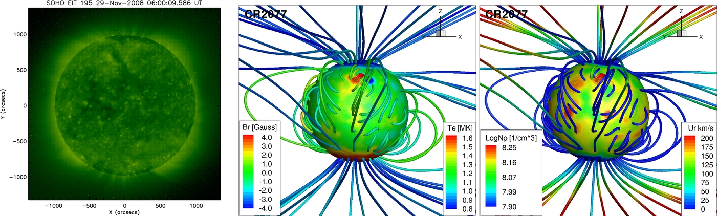
In Figure 1, a comparison between the SC output and SOHO/EIT observation is shown. The left image in Figure 1 shows the EIT 195 Å observation on 2008 November 29. In general, the Sun is very quiet except for a weak active region close to the north pole (without AR number). A large disk coronal hole region can be seen clearly around the equator, which extends to high latitude in the northern hemisphere. The middle and right images in Figure 1 show the SC output for the radial magnetic field and proton density at r = 1.055 R_☉ with selected field lines. For the radial magnetic field image, the field lines are colored by the electron temperature. We can see that the 3D topology of the solar magnetic field near the surface at solar minimum is characterized by open magnetic flux with lower temperatures at the two polar coronal hole regions and closed magnetic field lines with higher temperatures in the low latitudes. The active region can generate hot coronal loops. The existence of on-disk coronal holes (including polar and low-latitude coronal holes) is one of the major features of the SC during solar minimum (see review paper by Cranmer 2009). Therefore, the comparison of on-disk coronal holes between the observation and model is helpful for the model validation. In the right image of Figure 1, we show the proton density at r = 1.055 R_☉. The on-disk coronal hole regions shown in EIT 195 Å image can be seen as the low-density regions in the model output. The field lines of the right panel are colored by radial solar wind velocity, which suggests that the fast solar wind mainly comes from polar open field line regions and the slow solar wind originates near the solar equator. In general, the model output near the Sun reproduces many observed features.

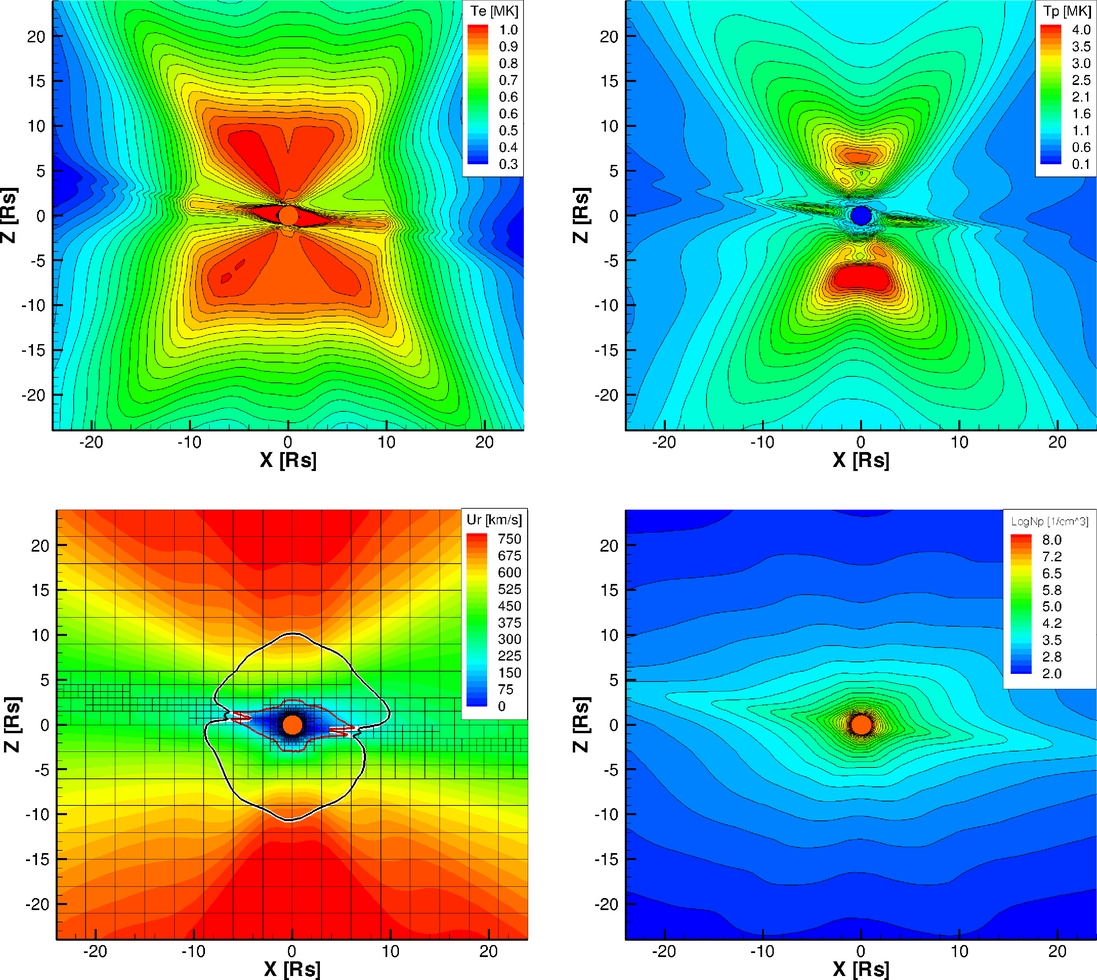
Zoom In Zoom Out Reset image size

In Figure 2, the meridional slice of the SC (−24 R_☉ ⩽ (x, y, z) ⩽ 24 R_☉) shows the electron temperature (top left), proton temperature (top right), radial solar wind velocity (bottom left), and proton density (bottom right). The model output without electron heating can be found in Figures 5 and 6 in van der Holst et al. (2010). Both the electron and proton temperatures are increased from van der Holst et al. (2010) model due to the change of the magnetic strength at the inner boundary. The electrons and protons near the Sun are in temperature equilibrium due to the Coulomb collisions. With the decrease of the density away from the Sun, the collisions become infrequent, therefore the electron and proton temperatures become different. For the electron temperature, we can still see the high temperature (above 1 MK) in the streamer region due to the electron heat conduction. The most obvious difference of electron temperatures between the models with and without electron heating lies in the coronal hole region. Without electron heating, the electron temperature decreases due to cooling by the adiabatic expansion of the solar wind plasma. With electron heating, the electrons maintain a high temperature (∼ 1 MK) within ∼10 R_☉, which then gradually decreases. The proton temperature shows similar bimodal structure. Due to the dissipation of Alfvén waves, the protons are hotter in the fast wind than in the slow wind. The proton temperature reaches ∼4 MK at ∼5 R_☉. There is no evident change to the solar wind velocity after adding the electron heating. The fast wind at high latitude reaches 700 km s⁻¹ and the slow wind speed at low latitude is below 400 km s⁻¹. The square boxes in the velocity figure show the adaptive mesh blocks. The refinement is made near the Sun and at the heliospheric current sheet. From the proton density figure, that latitude is also the region with the highest plasma density.

Zoom In Zoom Out Reset image size

In the velocity map of Figure 2, we also show some critical surfaces calculated from the model. The white contour line shows the critical surface where the solar wind speed equals the poloidal Alfvén speed (the Alfvén Mach number is unity). We can see that the radius of the Alfvén critical surface is ∼10 R_☉ outside of the streamer belt. Within the streamer belt, due to the increased density, the critical surface location drops to ∼5 R_☉. The black and red contour lines show the two critical surfaces where solar wind speeds are the same as the fast and slow magnetosonic-wave speeds, respectively. From the three critical surfaces, we can see clearly the Alfvén and fast magnetosonic critical surfaces coincide with each other at the polar regions, which is due to the fact that Alfvén speed is larger than sound speed. Similarly at the equator, the Alfvén and slow magnetosonic critical surfaces coincide because Alfvén speed is smaller than sound speed. Our results can be compared with some previous studies (Keppens & Goedbloed 1999; Usmanov et al. 2000). The critical surfaces are very important for both theoretical and simulation studies. Beyond the critical surface, the inward propagating waves cannot exist due to the faster outward moving solar wind plasma. To further validate the critical surface results, we need observations nearer to the Sun. Future missions (e.g., Solar Probe⁴) could bring us more valuable information about this issue.

In order to evaluate the electron heating effect in the two-temperature model near the Sun, we compare the model output with electron heating to the electron temperature and density derived from EUV images of the Sun by using the DEMT method (Frazin et al. 2009; Vásquez et al. 2010). In general, the DEMT method uses a time series of EUV images under the assumption of no time variation and uniform solar rotation to derive 3D emissivity distribution in each EUV band. By local differential emission measure (LDEM) analysis, the 3D distribution of the electron density and temperature can be obtained. The DEMT method assumes the plasma is optically thin. In this study, we use three bands of EUV observation (171, 195, and 284 Å) from EUVI on the STEREO A and B spacecraft.

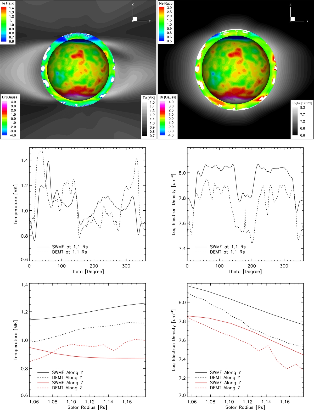
The top panels of Figure 3 shows the comparison between the model output and the DEMT-derived electron temperature (left panel) and number density (right panel) near the Sun. In both panels, the ring between r = 1.035 R_☉ and 1.225 R_☉ shows the ratio between the model and DEMT output. Outside this ring, the two-temperature model output is shown. At the center, the iso-surface of the Sun is taken at R = 1.055 R_☉ with the radial magnetic field shown on the surface. Some of the DEMT data points are set to zero due to the dynamic variation of the corona. These regions are marked by white. The temperature ratio is between ∼0.9 and ∼1.1 for most of the region. The relatively larger differences are shown outside the north polar region where the DEMT data shows two hot belts where the temperature is ∼40% hotter than the model. These two hot belts are associated with active regions, which our model (in its current form) cannot reproduce via Alfvén wave dissipation in closed field line regions. Due to the electron heating by the Alfvén waves dissipation, the electron temperature of the solar wind model increases in the coronal hole above ∼1 MK, which is also seen in the tomography. The ratio between the model and DEMT density is ∼0–0.3 in log scale (∼1–2 in normal scale) for most of the region. In the middle and bottom panels of Figure 3, we show the temperature and density curves at 1.1 R_☉ as well as along the Y- and Z-axes. This demonstrates that the electron heating is sufficient and the density scale height reproduces the observations.

Zoom In Zoom Out Reset image size

Although the results suggest a quantitative agreement between the model output and DEMT reconstruction, the assumptions of DEMT make it difficult to evaluate the accuracy of the results. First, DEMT used 3/4 of a Carrington rotation's data to reconstruct the density and temperature maps, while assuming no dynamic evolution of the corona. Also DEMT assumes a fixed iron abundance, to which the derived electron density is inversely proportional. In this work, we assume [Fe]/[H] = 1.26 × 10⁻⁴, which is four times higher than the photospheric value (Grevesse & Sauval 1998) due to the low first ionization potential (Feldman et al. 1992). The derived electron temperature is not affected by this caveat, but by the assumed ionization equilibrium fractions of the Fe ions. In the DEMT results here included (Vásquez et al. 2010), we used the ionization equilibrium calculations by Arnaud & Raymond (1992) to compute the EUVI bands' temperature responses. Therefore, we need further observational data to compare with and validate our model output. To achieve this, we use the spectral observation from the EIS on board Hinode to derive the electron density and temperature for a certain location and time during CR2077 and compare the result with model and DEMT output.

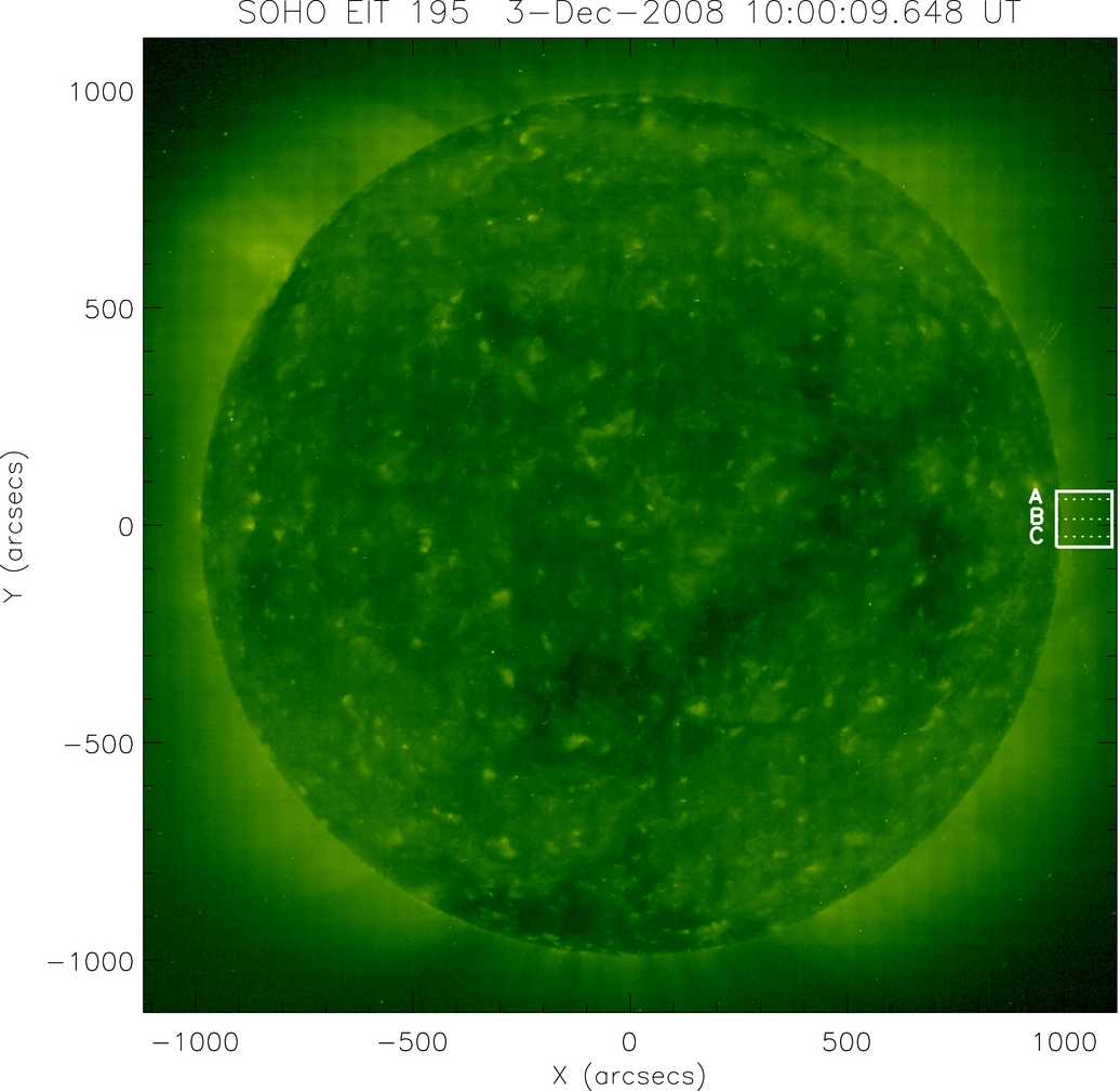
The west limb was observed on 2008 December 3 by the Hinode/EIS. A description of the EIS instrument can be found in Culhane et al. (2007). The observations were carried out using the 1'' slit and the central 128'' of the EIS detectors were downloaded. The EIS pointing was moved along the E–W direction 128 times with 1'' steps, so that the nominal field of view was 128'' × 128''. For each pointing, an exposure time of 90 s was used. The entire wavelength range of each EIS channel was downloaded, resulting in a full solar spectrum in the 166–212 Å and 245–291 Å wavelength ranges for each pointing. The center of the slit was pointed at (1025'', 14'') and a tiny portion of the limb was included in the field of view. Figure 4 shows the EIS field of view at three different temperatures using lines from He ii (formed at T ≃ 50,000 K), Fe viii (formed at T ≃ 400,000 K), and Fe xii (formed at T ≃ 1,500,000 K). The sharp decrease of the He ii intensity gives an approximate indication of the location of the solar limb; the intensity of all lines decreases exponentially beyond it. The data were reduced, cleaned, and calibrated using the standard EIS software available in SolarSoft. A wavelength-dependent shift along the N–S direction was applied to the images to account for the CCD spatial offset of the images; this was also calculated using the standard EIS software.

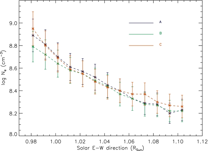
Zoom In Zoom Out Reset image size

Figure 4 shows the EUV image observed by SOHO/EIT on 2008 December 3. The white box shows the EIS field of view. The EIS observation suggests that the field of view is quite unstructured at transition region (i.e., Fe viii) temperatures, but shows two brighter areas and a darker lane at coronal temperatures. We have thus selected three data sets ("A," "B," and "C") to carry out the analysis, each including one of these features, and averaged the observed emission along the N–S direction at each position in the E–W scan. The position of the these three regions are marked by white dashed lines in Figure 4. The resulting data set consisted of three series of full EIS spectra as a function of height. The signal to noise becomes so low above 1.08 R_☉ that line intensities are too uncertain to derive physical properties of the emitting plasma. We are also interested only in data above 1.02 R_☉, to match the lowest height reached by tomographic reconstructions. We thus studied the spectra in the 1.02–1.07 R_☉ range only.

We measured the plasma electron density and thermal structure applying standard diagnostic techniques to EIS spectral line intensities. We measured the electron density using line intensity ratios, while we determined the plasma distribution with temperature for each region at each height by measuring the so-called differential emission measure (DEM) of the plasma using the iterative technique developed by Landi & Landini (1997). In our analysis, we used Version 6.0.1 of the CHIANTI database (Dere et al. 1997, 2009) and calculated the line emissivities adopting the ion fractions of Bryans et al. (2009) and the coronal abundances from Feldman et al. (1992).

Several ions provide line intensity ratios that can be used to measure the plasma electron density. However, signal to noise limited the maximum height where each ratio was able to provide meaningful electron density measurements. The Fe xii 186.8/195.1 intensity ratio proved to be the less noisy and allowed us to determine the electron density throughout the entire range of heights spanned by the observations. Figure 5 shows the results that the electron density decreases exponentially with height, and no significant difference is observed between the three regions. If we assume that the plasma is plane parallel and in hydrostatic equilibrium, the rate of density decrease in the 1.02–1.07 R_☉ range corresponds to a plasma electron temperature of T ≃ 3.8 × 10⁶ K, significantly larger than typical quiet Sun coronal temperatures (Phillips et al. 2008, and references therein).

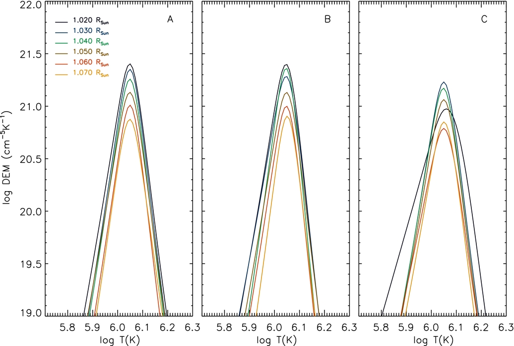
Zoom In Zoom Out Reset image size

The plasma DEM curves were measured for all three data sets and the results are shown in Figure 6. There are a few comments to the results. First, all three regions show qualitatively the same plasma distribution, although region C has slightly lower DEM curves. Second, all DEM curves are peaked around log T = 6.05, with a full width at half-maximum Δlog T ≃ 0.07: the plasma along the line of sight (LOS) is rather tightly clustered around the peak temperature. The DEM peak temperature is a factor ≃ 3 lower than the temperature derived by the density scale height. Third, the DEM peak values decrease monotonically with height, but they do not significantly change their shape, with the only exception being the curve at 1.02 R_☉ in the C data set.

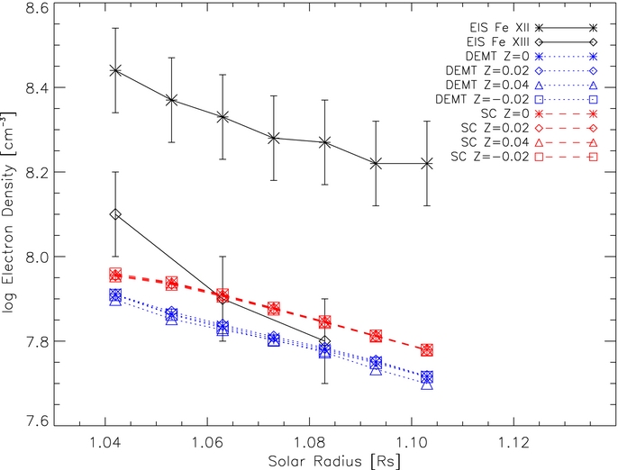
Zoom In Zoom Out Reset image size

To compare the electron density obtained by EIS, DEMT, and the model, we extract the LOS density at several locations around the B data set in the EIS observation for different solar radii from 1.042 to 1.103 R_☉. For the EIS observation, we show both the density derived from Fe xii and Fe xiii. The comparison result is shown in Figure 7. Since the location of EIS observation is the quiet Sun region, there are no significant differences at different locations for the densities predicted by the SC model and DEMT. The densities provided by SC and DEMT are very close as already shown in Figure 3. However, the density derived from EIS Fe xii is higher than the model and DEMT density by a factor of ∼2, while the density derived by the Fe xiii ratio is in good agreement. The disagreement between Fe xii and Fe xiii derived by EIS ratios was noted in previous studies (Young et al. 2009; Watanabe et al. 2009). In all cases Fe xii densities were higher than Fe xiii ones. The comparison made in this study shows that the Fe xiii-derived densities are more consistent with model and DEMT than Fe xii-derived densities. The agreement between the Fe xiii and DEMT density values, obtained with different techniques, reinforces the conclusion drawn by Young et al. (2009) and Watanabe et al. (2009) that Fe xii line intensities are affected by atomic physics problems. The EIS-derived temperature is around log T = 6.05 for all locations, which is well matched with the model output in Figure 3.

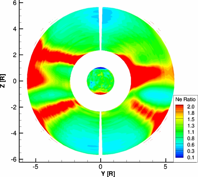
Zoom In Zoom Out Reset image size

As the final evaluation of the two-temperature model near the Sun, we compare the model result with the tomography derivation (Frazin 2000; Frazin & Janzen 2002) from SOHO/LASCO-C2. Using the LASCO-C2 observation, the tomographic method can obtain the electron density between 2.3 R_☉ and 6.0 R_☉. The electron density ratio between the model and the LASCO-C2 tomographic output is then calculated and shown in Figure 8. The data near ∼6.0 R_☉ are eliminated due to the relatively larger uncertainty of the tomography derivation near the boundary. In Figure 8, we can see that most of the regions have model/C2 ratio around 1.0, which means the model and C2 tomographic data are well matched. The four red streams that have a high model/C2 ratio are related to the time variation on the Sun that cannot be well captured by the steady-state solar wind model as well as the solar rotational tomography.

Zoom In Zoom Out Reset image size

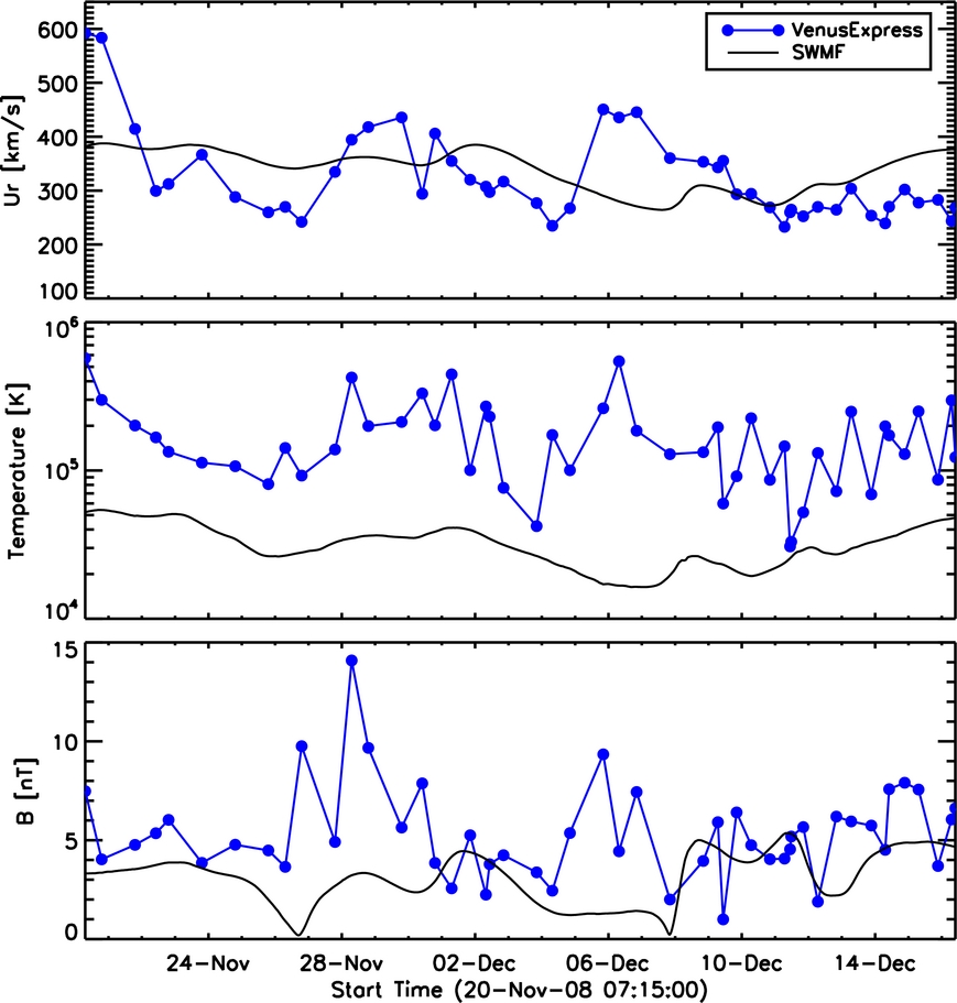
In this section, we will use multispacecraft observation from Venus Express (Titov et al. 2006), STEREO A/B, and ACE to validate our two-temperature model with electron heating in the heliosphere. Figure 9 shows the trajectories of the four spacecraft in the Carrington coordinate system (heliographic rotating coordinate, HGR).⁵ We can see that in the frame rotating with the Sun, the satellite trajectories encircle the Sun in a full Carrington rotation period. Venus Express is at ∼0.7 AU from the Sun. The other three satellites are at ∼1 AU. In Figure 9, three velocity iso-surfaces from the model are also shown. These three iso-surfaces show the radial solar wind speed of 250 km s⁻¹, 500 km s⁻¹, and 700 km s⁻¹, respectively. The corotating interaction regions (CIRs) that have been studied for several decades (see e.g., Jian et al. 2006; Mason et al. 2009, and references therein) are evident in our simulation results. In Figure 9, the CIRs are shown by the iso-surface velocity of 250 km s⁻¹, which are the slow streams. Figure 10 shows the comparison of the model with Venus Express observations at ∼0.7 AU. The proton parameters (solar wind speed and proton temperature) are observed by the Ion Mass Analyzer of the Analyzer of Space Plasma and Energetic Atoms on board Venus Express. The magnetic field strength is obtained by the magnetometer (MAG) on board Venus Express. Since solar wind monitoring is not a goal of Venus Express, the instruments on board Venus Express are switched on one hour before bow shock crossing and switched off one hour after. In this study, in order to exclude the influence of the atmosphere of Venus on the solar wind, we only use the first data point after switch on and the last data point before switch off. For the solar wind speed, the model agrees with the magnitude of ∼400 km s⁻¹, but differs in the speed variation. For the temperature, the model produces the same trend as the observation but with lower magnitude. The possible reasons for the discrepancy have been discussed by van der Holst et al. (2010). We will discuss it further in Section 4. For the magnetic field strength, both the model and observation give the same magnitude ∼5 nT.

Zoom In Zoom Out Reset image size

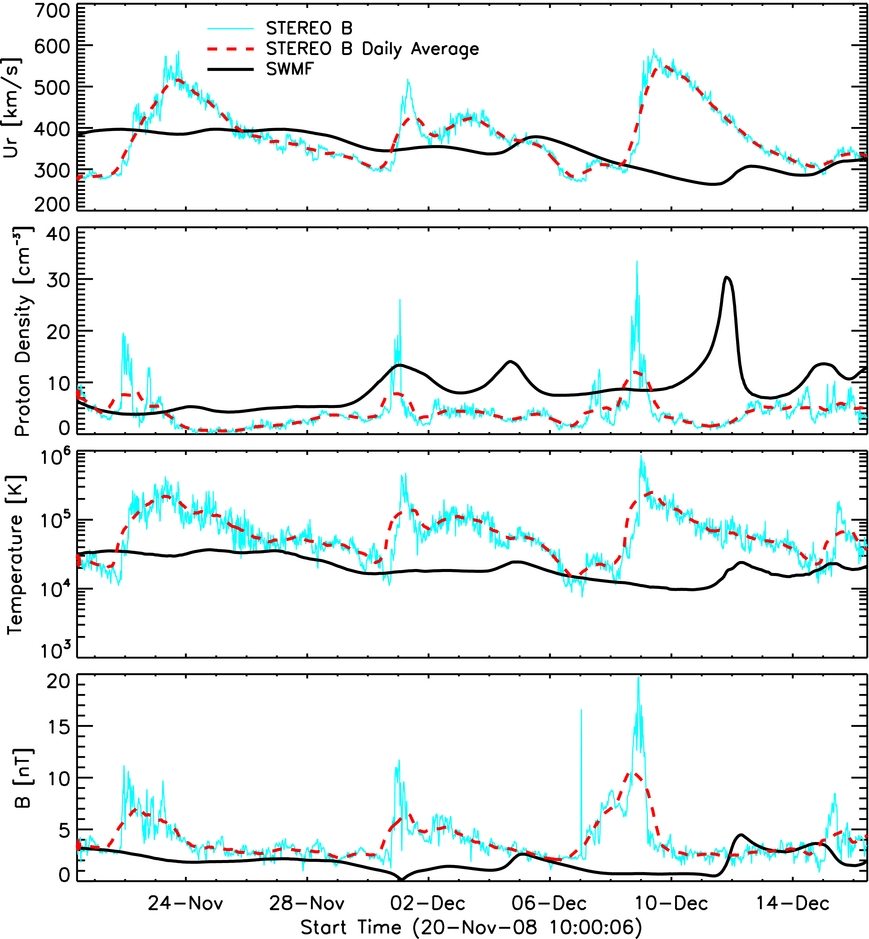
Zoom In Zoom Out Reset image size

Figure 11 shows the comparison between the model and the STEREO A observation. The proton parameters are observed by the Plasma and Supra-Thermal Ion Composition Investigation instrument on board STEREO. The magnetic field data is provided by the In-situ Measurements of Particles and CME Transients instrument onboard STEREO. The cyan lines in the figure show the original observational data with a time resolution of 10 minutes. There are many fine structures that cannot be captured by the steady-state MHD solutions. In order to compare the model output with the observation, a daily average of the observational data is shown with red dashed lines. In general, our model agrees to within a factor of two with STEREO observations in all the comparison parameters but some peaks are missing in our model. Some of these peaks might be related to eruptive events in the heliosphere that cannot be simulated by the steady-state solar wind model. Similar results are shown in Figure 12 for the comparison between the model and STEREO B observations.

Zoom In Zoom Out Reset image size

Zoom In Zoom Out Reset image size

Figure 13 shows the comparison between the model and ACE observations. We use the hourly averaged ACE data obtained from the Coordinated Data Analysis Web. Such a validation with ACE was also demonstrated by van der Holst et al. (2010) using the two-temperature model without electron heating. Comparing results, the model with electron heating can get similar features (e.g., CIRs) but with a higher magnitude, which is more consistent with the observations. We can see that the simulated solar wind speed has a peak above ∼400 km s⁻¹ and an average ∼350 km s⁻¹. The average proton temperature at 1 AU is higher and in better agreement with the ACE average temperature than the previous model presented in van der Holst et al. (2010), but several temperature peaks from the ACE data are no longer captured.

Zoom In Zoom Out Reset image size

We next use the freeze-in code developed by Gruesbeck et al. (2011) to calculate the ion charge state at 1 AU for the solar wind model, which we then compare to the observed values found by ACE/SWICS. As the solar wind plasma propagates outward from the Sun, the density significantly drops, which shuts down the ionization and recombination processes causing the freeze-in of the ionic charge state very close to the Sun. Lighter elements freeze-in closer to the Sun, while heavier elements freeze-in further out (Geiss et al. 1995; Buergi & Geiss 1986). Esser et al. (1998) first presented a model of ion charge state in the solar wind by solving the ionization evolution equations. Recently, Laming (2004) and Laming & Lepri (2007) suggested a model to interpret the increased ionization of charge states in the fast solar wind. The freeze-in code uses the solar wind model's electron temperature and density as inputs to the ionic charge state equation, while the model velocity is input into the continuity equation, which is solved for the plasma trajectory along a field line in the fast wind. The freeze-in code solves this series of equations using a fourth-order Runge–Kutta scheme, optimized for solving stiff sets of equations. The code is applied to separately calculate the charge state distribution of each atomic species as it propagates away from the Sun at the speed of the bulk velocity determined by the solar wind model. The ionization and recombination rate coefficients of specific ions are taken from Mazzotta et al. (1998).

The model's predicted freeze-in heights for C, O, Si, and Fe are approximately 1.13 R_☉, 1.13 R_☉, 1.45 R_☉, and 1.51 R_☉, respectively, illustrating the trend that has been theorized. As can be seen in the Figure 14, there is a strong qualitative agreement between the ACE/SWICS observations from a fast wind stream and the freeze-in code's results from the fast wind of the model. For all four elements inspected, the major charge state peak matches that of the ACE observation. The close match indicates that the model's coronal electrons temperature, density, and velocity are close to that of the SC. To determine the nature of the electron temperature discrepancy between the predicted and observed charge state levels is beyond the scope of this work, but will be taken up in subsequent papers. Also, we notice that the freeze-in heights for C and O are very close to the inner boundary of the simulation domain. Therefore, in order to have a more reliable result for these two elements, we may need to extend the inner boundary to the lower coronal region.

Zoom In Zoom Out Reset image size

We performed a validation study for the new 3D solar wind model (van der Holst et al. 2010) using observations of CR2077 from STEREO A/B, ACE, Venus Express, Hinode, and SOHO. We include electron heating in the new model by partitioning 40% of the Alfvén wave energy to the electrons. By comparing the model output with the DEMT electron temperature and density, LASCO-C2 tomographic density, and Hinode/EIS electron density and temperature, we suggest the model with electron heating is more physically reliable and consistent with observations than a single fluid model. The simulation results near the Sun reproduce many observational features (e.g., the open and closed field regions, low- and high-density regions, the fast and slow solar wind, and streamer belt) and get all the plasma parameters with the right magnitude (within a factor of ∼2).

Using the in situ observations from STEREO, ACE, and Venus Express, we compare the solar wind velocity, proton density, temperature, and magnetic field in the IH with the model output. In general, the validation results for CR2077 are encouraging. The heliosphere observational features (e.g., CIRs) are demonstrated in the simulation: The new model with electron heating also gets the right value of the solar wind speed, proton density, and the magnetic field strength for all of the in situ observations. Moreover, we validate the model with derived ionic charge states at 1 AU by using the newly developed freeze-in code by Gruesbeck et al. (2011). Our results show that the temperature profile of the model near the Sun can reproduce the ionic charge state observed by ACE/SWICS, which suggests the physical reliability of the new model.

However, there is still room for the improvement of the model. From the in situ observations, we notice that our model output has a relatively low magnitude at most CIR peaks for solar wind speed, density, temperature, and heliospheric magnetic field. The reason for this discrepancy is the quite extended slow wind region shown in Figure 2. This extended slow wind region positions the satellites in the slow wind for a longer period than occurred in reality and therefore causes the relatively low magnitude of plasma parameters. The wide slow wind region is caused by the difficulty of using the WSA model to obtain the Alfvén wave energy at the inner boundary in order to reproduce the final velocity distribution at 1 AU. The Alfvén wave pressure prediction is determined along the PFSS magnetic field, while the final obtained field line topology of the solar wind model departs from this PFSS field so that the velocity profile at 1 AU is likely to be different from the WSA predicted values. Actually, some studies found the WSA model yields higher solar wind speed at the source surface than the MHD model does (Feng et al. 2010). To overcome this issue, we may need a self-consistent method to treat the inner boundary for Alfvén wave energy. An improved solar wind model in SWMF will start from the top of the chromosphere and will be independent of WSA for the terminal solar wind speed. Also, including couterpropagating Alfvén waves (e.g., Chandran & Hollweg 2009; Cranmer 2010) may improve the heating and acceleration of the solar wind plasma.

In this validation study, in order to compensate for the uncertainty of the synoptic magnetogram observation and get the right magnetic strength at 1 AU, we double the magnetic field of the GONG-based synoptic magnetogram. How to create reliable and precise global solar magnetograms is still an open issue. With more observations from space by different satellites (e.g., Solar Dynamics Observatory (SDO), high temporal and spatial resolution; Solar Orbiter, polar region magnetic field measurement), as well as the development of new methods (e.g., helioseismology; Zhao 2007), the model can be improved by using more precise magnetograms.

There are also some ongoing DEMT improvements that include: (1) removing scattered light within the EUV telescopes, which is particularly important for fainter features such as the off-limb, coronal holes, and filament cavities; (2) including the Bryans et al. (2009) ionization fractions, which will imply changes in derived DEMT temperatures, especially in the hotter streamer regions. The new computation will change the EUVI responses and shift their peak location to higher temperatures. Therefore, the mean electron temperature from the inverted LDEM will also increase. For the Te > 1 MK regions, the median increase of the temperature is ∼15%, which could result in a better agreement between the two-temperature model and DEMT output; and (3) extending the technique to incorporate the SDO/Atmospheric Imaging Assembly (AIA) data, which provides more extensive temperature constraints than EUVI. Currently, a comparative study of EUVI and AIA-based DEMT results is being conducted for the current rising phase of solar cycle 24.

For future work, we need to validate the new SC model for solar maximum conditions. There are two difficulties for simulating solar maximum. First, the SC at solar maximum is more dynamic, which makes the boundary conditions based on potential field model and DEMT data less accurate. We also need to initiate CME events from different active regions in order to compare with observations. Moreover, our model does not take into account the coronal heating mechanism by ohmic dissipation associated with magnetic reconnection of which interchange reconnection is one example. Since interchange reconnections occur frequently during solar maximum, we need to see how it will influence our simulation results. Also note that a complete description of coronal electrons requires a kinetic treatment that can address the suprathermal electrons that are observed in situ. Furthermore, the core population has a nearly constant temperature of 100,000 K at 1 AU, which requires additional heating mechanisms for our model to reproduce. After the validation work, we will start to simulate eruptive events including CMEs and CME-driven shocks. In the previous solar wind model (Cohen et al. 2007) in the SWMF, the CME-driven shocks are not well described due to the reduced adiabatic index. The new model uses γ = 5/3 globally. Therefore, improvements in modeling CMEs and CME-driven shocks can be expected. Furthermore, by coupling the coronal model with the flux emergence convection zone model (Fang et al. 2010) with the SWMF, we can achieve self-consistent CME simulations in the future.

B.v.d.H. and W.M. are supported by NASA LWS NNX09AJ78G. The work of E.L. is supported by the NNX10AM17G, NNX11AC20G, and other NASA grants. J.R.G. is supported by the GSRP program from grant NNX10AM41H. We are thankful for the use of the NASA Supercomputer Pleiades at Ames and its helpful staff for making it possible to perform the simulations presented in this paper.

This work utilizes data obtained by the Global Oscillation Network Group (GONG) program, managed by the National Solar Observatory, which is operated by AURA, Inc. under a cooperative agreement with the National Science Foundation. The data were acquired by instruments operated by the Big Bear Solar Observatory, High Altitude Observatory, Learmonth Solar Observatory, Udaipur Solar Observatory, Instituto de Astrofísica de Canarias, and Cerro Tololo Interamerican Observatory. The LASCO-C2 project at Laboratoire d'Astrophysique de Marseille is funded by the Centre National d'Etudes Spatiales (CNES). LASCO was built by a consortium of the Naval Research Laboratory, USA, the Laboratoire d'Astrophysique de Marseille (formerly Laboratoire d'Astronomie Spatiale), France, the Max-Planck-Institut für Sonnensystemforschung (formerly Max Planck Institute für Aeronomie), Germany, and the School of Physics and Astronomy, University of Birmingham, UK. SOHO is a project of joint collaboration by ESA and NASA.