


ABSTRACT
In this paper, we examine the mode of dynamo action in the implicit large-eddy magnetohydrodynamical simulation of solar convection reported upon in Ghizaru et al. Motivated by the presence of a strong and well-defined large-scale axisymmetric magnetic component undergoing regular polarity reversals, we define the fluctuating component of the magnetic field as the difference between the total field and its zonal average. The subsequent analysis follows the physical logic and mathematical formulation of mean-field electrodynamics, whereby a turbulent electromotive force (EMF) is computed by the suitable averaging of cross-correlations between fluctuating flow and field components and expressed in terms of the mean field via a linear truncated tensorial expansion. We use singular value decomposition to perform a linear least-squares fit of the temporal variation of the EMF to that of the large-scale magnetic component, which yields the components of the full α-tensor. Its antisymmetric component, describing general turbulent pumping, is also extracted. The α-tensor so calculated reproduces a number of features already identified in local, Cartesian simulations of magnetohydrodynamical rotating convection, including an αϕϕ component positive in the northern solar hemisphere, peaking at high latitudes, and reversing sign near the bottom of the convection zone; downward turbulent pumping throughout the convecting layer; and significant equatorward turbulent pumping at mid latitudes, and poleward at high latitudes in subsurface layers. We also find that the EMF contributes significantly to the regeneration of the large-scale toroidal magnetic component, which from the point of view of mean-field dynamo models would imply that the simulation operates as an α2Ω dynamo. We find little significant evidence of α-quenching by the large-scale magnetic field. The amplitude of the magnetic cycle appears instead to be regulated primarily by a magnetically driven reduction of the differential rotation.
Export citation and abstract BibTeX RIS
1. INTRODUCTION
The solar magnetic field is the energy source for the whole set of physical phenomena collectively known as "solar activity." While flux emergence is the primary driver on timescales ranging from minutes to months, on longer timescales of years to millennia solar activity is strongly modulated by the solar cycle, namely the cyclic variation of the Sun's large-scale magnetic component. This cyclic variation, characterized by polarity reversals approximately every 11 years, is believed to be powered by a magnetohydrodynamical dynamo process operating in the solar interior, within its convective envelope and possibly immediately beneath its interface with the underlying, stably stratified radiative core (r/R☉ ≃ 0.71, according to helioseismic inversions of the solar internal sound speed profile; see, e.g., Christensen-Dalsgaard 2002). A proper understanding of this dynamo process is thus justly recognized as a cornerstone of research into the myriad of manifestations of solaractivity.
For physical conditions characteristic of the solar interior, the solar dynamo is expected to be well described by the classical magnetohydrodynamical approximation (e.g., Davidson 2001; Goedbloed & Poedts 2004), a fusion of the hydrodynamical fluid equations and Maxwell's equations applicable to a non-relativistic, globally neutral, and collisionally dominated plasma obeying Ohm's law. The resulting set of nonlinear, coupled partial differential equations remains daunting, and in general can only be solved numerically. Simplified model formulations based on mean-field electrodynamics (e.g., Moffatt 1978; Krause & Rädler 1980; Rüdiger & Hollerbach 2004, and references therein) readily produce cyclic solutions for reasonable though largely ad hoc input parameters and key functionals such as the α-effect and turbulent diffusivity (for a recent review see Charbonneau 2010). However (and without at all diminishing their usefulness as descriptive models as well as thinking tools), the freedom to specify free functions, and the highly simplified treatment of the nonlinear interactions between flow and field, poses fundamental limits on the applicability of such models to the solar cycle.
Alternately, the dynamo problem can be tackled as a dynamically consistent simulation of thermally driven magnetohydrodynamical convection in a thick, stratified, and rotating spherical shell of electrically conducting fluid (Gilman 1983; Glatzmaier 1984). The resulting computational problem is quite challenging due to the turbulent nature of fluid motions in the solar convection zone, which generates a very wide range of spatial and temporal scales in the evolving flow and magnetic field. For many decades, the computational resources needed to capture dynamo action in a global simulation of the whole solar convection zone have kept this type of simulation at the forefront of computational fluid dynamics, a situation that persists to this day (see Miesch & Toomre 2009 for a review).
Following the development of a massively parallel version of the Glatzmaier (1984) simulation code by Clune et al. (1999), a reasonably turbulent regime could be attained. While such turbulent global MHD simulations of solar convection do produce a lot of magnetic fields (see, e.g., Brun et al. 2004), they often fail to produce magnetic fields well organized on large spatial scales and carrying a significant net hemispheric flux. Toward this end, the introduction of a stable fluid layer underlying the convection zone, where strong, persistent angular velocity shear can develop in a tachocline-like layer, has been shown to be conducive to the buildup of persistent large-scale magnetic fields (see Browning et al. 2006; Ghizaru et al. 2010; Käpylä et al. 2010); however, at higher rotation rates it appears that the buildup of large-scale magnetic fields can occur entirely within the convective envelope, without a tachocline (Brown et al. 2010, 2011).
Regular, solar-like cyclic activity has proven very hard to produce in such simulations. The groundbreaking simulations of Gilman (1983) and Glatzmaier (1984, 1985) did produce polarity reversals, but computing limitations restricted these simulations to mildly turbulent regimes, while the resulting spatiotemporal evolution of the large-scale magnetic field they produced was non-solar in a number of ways, notably the tendency for latitudinal migration of the large-scale magnetic field to take place poleward rather than equatorward. In the more turbulent, contemporary versions of these simulations, polarity reversals of large-scale magnetic field structures, have been produced for rotation rates five times that of the Sun (Brown et al. 2011), with the timing of these reversals markedly asynchronous across hemispheres. Miesch et al. (2011) also reported on the occurrence of a few polarity reversals in a variation on the simulations of Brown et al. (2011) operating now at the solar rotation rate. This simulation shows better synchrony across hemispheres, but again a tendency, albeit weak, for poleward migration of the large-scale magnetic component. Operating under an entirely different numerical framework, Käpylä et al. (2010) also obtained cyclic large-scale magnetic fields in a spherical wedge simulation spanning up to 120° in longitude, 67° in latitude, and including an underlying stable layer. Those cycling large-scale magnetic fields again are characterized by poleward propagation much as in Gilman (1983) and also show strong hemispheric asymmetries.
At this writing the turbulent simulations having produced the most solar-like cyclic large-scale magnetic fields are those presented in Ghizaru et al. (2010). Based on an MHD extension of the well-documented general-purpose hydrodynamical simulation code EULAG (Prusa et al. 2008; Smolarkiewicz & Szmelter 2009, and references therein), the simulation is based on the hydrodynamical model setup of solar convection described in Elliott & Smolarkiewicz (2002). The temporally extended simulation reported in Ghizaru et al. (2010) is characterized by a number of encouragingly solar-like features: (1) a well-defined axisymmetric large-scale magnetic field component, antisymmetric about the equatorial plane; (2) magnetic polarity reversals with a half-period of approximately 30 years, synchronous across hemispheres; (3) a strong (up to 0.3 T) toroidal component concentrated at the interface between the convecting and underlying stable layers, peaking at mid latitudes and showing a weak but clear tendency for equatorward migration as the cycles unfold; (4) a dipolar component, well aligned with the rotation axis and strongly peaked at high latitudes; and (5) a reasonably solar-like internal differential rotation, showing equatorial acceleration and vanishing rapidly at the core–envelope interface. The most glaring departures from the observed solar cycle are the cycle period, three times too long; the fact that the large-scale surface poloidal and deep-seated toroidal component oscillate essentially in phase, in contrast to the π/2 phase lag observed on the Sun; and the pole-to-equator contrast in surface angular velocity, too small by a factor of almost three.
We are currently engaged in a systematic numerical exploration of parameter space, in order to answer a number of pressing questions, notably (1) what sets the cycle period in the simulation; (2) why our simulation is producing well-defined, fairly regular cycles while the simulations of, e.g., Browning et al. (2006), by all appearances quite similar in overall design and turbulent regime, did not; and (3) how robust the cycles are to the manner in which convection is being forced and to the dissipation introduced via the numerical advection scheme. This is a long, tedious, and computationally demanding process, which could be greatly accelerated if the physical nature of dynamo action in these simulations could be pinned down with some degree of confidence. Accordingly, the purpose of this paper is to examine the mode of dynamo action in the one specific simulation run presented in Ghizaru et al. (2010), which has since been extended to 337 years of simulated time, in the course of which 11 polarity reversals have taken place. Our primary aim is to examine the degree (if any) to which dynamo action in this simulation can be described through turbulent effects described by mean-field electrodynamics, as embodied in the α-effect and turbulent pumping. An overview of the simulation is first presented in Section 2, after which we describe the procedure adopted to extract the components of the α-tensor, and what these turn out to look like in our simulation (Section 3). We then examine (Section 4) the degree to which large-scale dynamo action in the simulation resembles what one can observe in conventional mean-field dynamo models and examine the relative importance of turbulent induction of the toroidal component versus shearing of the large-scale magnetic component by differential rotation. We close Section 5 by summarizing our results and speculating on further improvements that could lead to a better reproduction of the observed characteristics of the solar cycle in this type of MHD simulation.
2. OVERVIEW OF THE SIMULATION
The purpose of this section is to give a description of the magnetic cycles developing in a temporally extended version of the global MHD simulations of solar convection reported upon in Ghizaru et al. (2010). This specific simulation provides the numerical data used in the remainder of this paper in our analysis of large-scale dynamo action.
2.1. Computational Model
A detailed presentation of our simulation framework and numerical integration scheme will be given in a forthcoming publication, so that what follows is meant as an overview. The simulation solves the anelastic form of the ideal MHD equations in a thick, gravitationally stratified spherical shell (0.62 ⩽ r/R☉ ⩽ 0.96) spanning 3.4 density scale heights and rotating at the solar rate Ω☉ = 2.69 × 10⁻⁶ rad s−1. The analytic equations governing momentum, energy, and induction evolution are written in symbolic vector form as
In the above expressions  and
and  are the flow velocity and magnetic field, respectively, and Θ is the potential temperature, effectively a measure of specific entropy (s = cpln Θ). The Lagrangian derivative is defined in the usual manner
These evolution equations are also subject to mass continuity and solenoidality constraint on  :
:


In the momentum equation (1), π' is a density-normalized pressure perturbation in which magnetic pressure and centrifugal forces have been subsumed. The basic state defining the background stratification is unmagnetized, rigidly rotating, isentropic, and satisfies hydrostatic balance with g∝r−2. Subscripts "o" refer to this basic state, with primes denoting deviations from a prescribed ambient state, assumed to be in global thermodynamic equilibrium, consistent with helioseismically calibrated solar structural models (e.g., Christensen-Dalsgaard 2002). In our simulation this ambient state (subscript "e") is defined through a combination of polytropes, with a polytropic index varying linearly with r in the stable layer from n = 3.0 at the base of the domain to n = 1.5 at the base of the unstable layer at r/R☉ = 0.718, and set to n = 1.49995 within the model's convection zone. Radiative diffusion, symbolized by  on the right-hand side of Equation (2), is expressed in terms of the potential temperature perturbation as
with κr the coefficient of radiative diffusivity, and To(r) the temperature profile associated with the isentropic basic state. Convection is driven through the Newtonian cooling term αΘ' in Equation (2), which forces the system toward the ambient state on a timescale given by the inverse of α (α = 2 × 10⁻⁸ s−1 for the simulation considered here). This procedure, borrowed from simulation of an idealized terrestrial climate (Held & Suarez 1994; Smolarkiewicz et al. 2001), is physically equivalent to imposing a heat flux through the fluid layer. The simulation of Ghizaru et al. (2010), subjected to the residual (perturbation) solar heat flux, is only weakly forced from the convection point of view. Ongoing simulations operating under different forcing regimes indicate that simulated large-scale dynamo behavior can be sensitive to details of the forcing. Such sensitivity is not at all unusual in a turbulent fluid system (Piotrowski et al. 2009).
For numerical implementation, the system of evolutionary Equations (1)–(3) is written as a set of Eulerian conservation laws—using mass continuity and solenoidality, Equations (5) and (6)—and recast in the geospherical coordinate system (Prusa & Smolarkiewicz 2003):
where

denotes the vector of prognosed physical (viz., measurable) dependent variables, and R symbolizes all right-hand-side terms in Equations (1)–(3), including metric forces. The quantity ρ* = Gρo combines the anelastic density and the Jacobian of coordinate transformation, and  is an effective flux transport term constructed using contravariant velocity
  associated with the actual curvilinear coordinates used. The Lorentz force term in Equation (1) as well as the induction terms in Equation (3) are written in fully conservative form that incorporate
  and
and  under the divergence operator; cf. Section III in Bhattacharyya et al. (2010). Furthermore, an auxiliary term of the form −∇π* is added to the right-hand side of the induction Equation (3), in order to compensate for the truncation error-level departures from
  , through the solution, at every time step, of the associated elliptical problem for the auxiliary potential π*. The solution of the resulting conservation laws proceeds as outlined in Ghizaru et al. (2010), following the established EULAG procedures (Prusa & Smolarkiewicz 2003; Prusa et al. 2008).
Viscous, thermal, and Ohmic dissipation are conspicuously absent on the right-hand side of Equations (1)–(3); indeed, with the exception of the radiative diffusion term appearing explicitly on the right-hand side of Equation (2), all dissipation is delegated to the non-oscillatory advection scheme MPDATA (Smolarkiewicz 2006) at the core of EULAG. In essence, the higher-order truncation terms of MPDATA provide an implicit turbulence model (Domaradzki et al. 2003; Margolin et al. 2006; Margolin & Rider 2007). The simulation analyzed in what follows is computed at relatively low spatial resolution (Nr × Nθ × Nϕ = 47 × 64 × 128), which permits long temporal integrations, yet the low dissipative properties of the underlying computational framework still yield a reasonably turbulent regime, with estimated Reynolds numbers of order 102 and magnetic Prandtl number of order unity.
Simulations typically use a static state as initial condition, with small velocity and magnetic perturbations introduced at t = 0. The integration proceeds at a fixed-size time step, specifically half an hour, for a grand total of some 6 × 10⁶ time steps for the simulation discussed in what follows.
2.2. Cycling Large-scale Magnetic Fields
Figure 1 shows a temporal sequence of the toroidal (zonal) magnetic component in the simulation, extracted on a spherical shell corresponding to the core–envelope interface (r/R☉ = 0.718 in the simulation), plotted in latitude–longitude Mollweide projection. From top to bottom, the sequence runs from one magnetic maximum to the next and is temporally centered on a polarity reversal (middle panel). Despite strong fluctuations in the magnetic field, a large-scale axisymmetric component antisymmetric about the equatorial plane is clearly apparent except at the time of polarity reversal. In fact, except for the obvious reversal of magnetic polarity, the magnetic field distributions at the top and bottom are remarkably similar, showing concentration at mid latitudes and comparable peak strengths (∼0.3 T) in both hemispheres. Polarity reversals occur through a gradual weakening of the large-scale axisymmetric magnetic component, with antisymmetry about the equatorial plane maintained reasonably well as the time of reversal is approached (t = 202.5 years), and establishing itself rapidly again once the next half-cycle starts to build up (t = 221.9 years).

Figure 1. Temporal sequence of the toroidal magnetic component extracted at the core–envelope interface (r/R☉ = 0.718) in the three-dimensional MHD simulation presented in Ghizaru et al. (2010), plotted in Mollweide projection. The sequence runs from top to bottom and covers a time interval corresponding to a half-cycle, temporally centered on a polarity reversal. The color scale codes the magnetic field strength in Tesla.(An animation of this figure is available in the online journal.)
Download figure:
Standard image High-resolution imageThe spatiotemporal evolution of the large-scale axisymmetric component is best viewed by zonally averaging the total magnetic field present at any given time in the simulation. Working in spherical coordinates (r, θ, ϕ), where −π/2 ⩽ θ ⩽ π/2 is the latitude (rather than the polar angle), such a zonal average is defined as
The top panel in Figure 2 shows a time–latitude diagram of the toroidal magnetic component (〈Bϕ〉) averaged in this manner, constructed at a depth corresponding to the core–envelope interface in the model (r/R☉ = 0.718). If the toroidal magnetic flux ropes assumed to give rise to bipolar active regions are indeed stored at this depth, as suggested by stability analyses (e.g., Ferriz-Mas et al. 1994; Fan 2009), and rise radially to the photosphere, then this is the simulation's equivalent to the sunspot butterfly diagram (e.g., Hathaway 2010). The toroidal magnetic component is concentrated at mid latitudes (30° ⩽ |θ| ⩽ 70°), as opposed to the low latitudes (5° ⩽ |θ| ⩽ 40°) suggested by the butterfly diagram, but does show a tendency for equatorial migration as each half-cycle unfolds. On a time–latitude diagram such as Figure 2 (top panel), this is seen in the strong toroidal field concentrations, which take an elongated, elliptical shape, with the "major axis" tilted toward the equator as the cycle is followed in time. In other words, throughout a cycle the latitude of the peak large-scale toroidal magnetic field occurs at decreasing latitudes, until the cycle terminates and the next one begins anew at higher latitudes.

Figure 2. Spatiotemporal evolution of the zonally averaged magnetic field in the three-dimensional MHD simulation of Ghizaru et al. (2010). Top panel: time–latitude diagram of the zonally averaged toroidal magnetic component at the core–envelope interface (r/R☉ = 0.718); middle panel: corresponding radius–latitude diagram, extracted at latitude −45° in the southern hemisphere. The dashed line indicates the core–envelope interface; bottom panel: time–latitude diagram of the zonally averaged surface radial field (r/R☉ = 0.96), with magnetic half-cycles numbered from each minimum to the next as with the sunspot cycles. The color scale codes the magnetic field strength in Tesla.
Download figure:
Standard image High-resolution imageThe middle panel of Figure 2 shows the time–radius slice of the same simulation run, extracted in the southern hemisphere at latitude −45°, where the toroidal field is strongest at the core–envelope interface (cf. top panel). Note how polarity reversals begin well within the convection zone, at depth r/R☉ ≃ 0.8, with radial drift and concentration of the magnetic field both upward as well as downward all the way to the core–envelope interface, where the field reaches its peak strength.
The bottom panel of Figure 2 shows the corresponding time evolution of the zonally averaged radial surface magnetic component, again in a time–latitude diagram. The surface field is characterized by a well-defined dipole moment closely aligned with the rotational axis, with transport of surface fields taking place from lower latitudes, and possibly contributing to the reversal of the dipole moment. Comparing the three panels in Figure 2 reveals that the dipole moment and deep-seated toroidal component reach their peaks at approximately the same time, indicating that they oscillate in phase, without significant temporal lag.
Overall, the magnetic cycle characterizing the large-scale, zonally averaged magnetic component is quite regular, here with a half-period of 30 years, almost thrice the 11 years of the solar cycle. Note the good long-term synchrony maintained between the northern and southern hemispheres, persisting despite significant fluctuations in the amplitude and duration of cycles in each hemisphere. In keeping with solar tradition, we delineate the cycles from one toroidal field polarity reversal to the next. Remember therefore that what we henceforth refer to as "cycle," as numbered on the bottom panel of Figure 2, spans in fact one-half of a complete magnetic cycle. While the average period of our cycles so-defined is almost exactly 30 years for our 11 cycles, this period can become as low as 25 years (simulated cycle 11) or as high as 35 (simulated cycle 4) from one cycle to the next.
2.3. Large-scale Flows
Stratification and rotation, the latter through the agency of the Coriolis force, introduce cross-correlation between turbulent velocity components that lead to significant Reynolds stresses powering large-scale flows throughout the solar convection zone. This phenomenon also arises naturally in the type of rotating, stratified convection simulations considered here, in either the hydrodynamical or magnetohydrodynamical regimes (e.g., Miesch et al. 2000; Brun et al. 2004; Browning et al. 2006, and references therein).
The zonal averaging procedure defined in Equation (10) can be used to extract a mean flow  from the simulation output. The result of this procedure is shown in Figure 3, in the form of isocontours of zonally averaged rotational frequency (angular velocity divided by 2π) and meridional flow vectors superimposed on a color coding of the latitudinal mean-flow component 〈uθ〉. This is a purely hydrodynamical parent simulation subjected to the same thermal forcing as the MHD simulation described above. Differential rotation is reasonably solar-like, with equatorial acceleration and near-radial isocontours at mid to high latitudes, transiting rapidly to rigid rotation across a thin tachocline-like shear layer located immediately beneath the convective layers. The sharpness of this rotational transition layer is noteworthy for these types of simulations; it is a direct reflection of the low dissipation embodied in our numerical scheme and of the rapidly increasing subadiabaticity with depth characterizing our ambient stratification. The pole-to-equator contrast in surface and subsurface rotation rate, ∼100 nHz, is also reasonably solar-like. This differential rotation pattern remains fairly steady over the time span of the simulation. The large-scale meridional flow, in contrast, is much more strongly fluctuating, but when averaged over a sufficient long time span, away from the equatorial regions the net flow is found to be poleward in the surface and subsurface layers, and equatorward near the base of the convection zone. The surface meridional flow, peaking at ∼1 m s−1 at mid to high latitudes, is about a factor of 10 slower than observed on the solar surface. At lower latitudes, the elongated flow structures parallel to the rotation axis are the residual signature of persistent elongated convective rolls stretching across the equator, typical of these types of simulations running in this turbulent regime (see, e.g., Miesch et al. 2000, Figure 5; Brun et al. 2004, Figure 1; Käpylä et al. 2010, Figure 2).

Figure 3. Zonally averaged angular velocity (left), and meridional flow (right) in a hydrodynamical simulation of solar convection ran in the same parameter and forcing regime as the MHD simulation presented in Figures 1 and 2. The angular velocity profile is solar-like, including in particular a thin, tachocline-like rotational shear layer straddling the interface between the convection zone and underlying stable layer (indicated by the dashed circular arc). The meridional flow vectors (right) are superimposed on a color coding for the magnitude of the latitudinal mean-flow component 〈uθ〉. While these plots were produced by averaging in time over some 100 years, the differential rotation is found to remain remarkably steady over the duration of the simulation. The meridional flow is more strongly fluctuating, but the vertically elongated flow structures crossing the equator are relatively steady, as they reflect the presence of quasi-steady, convective rolls, stacked in longitude and aligned with the rotation axis, and which yield a residual signature upon zonal averaging. They show up very prominently here because the meridional flow at mid to high latitude is much slower than convective velocities.
Download figure:
Standard image High-resolution imageTurning now to our MHD simulation, these large-scale flows are now found to carry the signature of the magnetic cycle. This is shown in Figure 4, displaying again the rotational frequency and meridional flow in meridional planes, in the same format and using the same color scales and ranges as in Figure 3, together now with the zonally averaged toroidal magnetic component (rightmost plots). These were all averaged in time over as temporal window of width Δt = 3.3 years, about one-tenth of a magnetic half-cycle, centered over the peak of simulated cycle 1 (t = 16 years, top row) and following cycle minimum (t = 32 years, bottom row). Differential rotation (left) is again characterized by equatorial acceleration, but there now remains little latitudinal gradients at mid latitudes as compared to the parent hydrodynamical simulation. The pole-to-equator contrast in rotation rates is down to 40 nHz at epochs of cycle minimum, and even less at maximum, which is now a far less solar-like situation. Differential rotation spreads somewhat deeper into the stable layer, especially at high latitudes, but a modest tachocline-like shear layer still persists. Significant cycle-driven torsional oscillations materialize throughout the simulation. In Figure 4, this is mostly apparent at high latitudes, with the polar region speeding up at time of cycle maxima, but lower-amplitude torsional oscillations are actually present also in equatorial regions and at all depths.

Figure 4. Zonally averaged angular velocity (left), meridional flow (middle) a toroidal magnetic component (right) at time of cycle maximum (t = 16 years, top row) and minimum (t = 32 years, bottom row). The zonal means were also averaged in time over a temporal window of width 3.3 years in order to produce smoother plots. The ranges of the color scales are deliberately kept the same as in Figure 3, so as to highlight the strong suppression of differential rotation as compared to the purely hydrodynamical parent simulation, and enhancement of the meridional flow at times of cycle maximum. Noteworthy cycle-induced variations in the axisymmetric flows include torsional oscillations superimposed on the differential rotation profile, and the development of secondary meridional flow cells at high latitudes (see the text).
Download figure:
Standard image High-resolution imageThe surface and subsurface meridional flow remains generally poleward at mid to high latitudes, although secondary, counterrotating flow cells develop in the descending phase of the cycles, their onset visible here on the 〈uθ〉 plot at maximum phase. At the base of the convecting layers, the meridional flow is equatorward at mid to high latitudes at all cycle phases, but does show significant cyclic variations in speed, generally being more vigorous near cycle maximum, reaching half a meter per second at ±60° latitude. The flow pattern near times of "cycle minimum" more closely resembles what is observed in the purely hydrodynamical simulation (cf. Figure 3).
2.4. Energetics
With zonal means of the total flow  and magnetic field
  defined through Equation (10), subtracting these means from the total flow and magnetic field then yields the non-axisymmetric contributions:


In the following section, we shall demonstrate that these non-axisymmetric contributions can be reasonably associated with small spatial scales and are henceforth referred to as such, while the zonal means can be associated with large spatial scales, commensurate with the size of the simulation domain. It is then straightforward to compute the contributions of these various flow and field components to the total specific energy budget, through volume averages over the full simulation domain:
with  , etc. The comparison between these various contributions is carried out pictorially in Figure 5, in the form of time series spanning the full simulation run. All four contributions are similar in magnitude, and the cycle stands out as a prominent, smooth cyclic variation in the energy contribution of the axisymmetric component of the magnetic field, which varies by a factor of 2–3 between epochs of cycle "maxima" and "minima." The small-scale magnetic energy E(B') does show some in-phase variations with E(〈B〉), but the energy contributions of the non-axisymmetric flow component, dominated by turbulent convection, remain remarkably steady in comparison, showing only short timescale fluctuations about a well-defined mean value. The energy contribution of the axisymmetric flow, dominated by differential rotation, shows variations on timescale commensurate with the cycle of the axisymmetric part of the magnetic field and reflects the signature of torsional oscillations.
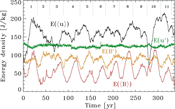
Figure 5. Time series of the four contributions to the global energy budget, as defined via Equations (13)–(16), as labeled. The 30 year cycle shows up prominently in E(〈B〉), as it of course should, and also in E(〈u〉) but more weakly in E(B') and hardly at all in E(u'). Note also how the large-scale flow and field are globally within a factor of two of energy equipartition at times of cycle maximum. Numbering of simulated half-cycles as in Figure 2.
Download figure:
Standard image High-resolution image3. MEAN-FIELD ANALYSIS
3.1. Scale Separation and Averages
Mean-field electrodynamics is predicated on the assumption that the fluid flow ( ) and magnetic field (
 ) can be separated into "mean" (usually spatially large-scale and slowly varying in time) and "fluctuating" (usually small-scale and rapidly varying) components:

where the angular brackets denote an intermediate averaging scale for which

Given the well-defined large-scale axisymmetric component present in our simulation, it becomes natural to associate the averaging scale with the zonal average defined through Equation (10), so that the fluctuating components become defined as the non-axisymmetric contributions through Equations (11) and (12). In practice, it is of course possible to define fluctuating flows and fields in this way for any global MHD simulation run. However, for the mean-field electrodynamics approach to be mathematically well-posed and physically meaningful, it is essential for a good separation of scales to hold. Accordingly, we first examine in some detail whether this is indeed the case for our simulation.
Figure 6 shows the mean and fluctuating toroidal magnetic field components resulting from this decomposition applied to the toroidal field distribution plotted on the bottom panel of Figure 1 (simulation time t = 230 years, very near the peak of simulated cycle 8). At the base of the convection zone, both components have similar strength, but the fluctuating component in Figure 6 shows little or no azimuthal structuring on scales comparable to the solar radius, nor any clear hemispheric pattern. In particular, no sign of a significant non-axisymmetric dipolar or quadrupolar components is visible.

Figure 6. Latitude–longitude Mollweide projection of the zonally averaged toroidal magnetic component (top), and associated small-scale fluctuating toroidal component (bottom), as defined by Equation (12), extracted at a depth corresponding to the core–envelope interface at simulation time t = 230 years, near the peak of magnetic half-cycle number 8 (see Figure 2). The sum of these two components is the total toroidal field distribution plotted on the bottom panel of Figure 1.
Download figure:
Standard image High-resolution imageThis visual impression is confirmed by a modal decomposition in spherical harmonics, which reveals significant power concentrated in the axisymmetric (m = 0) mode of low, odd angular degree ℓ. This is illustrated in Figure 7, showing the result of a modal decomposition of the toroidal magnetic component at the core–envelope interface (r/R☉ = 0.718). The decomposition was carried out at every time step and then averaged for two sets of disjoint data blocks of temporal width 900 days centered either on the epochs of polarity reversals (panel A, for "cycle minima") or peak toroidal field (panel B, for "cycle maxima"). The top row of Figure 7 displays the result of this procedure in the form of color coding of the absolute values of the modal coefficients, in the plane defined by the angular degree ℓ (horizontal) and azimuthal degree m (vertical). The diamond shape results from the truncation of azimuthal modes, chosen so as to ensure comparable peak spatial resolution in the latitudinal and azimuthal directions.

Figure 7. Spectral distribution of modal amplitudes for the toroidal magnetic component at the core–envelope interface in the simulation, r/R☉ = 0.718. The top row shows power distributions in the (l, m) plane. The unsigned values resulting from a standard spherical harmonic decomposition were averaged over two sets of disjointed blocks centered over cycle minima (panel A) and maxima (panel B), respectively. Panel C results from subtracting panel A from panel B and shows the amplitude distribution associated with the large-scale magnetic component, which is concentrated primarily in the (ℓ, m) = (1, 0) and (5, 0) modes. The color scale spans two orders of magnitude, in constant logarithmic increments, running from 5 × 10⁻³ to 0.67 T. The bottom plot shows, as a function of the latitudinal wavenumber ℓ, the power of all non-axisymmetric modes summed over the azimuthal wavenumber m (dotted lines), with the solid line corresponding to axisymmetric (m = 0) modes.
Download figure:
Standard image High-resolution imageComparing panels A and B of Figure 7 reveals significant power in the axisymmetric (m = 0) angular modes of odd-ℓ angular degree at cycle maximum that all but vanish at times of cycle minimum. This is particularly prominent for the dipolar (ℓ, m) = (1, 0) mode. At high-ℓ values, on the other hand, power is broadly and more evenly distributed in modes of all azimuthal orders m and shows no clear variations with the phase of the cycle for the large-scale field. Indeed, subtracting panel B from panel A, yielding panel C in Figure 7, reveals very little residual power at high wavenumbers.
Figure 7(D) shows the variation of the same (unsigned) modal coefficients as a function of the latitudinal wavenumber ℓ for the axisymmetric modes only (m = 0, solid lines), and the quadratic sum of all coefficients for non-axisymmetric modes ( , dotted lines). The latter are seen to dominate over the former for ℓ ⩾ 10, but are of comparable amplitude for smaller ℓ, except at maximum epochs (red lines) where the modal amplitudes are dominated by the ℓ = 1 and ℓ = 5 axisymmetric modes. Note also how the summed non-axisymmetric coefficients at maximum and minimum epochs (red and green dotted lines) are almost exactly coincident at all ℓ-values. For axisymmetric modes (solid lines), this holds only for ℓ ⩾ 10. In addition, the peaks at ℓ = 1 and l = 5 remain present at almost the same amplitude in the subtracted distribution (black), while the amplitude for other modes drops significantly, by over an order of magnitude at high ℓ-values. In fact, for axisymmetric modes the only significant difference between maximum and minimum phases is suppression of the ℓ = 1 and ℓ = 5 modal amplitudes. All this indicates that the cycle in the large-scale axisymmetric magnetic field does not alter significantly the spectral properties of the small-scale, "turbulent" magnetic component.
Examining time series of individual modal coefficients reveals that the cycle shows up prominently in the (ℓ, m) = (1, 0) and (5, 0) modes, but the time series for  modes, as well as for even-ℓ axisymmetric modes, have much lower amplitudes and show no sign of persistent cyclic variation. This has been further verified by computing Fourier transforms of these various time series, which show clear peaks at periods of ∼29 and ∼58 years in the odd-ℓ axisymmetric modes, but no peaks and overall power levels inferior by over an order of magnitude for even-ℓ and
  modes. Similar temporal patterns are observed within the convection zone and/or for the other magnetic components. Overall, the above analyses then suggest that the decomposition embodied in Equations (11) and (12) represents a viable ansatz, at least for this simulation run.
3.2. The Turbulent Electromotive Force
With the assumption of scale separation vindicated at least to some degree, our purpose is now to identify and characterize the dynamo mechanism underlying the observed magnetic cycle described above. The starting point of the analysis is the magnetohydrodynamical induction equation (e.g., Davidson 2001), describing the evolution of a magnetic field  subjected to the inductive action of a flow field
  in addition to Ohmic dissipation of the associated electrical current density:
where η = (μ0σe)−1 is the magnetic diffusivity, inversely proportional to the electrical conductivity σe (SI units are used throughout). Note that explicit Ohmic dissipation is now retained, unlike in the induction equation solved by the simulation (cf. Equation (3)). Inserting Equations (17) and performing the zonal average introduced earlier, and remembering that the averaging operator commutes with spatial derivatives pertaining to the large spatial scales, one readily obtains
where

is the mean EMF due to the fluctuations about the large-scale magnetic field. Note that this mean turbulent EMF is generally nonzero, because the correlation between the fluctuating flow and magnetic field does not necessarily vanish upon averaging, even though  and
and  individually do by definition. For more details on some of the many subtleties involved, see, e.g., Moffatt (1978), Rüdiger & Hollerbach (2004), Hoyng (2003), and Ossendrijver (2003).
From the simulation results, it is straightforward to reconstruct  and
and  via Equations (11) and (12), and then compute the EMF by performing the required cross product and zonal averaging at every time step, as per Equation (21). The result of this calculation is presented in Figure 8 for the r (top), θ (middle), and ϕ (bottom) components of the EMF, in the form of time–latitude slices at depth r/R☉ = 0.85 near the middle of the convection zone (left panels), where polarity reversals are initiated (see Figure 2), and meridional slices extracted at simulation time t = 112 years, at the peak of the fourth magnetic half-cycle (right panels). Note already how the EMF vanishes rapidly as one moves below the core–envelope interface, as expected since convectively driven turbulence disappears there. Otherwise the EMF pervades most of the convection zone. Despite being a very noisy "signal," on the largest spatial scales all EMF components exhibit a well-defined symmetry (
 ,
,  ) or antisymmetry (
 ) about the equatorial plane. Note in particular that a ϕ-component of the EMF positive (negative) in both hemispheres is precisely what is required to support a positive (negative) dipole moment (cf. bottom panels in Figures 2 and 8), as per the right-hand rule, since under the MHD approximation the EMF drives a parallel electrical current density. Moreover, reversing the direction of this EMF every half-cycle then amounts to reversing the sign of that dipole moment, as observed in the simulation.

Figure 8. Three components of the turbulent EMF  . The left column shows time–latitude slices extracted at the middle of the convection zone (r/R☉ = 0.85), while the right column shows snapshots of the spatial variations in meridional planes, at the peak of simulated cycle 4 (t = 112 years). For the purpose of constructing the time–latitude diagrams, the simulation was undersampled at intervals of 10 solar days (≃ 0.82 years).
Download figure:
Standard image High-resolution imageAll EMF components show strongly reduced amplitudes in the equatorial regions. This can be traced to a change in the topological character of convective fluid motions, which at low latitudes tend to organize themselves in longitudinal stacks of large, latitudinally elongated convective cells approximately aligned with the rotational axis (see Figure 1(A) in Ghizaru et al. 2010). These are quite typical of these types of global convection simulations (see, e.g., Browning et al. 2006, Figure 1; Brown et al. 2010, Figure 1; Käpylä et al. 2010, Figure 2). Evidence of a quenching of the small-scale flow components can also be found in the spatial distribution of the small-scale surface magnetic field, which shows a significant decrease in both coverage and magnitude at very low latitudes (see, e.g., Figure 1(B) in Ghizaru et al. 2010).
The most striking global spatiotemporal feature visible in Figure 8 is certainly the cyclic variation of all EMF components, with a period identical to that of the cycle observed in the large-scale magnetic field (cf. Figure 2). Here the large-scale velocity field is roughly stationary over the entire simulation, and the small-scale turbulent velocity field is also stationary in a statistical sense (cf. Figure 5). Since the EMF term depends only on the small-scale fluctuations about the large-scale magnetic fields, it is then not at all obvious a priori that the EMF should exhibit the same cyclic evolution as the mean field; the fact that it does already provides us with important clues as to the nature of the large-scale dynamo operating in our simulation. More specifically, it suggests that the turbulent EMF actually plays a key role in the production of the large-scale magnetic component. We now turn to this question, using the mathematical machinery of mean-field electrodynamics.
3.3. The α-tensor
The essence of mean-field electrodynamics is to provide an expression for the EMF in terms of the large-scale magnetic field, so that the small scales (fluctuations) are effectively removed from the problem. The procedure consists of a simple linear expansion of the EMF as a power series about the large-scale magnetic field and its derivatives, i.e.,

with summation implied over repeated indices. The tensors appearing on the right-hand side of this expression and relating the EMF to the mean field can depend on the properties of small-scale flow and field fluctuations, but not on the mean field itself, a situation expected to hold only if the latter is too weak to impact the dynamics of the fluctuating flow. Even though it is defined globally, the steadiness of the time series of the energy contribution of the small-scale flow on the temporal scale of the cycle in the large-scale field, as seen in Figure 5, is consistent with this working hypothesis. Note also here that since this expansion is linear in the large-scale field, if that field exhibits cyclic properties, then so should the EMF, which is what we observe (cf. Figure 8). This is our central motivation for appealing to mean-field electrodynamics to analyze the dynamo operating deep in the convection zone of our simulation.
The leading-order contribution in the right-hand side of Equation (22) is usually named the "α-effect." The second term in the expansion is responsible, among other effects, for turbulent diffusion. For our first analysis, however, we retain only the α-effect for simplicity. Owing to the rough stationarity of the large-scale flows in the simulation, we also assume that αij is time independent, an assumption that will prove itself well-verified a posteriori. We thus write as a first approximation

One can further decompose αij into symmetric and antisymmetric parts, such that the EMF may be rewritten as

where
is called the general turbulent pumping velocity, because it effectively provides an additive contribution to the mean, large-scale inductive flow in Equation (20), although its physical origin lies with the fluctuating, small-scale flow and magnetic field. The flow-like vector field  so-defined is in general non-solenoidal (
 ) and acts on the total magnetic field, with variations between magnetic component subsumed into the off-diagonal terms of the symmetric part of the α-tensor (see Ossendrijver et al. 2002 for a more thorough discussion).
3.4. Extracting the Components of the α-tensor
A number of methods have been designed to measure the components of the α-tensor in turbulent MHD simulations (e.g., Ossendrijver et al. 2001, 2002; Käpylä et al. 2006, 2009; Hubbard et al. 2009, and references therein). These method have been designed in the context of MHD simulations that do not produce a well-defined large-scale magnetic component, so that the latter must be imposed externally—and artificially—with the consequence that the α-tensor being measured is not necessarily characterizing the simulation prior to the application of the external field. For more on these—and other—difficulties, see Brandenburg (2009), Cattaneo & Hughes (2009), and references therein. In contrast, we are in the very advantageous position to have in hand a simulation that does generate a large-scale magnetic field, in a manner consistent with the dynamical interaction of flow and field on all numerically resolved spatial scales.
The procedure we employ here to extract αij from the simulation data differs from the approaches found in the literature, and we shall therefore first detail it. Essentially, we attack this problem from an experimentalist's point of view, i.e., we have (numerical) data in our possession, namely the EMF and the average magnetic field, and we wish to verify if these data match a specific model, namely the α-effect parameterization of the EMF embodied in Equation (23). This task therefore amounts to a fitting problem, in other words the components of the tensor αij are calculated a posteriori by minimizing the difference between the left-hand side and right-hand side of Equation (23). We opt here for a standard least-squares fit, based upon singular value decomposition (hereafter SVD; see Press et al. 1992, Section 15.4). We state results of various theorems without proof.
For a given component, say m (=r, θ or ϕ) of the EMF at a fixed grid point4 (rb, θc), we define the time-dependent functions y(t) and Xk(t) as follows:


We also define

which then allows us to rewrite the parameterization of the EMF as
Denoting by Nt the number of time steps of our simulation, we define a merit function as
where ti is the value of the time coordinate at the ith step. The goals are to find the three parameters ak that minimize the merit function and to obtain an estimate of the goodness of fit. The method we employ to carry out these two tasks simultaneously is the SVD of the "design matrix"  , defined as

The design matrix therefore depends on the large-scale magnetic field components. This matrix has Nt rows and three columns, and by virtue of a theorem of linear algebra, can always be decomposed as follows:

where the matrix  is an nt-by-three column orthogonal matrix,
  is a three-by-three diagonal matrix containing the so-called singular values, and
  is a three-by-three orthogonal matrix. The key element is that the solution to the minimization of the merit function (29) is directly obtained in terms of the three matrices
  ,
,  and
and  . The solution vector
  is given by

where the vector  and therefore depends on the selected EMF component. To construct the SVD of our design matrix, we use the algorithm and routines of Press et al. (1992), as implemented in the IDL programming language. By repeating this procedure for all three components of the EMF and for each of the Nr × Nθ grid points (rb, θc), we can calculate the complete tensor αij(r, θ).
Figure 9 shows the results of this fitting procedure over the complete 337 year simulation interval. Each meridional slice encodes one component of the α-tensor or combinations thereof. The 3 × 3 structure of the subfigures reflects the 3 × 3 components of the tensor, with the top-left to bottom-right diagonal corresponding to the diagonal components αrr, αθθ, and αϕϕ. The three meridional slices above this diagonal (top right) correspond to the off-diagonal elements of the symmetric part of the α-tensor (indices within parentheses), while the three plots below the diagonal represent the three independent components of the antisymmetric part of the tensor, plotted here as components of the turbulent pumping velocity  defined through Equation (25). To facilitate comparison, the same color scale is used on all meridional slices.
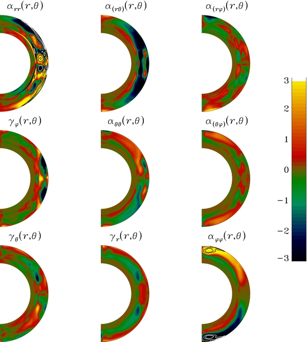
Figure 9. Components of the α-tensor, plotted in meridional plane. The color scale encodes the magnitude, in m s−1, and is the same for all plots. The three plots along the diagonal correspond to αrr, αθθ, and αϕϕ; the three plots above the diagonal to the corresponding off-diagonal component of the symmetric part of the tensor, and the three plots below the diagonal to the three components of the turbulent pumping velocity, as labeled and directly related to the three non-zero component of the antisymmetric part of the full α-tensor via Equation (25). The fitting procedure treats each hemisphere separately, so that the high degree of symmetry or antisymmetry about the equatorial plane characterizing the various tensor components is not a fitting artifact. A few isocontours are added to the two tensor components highly saturated by the adopted color scale: ±5, 10 m s−1 for αrr, and ±4, 5 m s−1 for αϕϕ.
Download figure:
Standard image High-resolution imageAlthough all components of the α-tensor are roughly of the same order of magnitude, the strongest components are found to be αrr and αϕϕ, both antisymmetric about the equatorial plane. The former is highly structured spatially, peaking in subsurface layers and in the equatorial regions and with numerous sign changes in each hemisphere. The latter is spatially more homogeneous, with sign changes only across the equatorial plane and across a near-spherical surface located above the core–envelope interface, at r/R ≃ 0.76. Significant amplitudes are obtained in the off-diagonal contributions, particularly α(rθ) and its associated pumping velocity γϕ. This can be traced to the development of persistent non-axisymmetric flow structures in the low-latitude portions of the outer convection zone (see Figure 4), which contribute a strong signal to the "small-scale" flow component even after the azimuthally averaged mean-flow is subtracted (viz., Equation (11)). These flow structures are also responsible for the strong low-latitude signal seen in αrr.
The αϕϕ component is of particular interest here, as it is the primary contributor to the production of the large-scale poloidal magnetic component (cf. bottom panel on Figure 2). Its first important structural property is antisymmetry with respect to the equatorial plane, as expected for cyclonic turbulence, where reflectional symmetry is broken by Coriolis forces (Parker 1955). Note that the fitting method we use to measure the components of the α-tensor treats each hemisphere independently, so that the high degree of antisymmetry observed here is a real characteristic of the simulation, rather than a fitting artifact. In the northern hemisphere, the αϕϕ component is positive in the bulk of the convection zone and peaks at high latitudes, as expected in view of the sense of twist imparted by Coriolis forces on diverging convective updrafts and converging downdrafts (Parker 1955). The sign change near the base of the convecting layer has been observed before in measurements of the α-tensor in other MHD simulations of convection (e.g., Ossendrijver et al. 2001) and is associated with the rapid decrease of the turbulent intensity as one moves downward toward and into the convectively stable fluid layer underlying the convection zone.
The SVD method has the additional advantage to automatically provide the variance in the estimate of a given parameter ak. Denoting this variance by σ2k, it is given by
The standard deviation (square root of variance) is in the range of 1–2 m s−1 in most of the convective layers for all α-components, but reaches much larger values in the underlying stable layers. This is inconsequential, as it arises simply because the EMF and large-scale magnetic field are both very weak below the convective zone, reducing greatly the quality of the fit in that region.5 Examination of the standard deviation distribution in meridional slices indicates that even though the stronger α-tensor components peak at high (αϕϕ) or low (αrr) latitudes, the absolute quality of the fit is actually best at mid latitudes, where the EMF signal is strongest (see Figure 8), as expected. Nonetheless, at mid-convection zone depth the inferred values of αϕϕ in polar regions deviate from zero by more than three standard deviations, leaving no doubt that these values are physically meaningful. On the other hand, in the equatorial region delimited by |θ| ≲ 30° and 0.7 ≲ r/R☉ ≲ 0.8 the standard deviation is of the same order of magnitude as αϕϕ, indicating a poorer fit in that area. This is simply due to the fact that both the EMF and the toroidal large-scale field are small in that region, as can be seen in Figures 2 and 8.
While the variance of the fit provided by the SVD is a useful, well-defined tool to characterize the accuracy of the fit, other methods can provide complementary information regarding the parameterization of the EMF. Here we demonstrate the quality of the fit by looking at the ability of the α-effect parameterization to reproduce the observed EMF from the α-tensor and the large-scale magnetic field. In Figure 10(A), we plot a time–latitude diagram of the residual between the observed EMF and the reconstructed EMF, i.e., the quantity

computed at depth r/R☉ = 0.85. It is quite remarkable to see that essentially no cyclic features remain in Δϕ. Apart from the equatorial band where the EMF barely manifests itself, there are in fact no clearly discernible structures in Δϕ. This implies that the α-effect parameterization performs very well at capturing the origin of the cyclic features of the EMF, the remainder of the EMF being essentially turbulent noise. This visual impression is confirmed by averaging latitudinally and performing a Fourier transform of the resulting time series to produce the power spectrum plotted in Figure 10(B). The low wavenumber portion of this spectrum is tolerably well represented by a 1/f power law and does not show any particular features or changes in slope at frequencies corresponding to the cycle period of the large-scale field or its first few harmonics.
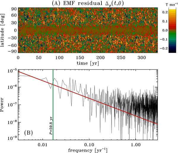
Figure 10. (A) Time–latitude diagram of the EMF residual defined by Equation (34), constructed on a sphere of radius r/R☉ = 0.85. (B) Power spectrum of the residuals of part (A) averaged in latitude to produce a simple time series. The sloping red line is a guide to the eye, showing a 1/f spectrum. The vertical line segment indicates the frequency corresponding to the primary magnetic cycle (full period 59.8 years).
Download figure:
Standard image High-resolution image3.5. Turbulent Pumping
The three meridional slices under the diagonal in Figure 9 represent the components of the turbulent pumping speed, as defined through Equation (25). The vertical component γr is found to be negative through most of the convective envelope, with upward pumping taking place only in the subsurface layers. This is better viewed in Figure 11 showing radial cuts of γr extracted at latitude +45° (panel A, solid line) and latitudinal cuts extracted at depth r/R☉ = 0.75 (panel B). This is qualitatively similar to the results obtained by Ossendrijver et al. (2002, see their Figure 5) in their local Cartesian simulations including rotation.6 This downward pumping reaches significant speeds, ∼1 m s−1 in the bottom half of the convective layers, except at very low latitudes where it all but vanishes. Upward pumping occurs at all latitudes for r/R☉ ⩾ 0.9, except at very low latitudes |θ| ⩽ 15°), where the γr > 0 region reaches almost to the base of the convecting layer (see Figure 9, central bottom meridional slice).
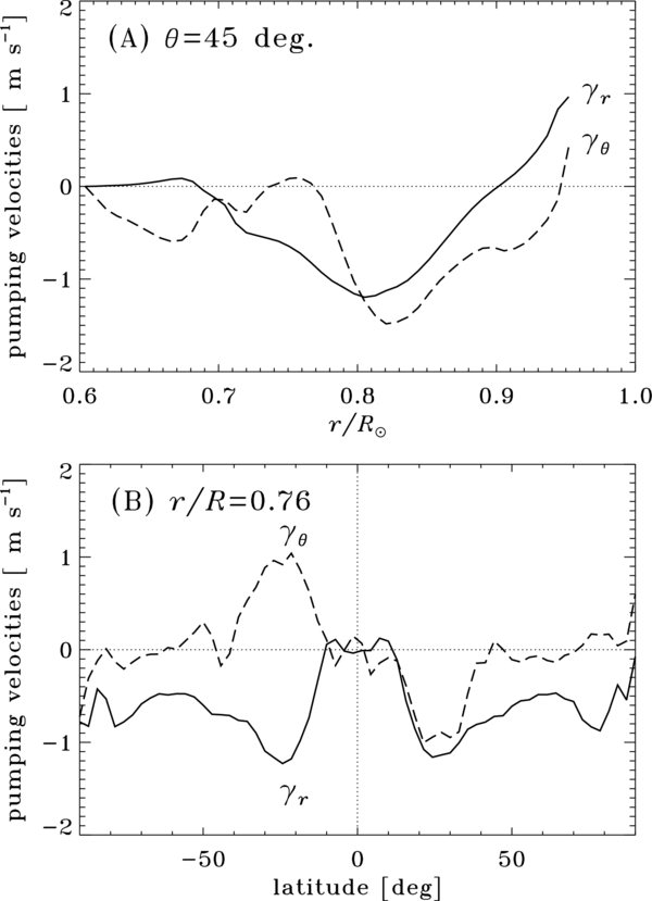
Figure 11. (A) Radial and (B) latitudinal cuts of the radial (solid lines) and latitudinal (dashed lines) turbulent pumping velocity components, extracted at latitude 45° in (A), and at depth r/R☉ = 0.76 in (B). Radial pumping is downward in the bulk of the convecting layers, except near the surface, while latitudinal pumping is equatorward at mid to low latitudes. See also the bottom-left (γθ) and bottom-middle (γr) panels in Figure 9.
Download figure:
Standard image High-resolution imageWe also detect in our simulation a significant equatorward latitudinal pumping in the outer two thirds of the convective envelope (see the bottom-left meridional slice in Figure 9 and dashed lines in Figures 11(A) and (B)), particularly prominent at mid latitudes where it reaches ∼1 m s−1 in the middle of the convection zone. Both the direction and magnitude of this latitudinal pumping velocity are similar to those measured in the local simulations of Ossendrijver et al. (2002). Again, like these authors, we also observe significant poleward latitudinal pumping in the subsurface layers of the simulations, with speeds approaching 2 m s−1 at latitude |θ| ≃ 60°. Given the ∼30 year duration of our cycles, it is therefore quite possible that the poleward drift and intensification of the surface magnetic field seen on the bottom panel of Figure 2 is driven at least in part by turbulent pumping, as proposed already by Ossendrijver et al. (2002).
It is also interesting to compare the turbulent pumping velocity to the drift speed of the large-scale toroidal magnetic field visible on the top and middle panels of Figure 2. The net drift speed of large-scale magnetic structures is influenced by other physical processes, notably turbulent diffusion. Indeed, if turbulent pumping plays a role in this drift its speed should still have values of the same overall order of magnitude as to the observed drift speeds. For most cycles, the equatorial drift of the toroidal component at the core–envelope interface (Figure 2, top panel), as measured by tracking the latitude of peak mean toroidal magnetic field at any given time, spans 25°–30° in 20–25 years, depending on individual cycles. This yields drift speeds in the range 0.3–0.5 m s−1. Both the magnitude and direction of this drift compare well to the mid-latitude latitudinal turbulent pumping speed |γθ| ≃ 0.2 m s−1 at r/R☉ = 0.718, as plotted in Figure 11(A). Likewise, measuring the slope from r/R☉ = 0.8 to 0.7 of the polarity reversal line on the middle panel of Figure 2 leads to a radial drift speed ∼−0.1 m s−1, only a factor of five smaller than the mid-latitude values of γr in this range of depth, as plotted in Figure 11(A). All of this suggests that turbulent pumping may well play an important role in the spatiotemporal evolution of the large-scale, mean magnetic field building up in the simulation.
3.6. α-quenching and Cycle Amplitude Saturation
We next turn our attention to the possible time dependence of the tensor αij. Our entire analysis so far relies on the assumption that αij depends only on position and not time. As we have just shown, this hypothesis works fairly well in practice, in the sense that it provides an accurate parameterization of the EMF in terms of the large-scale magnetic field. At a more physical level, there are however reasons to believe that the α-effect could vary in time via a nonlinear dependence on the magnetic field strength.
In the solar context, the α-effect can arise via the systematic twist imparted by cyclonic convection on a pre-existing large-scale magnetic field. This idea was introduced by Parker (1955), who argued that it could circumvent Cowling's theorem by providing a viable regeneration mechanism for the Sun's large-scale poloidal magnetic component. Because magnetic tension should resist any twisting by the flow, it has been argued that Parker's mechanism can only operate up to the point where the large-scale magnetic field reaches local equipartition with the turbulent fluid motions. This has led to the introduction of a number of simple so-called α-quenching algebraic formulae, e.g.,
where Beq is the equipartition magnetic field strength (see also Rüdiger & Kitchatinov 1993).
In order to explore if the α-effect varies from one cycle to the next, in a manner related to the strength of the mean magnetic field, we refine our analysis by breaking up the simulation data into blocks each spanning 100 solar days (∼8 years). One set of blocks is centered on times of cycle maximum, when the large-scale magnetic field reaches peak strength, and a second set of interweaved blocks is centered on times of polarity reversals, where the large-scale magnetic component reaches its minimum. Because of the regularity of the cycles in the simulations (see Figure 2), and good hemispheric synchrony, such a partition of the simulation can be unambiguously defined and readily carried out. We then apply the fitting procedure described previously to each block of data independently, which yields a sequence of functions {αij(r, θ, tc)}, where tc is the time around which a given block is centered.
With the SVD fit now carried out over a much reduced time span, the resulting α-tensor is much noisier, with the standard deviation associated with the fit now often exceeding the fitted values themselves. In order to extract a statistically meaningful signal from these results, we spatially average the α-tensor components over meridional planes for each tc, yielding a single measure αc for each time block; for example, applying this procedure to the αϕϕ component

Note that we use the standard deviation returned by the SVD algorithm as a weighting factor on the values being averaged. The radial integration bounds rmin and rmax are chosen to include the convective zone, but not the stable layers (r/R☉ ⩽ 0.718) nor the surface of the simulation, in order to capture the contributions from regions where the α-effect is expected to operate substantially. The latitudinal integration is restricted to either the north or south hemisphere, to avoid uninteresting cancellations as the sign of αϕϕ flips from one hemisphere to the other. The standard deviation on the spatially averaged quantity is computed as

where A is the surface over which the above averaging integrals are defined. This amounts to treating the integral as a weighted sum of statistically independent measurements, probably a debatable hypothesis here, but nonetheless sufficient for the foregoing analysis.
The results of those calculations, as applied to the αϕϕ component, are shown in Figure 12, where each histogram-type column represents one temporal block. The total width of the error bars is given by 2σc. Viewed in this way, the actual values of αc do not vary substantially in both hemispheres throughout the entire simulation and do not appear to show any clear, systematic variations between maximum and minimum phases. Similar results are obtained for the other components of the α-tensor. The αϕϕ component does show a very weak (r = −0.27) anticorrelation with the mean magnetic field strength spatially averaged in each time block, but even there the range of variation is only about one-half of the standard deviation.
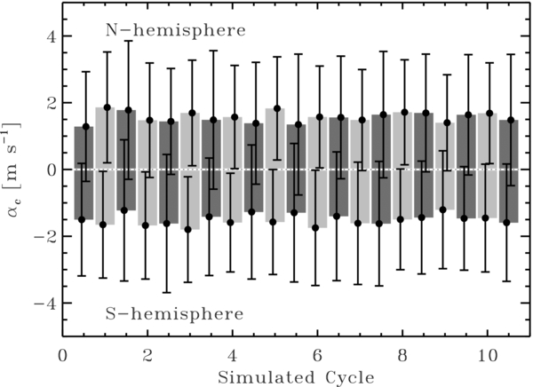
Figure 12. Temporal variation of the spatially averaged αϕϕ tensor component, computed separately in each hemisphere according to Equation (36b); this yields positive (negative) values in the northern (southern) solar hemisphere. The darker shading corresponds to blocks centered on times of maxima in  , and the lighter shades to interleaved blocks centered on times of polarity reversals. The error bars are computed from the variance returned by the SVD fitting algorithm via Equation (33). Qualitatively similar results are obtained for other α-tensor components, i.e., no systematic, statistically significant variation between epochs of cycle maxima and minima.
Download figure:
Standard image High-resolution imageIn an attempt to further suppress the noise, we then used the SVD fitting algorithm to do a single fit on all time blocks associated with maximum phases, and a separate fit for all time blocks centered on minimum phases. The resulting α-tensor components were then averaged spatially in the same manner as previously. The resulting αc values, again for the ϕϕ component, are listed in Table 1 with the corresponding spatial average for the αϕϕ component extracted from the full simulation run, as plotted in Figure 9 (bottom right). Here we finally obtain a min/max difference that exceeds the range of the estimated error bars, and which moreover runs in the direction expected from the idea of α-quenching, namely a weaker αc when the mean field is strongest. However, the associated variation in αc between maximum and minimum phases remains rather modest, at the 20% level for the southern hemisphere, down to the 10% level in the northern.
Table 1. Hemispherically Averaged αϕϕ (m s−1)
| Epoch | Northern Hemisphere | Southern Hemisphere |
|---|---|---|
| Maxima | +1.682 ± 0.069 | −1.571 ± 0.067 |
| Minima | +1.871 ± 0.059 | −1.919 ± 0.070 |
| Full run | +1.712 ± 0.011 | −1.750 ± 0.011 |
Download table as: ASCIITypeset image
The results of Table 1 reflect the variation of the spatially integrated α-profiles and could of course hide more substantial local variations. This is examined in Figure 13, showing now the spatial distribution of the αϕϕ component extracted from the set of concatenated data blocks centered on cycle minima (top row) and maxima (bottom) row, together with the corresponding spatial distributions of the standard deviation returned by our SVD fitting scheme (at right). At first glance both distributions appear quite similar, but a closer look reveals a marked reduction of αϕϕ at the base of the convection zone at maximum epochs, as well as at high latitudes. While these amplitudes of these variations (by ∼1–2 m s−1) are well within the local one standard deviation at high latitude (∼2–4 m s−1), at lower latitude they are comparable or slightly larger than one standard deviation, suggesting a statistically significant local variation. Note also that this is also where the toroidal large-scale component reaches its peak value (see Figure 2), so this is in fact where α-quenching would be expected to be most important.
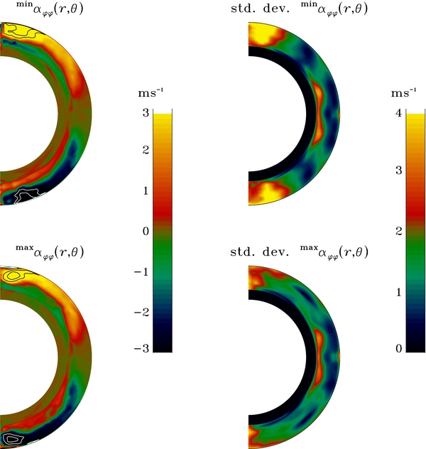
Figure 13. αϕϕ tensor component extracted from two concatenated sets of disjointed data blocks, the first centered on epochs of cycle minima (top left), the other on cycle maxima (bottom left). The color scale is the same as in Figure 9, with additional contours overlaid for values ±4 and ±6 m s−1. The two meridional plane diagrams on the right show the corresponding standard deviation returned by the SVD fitting algorithm. Compare the left plots to the bottom-right plot in Figure 9, showing the same component fitted over the full simulation span. While the min/max differences are largest at high latitudes, they only exceed the standard deviation at mid latitudes near the base of the convective envelope, where the large-scale toroidal field is strongest (cf. Figure 2).
Download figure:
Standard image High-resolution imageIn contrast to the αϕϕ component, αrr, αθθ as well as the radial pumping velocity γr shows no significant local variation whatsoever between maximum and minimum epochs. Other components show high-latitude variations, but all at or within the associated one standard deviation range. In fact, the only other noteworthy pattern is a significant enhancement of the poleward latitudinal turbulent pumping in the surface layers at maximum epochs, by a factor of nearly two, which is slightly larger than the local one standard deviation range for γθ.
Taken as a whole, the results presented above indicate that little or no significant α-quenching occurs in our simulation, i.e., the magnitude of the α-tensor components is for the most part insensitive to the value of the large-scale magnetic field. This justifies, a posteriori, our use of the tensorial expansion of the turbulent EMF in terms of the mean magnetic field (viz., Equation (22)), as the starting point of the analysis carried out throughout this section.
4. RELATIONSHIP TO MEAN-FIELD DYNAMO MODELS
The scale separation and azimuthal averaging introduced earlier jointly form the basis of the so-called mean-field dynamo models, which have been and continue to be used extensively in studying solar and stellar magnetic activity cycles. If one assumes at the onset that the large-scale magnetic field  is axisymmetric, then it can be expressed as the sum of a toroidal component and poloidal component defined through a purely azimuthal axisymmetric vector potential
  , as
, as

One can further assume that the mean flow is also axisymmetric and comprised only of differential rotation, i.e.,

where ϖ ≡ rcos θ and Ω is the (axisymmetric) angular velocity. Under those assumptions, Equation (20) for the mean field is then readily separated as
for constant η and under the Coulomb gauge  .
.
Equations (40)–(41) are known as the mean-field dynamo equations, and models based on these equations (or variations thereof) remain to this day the workhorse of solar cycle modeling, interpretation, and even prediction (see, e.g., Charbonneau 2010 and references therein). They show the critical importance of the mean EMF in such axisymmetric mean-field models; the EMF provides a source term on the right-hand side of the evolution equation for 〈Aϕ〉, without which dynamo action is impossible, as per Cowling's theorem. It also provides a source term for the toroidal component 〈Bϕ〉, but here it is less crucial because differential rotation already provides a source contribution, provided a poloidal magnetic component is present. The so-called αΩ dynamo model results from dropping the α-effect term in Equation (41), while dropping instead the differential rotation shearing term yields the α2 model, in which the turbulent EMF is the sole inductive mechanism. Retaining all terms leads to the α2Ω mean-field dynamo model.
4.1. Contributions to Toroidal Field Induction
To which (if any) of these three possible mean-field model categories could we identify our simulation? The answer clearly hinges on the relative importance of the  and
and  terms on the right-hand side of the mean-field induction Equation (20). In keeping with our "experimental" approach, we simply use the mean and fluctuating flow and magnetic field components defined previously do directly calculate, using simple centered finite differences, the azimuthal components of both
  and
and  , which then measures the rate of change of the magnetic field associated with each inductive contribution.
Figure 14 shows the results of this exercise, in the form of time–latitude diagrams for the azimuthal component of each of these two contributions (top and middle rows), as well as their sum (bottom row), extracted at the base of the convection zone (r/R☉ = 0.718, left column) and higher up in the convection zone (r/R☉ = 0.803, right column). The time span covered corresponds to the second half of the simulation run. It must be remembered that computed in this manner, the plotted tendencies reflect not only the action of source terms but also transport by turbulent pumping and large-scale flows.

Figure 14. Time–latitude diagrams for the azimuthal components of the inductive contributions  (top panel) and
  (middle panel), constructed at depth r/R☉ = 0.718, at the base of the convection zone (left column) and at r/R☉ = 0.803 (right column). Both contributions are here roughly of the same order of magnitude but have opposite signs at most latitudes. The sum of the top and middle panels is shown on the bottom panels, using the same color scale and ranges; this gives the expected rate of change of the mean azimuthal field, itself overlaid as black (white) contours for 〈Bϕ〉 > 0 (<0).
Download figure:
Standard image High-resolution imageAt any phase of the cycle, both contributions are here clearly of the same overall order of magnitude. Furthermore, constructing similar diagrams at other depths indicates that this remains the case throughout the bulk of the convection zone. In the terminology of mean-field electrodynamics, one would then conclude that in this one specific simulation, the large-scale magnetic field is sustained by an α2Ω dynamo, in the sense that both source terms on the right-hand side of Equation (41) contribute to the evolution of the toroidal field. However, it is also clear from Figure 14 that these two contributions to toroidal field production act in opposition to each other at most latitudes during most phases of the cycle. Interestingly, a similar pattern was observed in the MHD simulations of Brown et al. (2010), which produced steady large-scale magnetic fields. In their simulations D3 (see their Section 5.1), production of toroidal magnetic fields by the large-scale differential rotation shear was found to dominate over an opposing turbulent induction and Ohmic dissipation. Here, in the absence of explicit Ohmic dissipation and with both contributions to toroidal field production of comparable strengths, sign notwithstanding, the net tendency (bottom row) shows a spatiotemporal evolution that is markedly different from either contribution, and overall much smaller in magnitude.
The solid contours in Figures 14(C) and (F) show the spatiotemporal evolution of the large-scale toroidal magnetic component at the corresponding depths. At the base of the envelope the 〈Bϕ〉 component and its temporal variation reconstructed from the upper two panels, shown as color levels, are seen to be offset in time, with d〈Bϕ〉/dt leading 〈Bϕ〉 in a manner consistent with the development of the observed polarity reversals at that depth. This phase offset, in turn, results from the residual tendency left from the near cancellation of the turbulent EMF and large-scale shear contributions plotted in panels A, B, and D, E. A similar temporal offset is observed at mid-convection zone depth at the mid latitudes, but not in the vicinity of the equatorial plane.
These results, especially when considered jointly with those of Brown et al. (2010, 2011), suggest that the development of cycles arises through a rather delicate balance between the magnitude and relative phasing of turbulent induction and large-scale shear. One could then legitimately suspect that the cycle period in these simulations is also sensitively dependent on this balance, which is itself likely dependent on various simulation parameters such as rotation rate, forcing, stratification, and so on. How and when the transition from steady to cyclic dynamo action takes place requires a detailed parameter study, which goes well beyond the scope of the present paper. Nonetheless, the demonstrated difficulty in "finding" regular cyclic large-scale dynamo action in these kinds of turbulent simulations, at the solar rotation rate at least, may well be a reflection of the need for such a fine balance to materialize.
4.2. Relating the α-tensor to Kinetic and Magnetic Helicities
The mathematical machinery of mean-field electrodynamics also involves the characterization of the turbulent EMF in terms of the mean magnetic field. In particular, for turbulent flows satisfying certain statistical properties and operating in certain specific physical regimes, it offers the mean of calculating the form of the α-tensor (see, e.g., Moffatt 1978). In the case of a turbulent flow that is isotropic and homogeneous but lacks reflectional symmetry, the α-tensor reduces to the diagonal form αδjk, with
where τ is the correlation time of the turbulence and hv is the mean kinetic helicity associated with this turbulent flow:

The key result here is that albeit for the sign difference, the α-effect coefficient is directly proportional to the kinetic helicity, a quantity readily computed a posteriori from the simulation output. The result of such a calculation is plotted in Figure 15(C), with the kinetic helicity having been averaged temporally as well as azimuthally over the complete time span of the simulation. Except for the sign difference, the degree of resemblance with the αϕϕ tensor component plotted on panel A is quite striking. Both functionals are strongly peaked at very high latitudes, and in each hemisphere only show a sign change near the base of the convection zone. The most prominent difference is found at low latitudes, where hv shows a secondary peak in the middle of the convection zone that is absent in the αϕϕ profile. The αθθ component (see Figure 9) is also tolerably well represented by the negative of the mean kinetic helicity, the most prominent discrepancy being that αθθ peaks at mid latitudes. The αrr diagonal component is that which shows the least similarity with the mean kinetic helicity, presumably because it is more sensitive to the break of homogeneity on which Equation (42) is predicated, induced by stratification of the background state and/or upper boundary condition. Another significant departure relates to the temporal behavior of the kinetic helicity, which shows a clear signature of the cycle in the large-scale magnetic field, while most α-tensor components extracted from the simulation do not, at least not at a level that could be deemed statistically significant; in the simulation, the cyclicity of the EMF is well captured by the cyclicity of the large-scale magnetic component (viz., Figure 10).
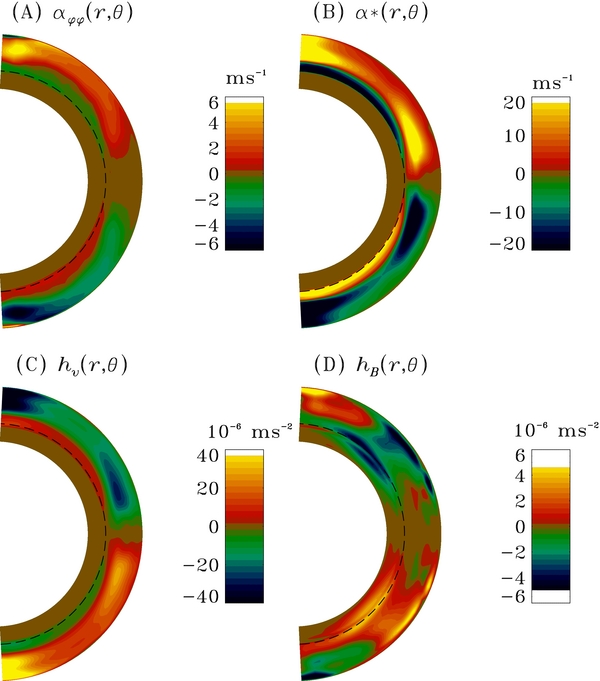
Figure 15. Meridional slice plots of (A) αϕϕ, replotted directly from Figure 9; (B) is the corresponding tensor component reconstructed from Equation (44), using the temporally and zonally averaged kinetic and magnetic helicity profiles extracted from the simulation and plotted on panels (C) and (D), respectively. The correlation time τ is computed according to Equation (46) and is set to zero below the core–envelope interface r/R = 0.718, indicated by the dashed circular arc on all panels.
Download figure:
Standard image High-resolution imageEquation (42) is also predicated on a number of other strong assumptions, including the requirement that the small-scale turbulent flow remains entirely unaffected by the small-scale turbulent magnetic field. Once the latter becomes dynamically significant, it is expected that it will alter the small-scale flow giving rise to the α-effect. Based on a set of local Cartesian incompressible MHD simulations operating in the strongly nonlinear regime, Pouquet et al. (1976) suggested that Equation (43) should be replaced by
where hB is the mean current helicity, generalized to our anelastic MHD formulation as

The physical link between kinetic and current helicity becomes more transparent upon noting that  is the Alfvén velocity, measuring the propagation speed of transverse MHD waves for which magnetic tension provides the restoring force; in essence, what Equation (44) expresses is simply that magnetic tension tends to oppose any twisting of magnetic field lines by the small-scale turbulent flow. The mean current helicity in our simulation is plotted in Figure 15(D), again as a combined azimuthal and temporal average spanning the full simulation duration. This magnetic contribution to the α-coefficient is found to be significantly smaller than its kinetic counterpart, by a factor of about 10. The strong peaks straddling the base of the convection zone at mid latitude in both hemispheres are associated with the strong mean magnetic field building up in these regions, which, acted upon by the small-scale turbulent flow, feeds the production of small-scale current helicity.
Figure 15(B) shows the α*(r, θ) profile reconstructed according to Equation (44). The correlation time within the unstable layers is estimated in a similar manner as in Brown et al. (2010), i.e.,
where Hρ is the density scale height of the background stratification and u' is the rms average of the small-scale flow component, the averaging being carried out zonally, latitudinally, and temporally over the full time span of the simulation. In the stable layers, τ is artificially set to zero, since Equation (44) is not expected to hold there, pertaining as it does to fully developed turbulence.
With the kinetic helicity about an order of magnitude larger than the magnetic helicity, the structure of this estimated α*(r, θ) reflects primarily the spatial structure of the kinetic helicity, except in the immediate vicinity of the core–envelope interface where the kinetic and magnetic contributions have comparable magnitudes. While the overall amplitude of this reconstructed α profile is about a factor of three larger than the measured αϕϕ (Figure 15(A)), in terms of the spatial variations Figures 15(A) and (B) are remarkably similar. Interestingly, the overall magnitude of the reconstructed α, ∼20 m s−1, is quite comparable to the α reconstructed similarly in Brown et al. (2010, see their Figure 8) in a simulation rotating at thrice the solar rate, and sustaining a temporally steady, rather than cyclic, large-scale magnetic field component.
The limited applicability of Equation (44) to our simulation notwithstanding, the weak contribution of the specific current helicity as compared to the kinetic helicity term suggests that the dynamical impact of the small-scale magnetic component on the small-scale flow is correspondingly weak. Recall that we also demonstrated, in Section 3.6, that the α-tensor components show little or no significant variation with the strength of the large-scale magnetic field. This would suggest that the α-effect in our simulation operates in the quasi-linear regime and that the saturation of the dynamo amplitude must be achieved via a different mechanism.
5. DISCUSSION AND CONCLUSION
We have investigated the mode of large-scale dynamo action taking place in the global implicit large-eddy simulation of the solar convection zone reported in Ghizaru et al. (2010). Motivated by the presence of a strong and well-defined axisymmetric magnetic component arising in the simulation, we defined the large-scale magnetic field as the longitudinal average of the total simulated magnetic field, with the residual produced by subtracting this average component from the total field defining the small-scale, fluctuating magnetic component. Zonally averaging the cross-correlation of the latter with the corresponding small-scale flow component then permits the calculation of a turbulent EMF, and its development in terms of the large-scale, zonally averaged component allows us to calculate the components of the α-tensor. The α-tensor components so calculated were found to compare well to a number of results obtained in local Cartesian simulations with an externally imposed large-scale magnetic component. Noteworthy results include a positive αϕϕ component in the northern solar hemisphere, peaking at high latitude and changing sign near the base of the convecting shell; downward turbulent pumping in the bulk of the convection zone, except in a thin subsurface layer where pumping is upward-directed; and significant latitudinal pumping, equatorward at mid to low latitude in the bulk of the convecting layer, but poleward in the high latitude, subsurface layers.
Because our simulation generates its own large-scale magnetic field, no such field need be imposed externally to measure the α-effect. The α-effect that we do measure is then dynamically consistent with the nonlinear interaction of flow and field at all numerically resolved spatial and temporal scales. However, our analysis is physically meaningful only to the degree that the scale separation procedure used to divide the total flow and field into mean and fluctuating components is applicable to our simulation results. The modal analysis described in Section 3.1 suggests that it is. Moreover, Figure 10 provides additional empirical evidence that something closely akin to the α-effect of mean-field electrodynamics offers an adequate representation of the turbulent EMF arising in the simulation.
The mean-field analysis reported upon in this paper relies entirely on a posteriori calculations of cross-correlations between the small-scale flow and magnetic field, as defined via Equations (11) and (12) and as resolved by our computational grid. The implicit presence of dissipative terms at the truncation level of the MPDATA advection scheme at the core of EULAG has been shown, in the context of purely hydrodynamical simulations, to mimic subgrid dynamical processes such as self-similar energy cascade (Domaradzki et al. 2003; Margolin et al. 2006; Margolin & Rider 2007). Evidently, the smallest resolved scales in our simulation have been influenced by these subgrid effects, and therefore so has our reconstructed EMF; however, the overall dynamo picture emerging from our analysis shows remarkable internal self-consistency, which suggests that MHD subgrid effects, if present, are not the primary direct drivers of cyclic evolution on large spatial scales.
The simultaneous presence of a globally well-structured α-effect and significant internal differential rotation suggests that our simulation could be operating as what is known in mean-field electrodynamics as an αΩ dynamo. This inference is buttressed by a number of simulation features, notably the fact that the in-phase (or nearly so) production of a positive large-scale dipole moment from a positive toroidal component is what is expected of kinematic αΩ dynamo models having the angular velocity outwardly increasing and αϕϕ > 0 in the northern solar hemisphere (see Stix 1976). Oscillatory behavior has been shown to be possible also in linear α2-type models, i.e., in the complete absence of differential rotation, provided the α-effect has sufficiently steep radial variations, including sign changes (Stefani & Gerberth 2003). Such oscillatory α2-type solutions were recently identified in the helically forced MHD simulations of Mitra et al. (2010). These authors also presented specific examples showing that such externally forced α2 dynamo models could also exhibit latitudinal propagation of the azimuthal large-scale magnetic component. Given the rather complex spatial variations of our measured α-tensor components (see Figure 9), it then remains possible that the α-effect is the primary driver of the polarity reversals and mild equatorward propagation of the deep-seated mean magnetic component observed in our simulation. Then again, the comparable magnitudes of the small-scale and large-scale contributions to the ϕ-component of the induction term (cf. Figures 14(A) and (B)) would rather point to the so-called α2Ω dynamo, in which shearing by the large-scale flow and the turbulent EMF both contribute to the regeneration of the large-scale toroidal magnetic component. Unless differential rotation is very weak, such dynamos behave qualitatively like αΩ dynamos. In particular, they also support traveling dynamo waves propagating according to the Parker–Yoshimura sign rule (see, e.g., Choudhuri 1990; Charbonneau & MacGregor 2001). At a given turbulent intensity, the distinction between these three classes of models therefore hinges on the magnitude of differential rotation in the region where dynamo action is taking place.
Interestingly, the pole-to-equator angular velocity contrast in a purely hydrodynamical simulation using the same stratification and thermal forcing as in Ghizaru et al. (2010) is much closer to solar (cf. Figures 3 and 4), indicating that the magnetic field—both small scale and large scale—has a significant impact on the dynamics of large-scale flow building up in the simulation. A similar behavior was observed already in the simulations of Gilman (1983) and carried over also to the more strongly turbulent simulations of Browning et al. (2006). Assume for the sake of the discussion that a stronger, solar-like internal differential rotation could be produced in our simulation, e.g., by introducing a latitudinal gradient in the thermal forcing, as done in Miesch et al. (2006) and Browning et al. (2006). In kinematic αΩ mean-field models operating close to criticality, the cycle frequency is found to increase as a power, usually close to unity, of the so-called dynamo number D, defined as
where R is a measure of the size of the dynamo region (often taken as the solar/stellar radius), α0 measures the magnitude of the α-effect, ΔΩ that of the differential rotation, and ηT is the turbulent diffusivity value used in the model. Consider now our simulation; assuming that ramping up ΔΩ by a factor of three can be achieved without affecting the EMF or (implicit) turbulent diffusivity too much, Equation (47) would then predict a decrease of the cycle period by a factor of ∼3, which would bring it down to the solar value. This would alleviate simultaneously two of the primary failings of the present simulation as compared to the solar cycle, namely the latitudinal surface differential rotation being too weak and the cycle period being too long. On the other hand, the fact that the large-scale surface poloidal and deep-seated toroidal components oscillate almost exactly in phase may well lie outside the reach of these types of global MHD simulations. Modeling of the solar surface magnetic flux evolution (e.g., Wang & Sheeley 1991; Schrijver et al. 2002; Baumann et al. 2004) has shown that the poleward transport of magnetic decay products of sunspots and active regions by supergranular diffusion and the poleward meridional flow is an important driver of polar field reversals. There is of course nothing equivalent to decaying active regions in our simulations, so in retrospect an incorrect timing of surface polar field reversals is perhaps not exceedingly worrisome.
The question of cycle amplitude saturation also merits further investigation. The analysis of Section 3.6 suggests that if something like classical α-quenching by the mean magnetic field is taking place, it is at a rather modest level, globally of the order of ∼10%–20%. Unless the dynamo is only very mildly supercritical, this is likely insufficient to provoke amplitude saturation. In addition, the analysis of Section 4.2 suggests that quenching by the small-scale magnetic component is also insignificant, current helicity being almost an order of magnitude smaller than kinetic helicity in the bulk of the convecting layers. Moreover, and even though it is defined globally, the steadiness of the E(u') time series plotted in Figure 5 is consistent with the conclusion drawn on the basis of Figure 12, namely that the α-tensor is not affected significantly by the presence of the large-scale magnetic field. On the other hand, the energy contribution associated with the large-scale flow does show a fairly clear cyclic variation, approximately in anti-phase with the large-scale magnetic energy for most cycles; and, as we noted already, the latitudinal differential rotation is much weaker in the MHD simulation than in its purely hydrodynamical counterpart. This suggests that dynamo saturation takes place via magnetic backreaction on the large-scale flow. It remains to be investigated whether this backreaction is mediated by the Lorentz force component associated with the large-scale magnetic field (the so-called Malkus–Proctor effect), or through small-scale Maxwell stresses, either directly or through quenching of the small-scale Reynolds stresses powering the large-scale flow (sometimes referred to as Λ-quenching; see, e.g., Kitchatinov & Rüdiger 1993; Rempel 2006, and references therein).
Another intriguing question relates to the mechanism(s) responsible for the equatorward propagation of the sunspot activity belts in the course of the cycle. If sunspots are assumed to originate from the destabilization and vertical rise of toroidal magnetic flux ropes stored immediately beneath the solar core–envelope interface, then the observed equatorward drift should reflect a similar drift in the deep-seated toroidal magnetic components from which these flux ropes are believed to form. The weak equatorial propagation visible on the top panel of Figure 2 amounts to a drift speed in the range of 0.3–0.5 m s−1, while in the Sun this speed is estimated at 1 m s−1. In the simulation considered here, a weak positive radial differential rotation is sustained at mid to low latitudes at the core–envelope interface. In conjunction with a negative αϕϕ at the base of the envelope (see Figure 9, bottom-right meridional slice), we then have αϕϕ × dΩ/dr < 0, which should then lead to an equatorward propagation of the dynamo wave as per the Parker–Yoshimura sign rule. Then again, our simulation is also characterized by a mean meridional flow component which, at mid latitude at the core–envelope interface, is equatorward and reaches a few tenths of meters per second, comparable to the drift speed inferred from Figure 2. Moreover, as discussed in Section 3.5 the latitudinal turbulent pumping at the base of the envelope is equatorward and also reaches a few tenths of meters per second. In our simulations, the large-scale differential rotation and meridional flow both show significant temporal variations in phase with the cycling large-scale magnetic field, and the energy density of the large-scale flows and field are commensurate (cf. Figure 5). Particularly in the case of the meridional flow, it is not clear a priori whether the observed cyclic variations locally drive, or are driven by, cyclic variations in the large-scale magnetic component. Clarifying this question again requires a complete and detailed investigation of the dynamical balance arising in the simulation. Such an analysis is now underway and will be reported upon in a forthcoming paper.
We wish to thank the referee for a very useful and constructive report. The numerical simulations reported upon in this paper were carried out primarily on the computing facilities of the Réseau Québécois de Calcul de Haute Performance. This work is supported by Canada's Natural Sciences and Engineering Research Council, Research Chair Program, and Foundation for Innovation (E.R., P.C., M.G., and A.B.), as well as by the Space Science Enhancement Program of the Canadian Space Agency (grant 9SCIGRA-21). P.K.S. acknowledges support by the DOE award DE-FG02-08ER64535. The National Center for Atmospheric Research is sponsored by the National Science Foundation.
Footnotes
- 4
Since the quantities considered in this section are constructed from azimuthal averages, our computational grid is reduced to two spatial dimensions here.
- 5
Essentially, where both the EMF and
 are weak, the fitting algorithm attempts to obtain αij by inverting a problem that is numerically ill-posed. Schematically, this amounts to solving α = δ/
 , with α of order unity, but with both δ and being very small.
 - 6
Note that although we both use right-handed coordinate systems, the pseudoradial z-direction in Ossendrijver et al. (2002) points into the domain, while our radial r-direction points outward; therefore, a positive γr does correspond to a radially upward flow component in our simulation, while a positive γz defines a downward flow in Ossendrijver et al. (2002). Our respective "latitudinal" unit vectors are however oriented in the same way, i.e., northward, so that our γθ is directly comparable to their γx.
