


ABSTRACT
In 1995, a binary black hole model was proposed for the quasar OJ287, where the smaller secondary black hole impacts the accretion disk of the primary black hole twice during its 12 yr orbit and causes a double peak of optical outbursts. The model predicted four major outbursts and one minor outburst during the period 1996–2010. All five have now been observed. In this paper, we ask how accurate the predictions were. We use the latest optical observations from Tuorla Observatory and the KVA telescope at La Palma together with previously published data to construct a light curve for this period. We average the data in 0.04 yr bins, and subtract the observed flux from the 1995 model flux at each bin. We find that the residuals are small: they are well described by random noise of amplitude 1.4 mJy. This level is small compared with the amplitudes of the major outbursts, 5–7 mJy. Ignoring the noise, the binary model explains the optical data remarkably well.
Export citation and abstract BibTeX RIS
1. INTRODUCTION
The quasar OJ287 has been observed to go into major outbursts at about 12 yr intervals since 1890s. The period is not exact: the outburst times deviate from the exact period by about a year either way (Sillanpää et al. 1988). After the 1994 predicted outburst had been observed (Sillanpää et al. 1996a), it became a challenge to see if there was any way of predicting the times of future outbursts more accurately. In general, there were two methods: one was to extrapolate from the past light curve. As Sillanpää et al. (1988) emphasized, this method could not give answers more accurately than by one year. For example, an outburst was predicted at 2006.3 ± 1 yr by this method.
A second method is to construct an astrophysical model. Sillanpää et al. (1988) suggested a binary model where a companion black hole in an elliptical orbit perturbs the accretion disk of the primary black hole during each pericenter passage, and causes increased accretion flow which eventually shows up as a brightening of the jet. Details of the process were not worked out, but it was suggested that this process would generate one broad outburst per period, with some of the secondary outbursts following suit.
This idea had two problems: the outbursts in OJ287 are often seen to be quite sharp, much sharper than the tidal timescale, and the outbursts are not periodic, unlike the tidal perturbations in a binary.
Thus, we need a model which is not periodic, and which can generate outbursts in a shorter timescale. Lehto & Valtonen (1996) realized that the binary model of Sillanpää et al. (1988) may be further developed by considering the impacts of the secondary on the accretion disk surrounding the primary. Since a relativistic binary black hole system must precess, a model of this kind naturally introduces some variation into the strict periodicity. The question was, does this explain the deviations from the exact periodicity? It turns out that with a proper choice of the eccentricity of the binary orbit and the precession rate of its major axis, the timings of the historical outbursts can be explained. In particular, the double peak structure in the light curve of OJ287 (Sillanpää et al. 1996b) gets a natural explanation, as every orbit must have two disk crossings. The two observed peaks are separated by 1–2 yr, which immediately gives the eccentricity of about 0.7. The modulation of the light curve with a period of 60 yr (Valtonen et al. 2006) gives the second parameter, i.e., the full precession cycle must be about 120 yr or 10 periods. Here and in the rest of this paper, the times are given in the observers' frame, which are a factor of 1.3 longer than the times in the frame of OJ287. Thus, the precession rate of the major axis must be around 36° per orbit. The more exact value is now known to be 39. 1 (Valtonen et al. 2010).
The combination of the disk impacts and the varying tidal transfer rate in the disk produces the full light curve. The calculations of this model were carried out in 1995 and were essentially completed in the summer of that year. The results were first described in 1996 February in the Miami meeting of the variability of blazars (Sundelius et al. 1996). The full results appeared in two papers (Lehto & Valtonen 1996; Sundelius et al. 1997); we call the model presented in these papers the 1995 model of OJ287.
In this paper, we first remind ourselves of the model and what it predicted for the future of OJ287. Then, we look at the optical monitoring of OJ287, which has been very intensive, perhaps more than with any other quasar, in the period 1996–2010. Then we conclude by discussing the agreement between the prediction and what actually happened.
2. THE 1995 MODEL
The 1995 model consists of three separate calculations. (1) Orbits are calculated in search of the optimal orbit parameters which produce the correct impact times on the accretion disk. This means thousands of trials and is extensive work in itself. The accretion disk is taken as a constant plane during this first step.
After the points of impact are known, one may proceed to step (2). There, one follows the evolution of a bubble of gas which is torn off the accretion disk at the impact. The bubble finally produces a sharp outburst when it becomes optically transparent. The quantities we need to know are the exact time of the outburst after the impact, called "time delay," and the size and the length of the outburst. Since the impact points vary, the evolution model has to be calculated individually for each impact. This is another major calculation. For this calculation the standard αg disk model of Sakimoto & Coroniti (1981) was used with reasonable parameter values. The disk is radiation pressure dominated in the region of interest. Such a disk is in accordance with the current understanding of accretion disks in quasars which are based on the family of α disks (Xie et al. 2009). The results of the first two steps were published in Lehto & Valtonen (1996).
Step (3) introduces the feedback on the disk. There are two major effects. First, the impact times are changed a bit when the disk does not stay in its original plane. As the disk is lifted toward the approaching secondary, the effect is to make the outburst happen sooner than in the fixed plane model. We call this advance the "time ahead," and it needs to be calculated for each impact separately. Second, the accretion flows induced by the secondary are calculated by following the flux of particles through a fixed radial distance. It does not matter much at what distance the measurement is carried out; for definiteness, the distance of 10 Schwarzschild radii of the primary was used as a standard. The disk was modeled by a 500,000 particle disk which means that very many trials could not be carried out in a reasonable amount of time. Details of two of the trials were published (Sundelius et al. 1996, 1997). The latter trial was carried out with two million particles.
The understanding of the 1995 model requires reading both papers (Lehto & Valtonen 1996; Sundelius et al. 1997). Also, one has to understand the limitations of a finite particle number simulation: the accretion flow per 0.04 yr bin consists of a relatively small number of particles. Thus, the Poisson noise makes a large contribution to the outward appearance of the predicted light curve. One should not confuse this with real predicted effects.
Two impact outbursts and three tidal outbursts were predicted for this period. One may take the tidal outburst predictions directly from the particle flux tracings (Sundelius et al. 1996, 1997), remembering the effect of the Poisson noise. The times of impact on the disk are also marked in these tracings. The related outbursts are a little delayed, but it is a simple matter to read off the delay, the size of the outburst, and the length of the impact outburst from Lehto & Valtonen (1996). For the 2005 outburst the delay is 0.49 yr, the size is 6.8 mJy, and the length of the outburst toutb is 0.129 yr. All of these values are either given directly or easily extrapolated from the tables. In Figure 1, the resulting light curve prediction is shown, and the five expected outbursts are numbered.

Figure 1. 1995 light curve of OJ287. Five major outbursts were predicted, with some enhanced activity in between, indicated by small peaks. The major tidal peaks (1), (4), and (5) are modeled by a simple fitting function applied to the tracing of Sundelius et al. (1996), while the impact peaks (2) and (3) follow the description of Lehto & Valtonen (1996).
Download figure:
Standard image High-resolution imageFor the tidal accretion flow, we have to consider what is physically significant and what is Poisson noise in the tracings of Sundelius et al. (1996, 1997). Here it is helpful to compare the tracings from the two independent runs. It shows that the significant information in the two tracings can be condensed in a simple light curve function of the form

where f is the increased accretion flux (number of particles crossing the 10 Schwarzschild radii circle per 0.04 yr time bin) and the time t is given in years. For the 1996 outburst we found the best fit with a = 7.4 and b = 0.5 yr, for the 2008 outburst a = 7.75 and b = 0.42 yr, while for the 2009 outburst a = 4.1 and b = 0.07 yr. Even though the 2009 outburst is smaller than the others, it appears similar in both tracings and thus is a real feature. The parameters are based on the model calculations alone, with no consideration of observed data.
Multiwavelength observations of OJ287 during outburst number (4) and their comparison with OJ287 in a quiet state show that the reason for brightening is most likely an increase in the number density of electrons (Seta et al. 2009). This is what we expect in the 1995 model where an increase in the accretion flow is thought to result in increased brightness. The model assumes a linear relationship between the increased optical brightness and the increased accretion flow. Preliminary tests of this idea imply that the actual relation is probably a power law rather than a direct proportionality (Valtonen et al. 2006). Such considerations were not part of the 1995 model and are not considered here.
However, the unpolarized nature of outburst number (3) favors the idea that the excess optical emission is dominated by bremsstrahlung (Valtonen et al. 2008), in accordance with the 1995 model. This is the signature of emission generated by the impact on the accretion disk.
3. OBSERVATIONS
We consider only a limited section of the light curve, from 1996 to 2010 January. The observations are taken from Valtonen et al. (2006), Wu et al. (2006), Valtonen et al. (2009), and Villforth et al. (2010) and the most recent data from the Tuorla and KVA observations. The magnitudes are transformed to the V band and converted to flux units. For details, see Valtonen et al. (2009).
The comparison with observations is carried out assuming that one unit in the particle flux corresponds to 2 mJy (Sundelius et al. 1996) or 0.5 mJy (Sundelius et al. 1997). This rule was found to apply prior to 1995 in explaining the earlier light curve.
Figure 2 displays the observations, averaged in 0.04 yr bins. Shorter timescale fluctuations may be significant but they are not part of the 1995 model, and thus are not discussed here. The 2007 September 13 outburst does not show well at this resolution. It has been described in detail elsewhere (Valtonen et al. 2008).

Figure 2. Observations of OJ287 during 1996–2010. The numbers labeling the outbursts are the same as in Figure 1.
Download figure:
Standard image High-resolution imageWe see that there is a general correspondence between the 1995 model and subsequent observations. This becomes more apparent when we take the residuals: observation − model at each bin. Figure 3 shows that residuals have the rms variation of 1.4 mJy around the mean. For the remaining parts of the light curve the situation is much the same, except that in the period 1996–2000 the base level of observations is 2 mJy lower than in the 2000–2008 period. Since the 1995 model tells only about flux increases above the base level, this has to be taken into account. We then find the rms variation for this period of 1.04 mJy (Figure 4).

Figure 3. Residuals of observations minus the model for OJ287 during 2000–2008.
Download figure:
Standard image High-resolution image
Figure 4. Residuals of observations minus the 1995 model for 1996–2000. The rms scatter around the mean is 1.04 mJy.
Download figure:
Standard image High-resolution imageAfter 2008 comes the main deviation from the model outlined in Figure 1: the flux drops around 2008.25 significantly below the mean level. Either the model does not describe this outburst well, or there has been a sudden fade in OJ287, similar to the one observed in 1989 (Takalo et al. 1990). The 1995 model also did predict a sudden fade in 2008, but at a later time, at 2008.72. The expected error in this prediction was rather large since the uncertainty in the value of the primary mass was 9%, and the resulting uncertainty in the precession rate of the major axis per period was 6°. In addition, the jet wobble is important since the fade is associated in the model with the secondary moving over the pole of the disk and blocking light from the jet. Thus, there is an additional uncertainty with regard to the exact positioning of the jet at the time in question. These uncertainties amount to about 0.5 yr in the timing. Thus, a fade at 2008.25 is at least marginally acceptable in the 1995 model.
Figure 5 shows the residuals in this period. The lines outline the mean level of 2000–2008 and the 1.4 mJy residuals. Except for the period of the major flux drop, the model also performs well in this interval. A chi-square test (with 234 degrees of freedom) gives χ2m = 205, which corresponds to the probability P = 0.9 that the two distributions agree with each other. The corresponding correlation coefficient is rm = 0.58.
Figure 5. Residuals of observations minus the 1995 model for 2008–2010. Except for the flux drop in early 2008, the rms scatter around the mean is 1.4 mJy.
Download figure:
Standard image High-resolution image4. QUASI-PERIODIC OSCILLATIONS?
We may now ask if it is possible that the data are just a random realization of a stochastic process, perhaps drawn from a power-law power spectrum and including quasi-periodic oscillations (QPOs). One might say that the model already incorporates the information that OJ287 shows some sort of quasi-periodic behavior. In this sense, the main outburst is already "built in." Thus, it is the more detailed light curve behavior which determines whether the model represents a significant improvement on a simple quasi-periodic process, such as are known to exist in X-ray binary systems without requiring a binary black hole explanation. Therefore, simulations are required to show that the correlation is significant. We compare both the 1995 model light curve, consisting of 234 flux values fm, and the simulated light curves, each consisting of 234 flux values fs, with the observations (a set of 234 flux values fo) and ask how likely it is that the χ2s value of the fit with a simulated light curve is equal to or smaller than the χ2m value of the fit with the 1995 model. Here, we use
where the sums run over all bins, from 1 to 234. Alternatively, we may ask how likely it is that the correlation coefficient between the simulated light curves and the observations, rs, is as high as the correlation coefficient between the observations and the 1995 model, rm. The averages of the 234 values of fo, fs, and fm are denoted as fo,av, fs,av, and fm,av, respectively. They are all equal, fo,av = fs,av = fm,av = fav. The first equality is due to the way the simulated light curves are constructed; the second equality arises from the normalization of the 1995 model with respect to the observed flux scale. Then, the correlation coefficients are defined as
We have carried out several tests. First, we ask what is the probability that the flux values fit the data (within the χ2m limit of the 1995 model) if the flux values are randomly picked from a "red" noise spectrum, where the generated flux values follow the Gaussian in the magnitude scale. We use the method of Timmer & König (1995) to generate a power-law spectrum, using two spectral indices α = 1 and α = 2 (Uttley et al. 2002; Markowitz et al. 2003). In this case, the overall probability of producing the model fit from "red" noise is less than 10−8. The simulated time sequence is 14 yr in length—as long as the length of observations in this study. Note that this includes most of the integrated flux in two subsequent activity cycles. Figures 6 and 7 show the best-fit flux distribution among 106 trials and the χ2s distribution for all trials, respectively. The arrow points to the χ2m value of the 1995 model.

Figure 6. Flux distribution fs in the best red noise model out of 106 trials, with α = 1.
Download figure:
Standard image High-resolution image
Figure 7. χ2s distribution in the red noise model, with α = 2.
Download figure:
Standard image High-resolution imageAt the next step, we add a quasi-periodic peak to the power-law spectrum, with properties that might have been expected from the past light curve prior to 1996 (Kidger 2000). The spectrum has an α = 2 power-law shape with a single Lorentzian peak at the frequency of  , with the full width of
  , and the height of eight times the extrapolated power-law level. These values were adopted after extensive experimentation as the "best" values, i.e., values producing the best fit with the observations. Typical and best-fitting light curves among 106 trials are shown in Figures 8 and 9, respectively, while Figure 10 shows the corresponding χ2 distribution. The introduction of the QPO peak does not significantly help with finding a better match with observations.

Figure 8. Flux distribution fs in a typical QPO model.
Download figure:
Standard image High-resolution image
Figure 9. Flux distribution fs in the best QPO model out of 106 trials.
Download figure:
Standard image High-resolution image
Figure 10. χ2s distribution in the QPO model, with α = 2.
Download figure:
Standard image High-resolution imageIn the last test, we add the requirement that the periodic peak arising from QPO is also in the correct phase, so that the first major cyclic peak, the starting time of the cycle, takes place around 1996. After experimenting with different starting times of the cycle, the model that gives the best fit with observations is used and it is called the PO model in the following (for periodic oscillations, except for the added random element; see Figures 11–13). In one million trials, we can find typically one example that is as close to the observations as the 1995 model. Thus, the probability that the observations could be better explained by this partly random process is about 10−6.

Figure 11. Flux distribution fs in a typical PO model.
Download figure:
Standard image High-resolution image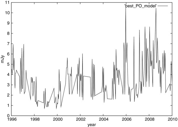
Figure 12. Flux distribution fs in the best PO model out of 106 trials.
Download figure:
Standard image High-resolution image
Figure 13. χ2s distribution in the PO model.
Download figure:
Standard image High-resolution imageThe statistical tests for the different cases are summarized in Table 1. Note that the detailed agreement of the test values for the best PO model and for the 1995 model is purely accidental.
Table 1. Correlations: Best of 106 Trials
| Correlated Quantities | χ2s | P(χ2s) | rs |
|---|---|---|---|
| Obs vs. α = 1 model | 310 | 6 × 10⁻⁴ | 0.30 |
| Obs vs. α = 2 model | 305 | 10−3 | 0.32 |
| Obs vs. QPO model | 290 | 7 × 10⁻³ | 0.37 |
| Obs vs. PO model | 205 | 0.9 | 0.58 |
Download table as: ASCIITypeset image
5. DISCUSSION
Figures 3–5 show the residuals of observations minus the 1995 model. The rms variability range is 1.4 mJy around the mean. It is not obvious that there is anything of significance in the scatter, except that we confirm the constant low-level variability of OJ287. The only possibly significant feature in the residuals is the 44 day periodicity which has been reported earlier from a smaller data set (Wu et al. 2006). The mean values of the residuals have been calculated assuming different periods from 0.08 yr (2 bins) to 0.52 yr (13 bins). The maximal amplitudes for each period (bin number) have been plotted in Figure 14. The figure shows peaks at the 44 day period and at its multiples. Valtonen et al. (2010) associate this period with the half-period of the innermost stable orbit of the accretion disk.

Figure 14. Maximum amplitude in the periodic variations of the light curve when the period is 2–13 bins long. One bin is 0.04 yr. The 44 day periodicity and its multiples are seen.
Download figure:
Standard image High-resolution image
The 1995 model made no effort to explain the small timescale variability shown in the residuals. It was well known from the light curve prior to 1995 that the low-level variability is always there, even after we take out the major predicted outbursts. Thus, it is no surprise to see this variability also during the period 1996–2010. Unlike Villforth et al. (2010), we do not think that the remaining peaks in Figures 3– 5 have any deep significance. These authors cited several of the residual peaks as evidence of the failure of the binary model. In our opinion, this is an overinterpretation of the 1995 model.
The only deviation from the 1995 model may be the deep flux decline in early 2008. There was a prediction of such a trough in the model, but it should have come 0.5 yr later. While in 1989 the secondary was 10° from the pole of the accretion disk during the fade, the 2008 fade occurs when the secondary is also 10° from the pole, but on the other side of it, according to the latest model (Valtonen et al. 2010). However, these figures refer to the mean pole of the disk which itself wobbles due to the binary action. The wobble of the jet is directly observed as a changing position angle of the radio jet; the change has been more than 40° around the year 2000 (Valtonen et al. 2011). Incidentally, the same wobble may be responsible for the increase of the base level of emission around that year (Valtonen 2007). These questions require further studies. The expected 1998 fade does not show up prominently with our time resolution; it has been described elsewhere (Valtonen et al. 1999).
There were only five outbursts that were clearly predicted; all five have now been observed, and what is left over could easily be described as random noise. It is seldom the case in astronomy that models perform better than this.
We thank Kari Nilsson for providing us with observational data files and valuable comments on the manuscript and the referee for comments which have considerably improved the paper.