


ABSTRACT
As part of an effort to study gas-grain chemical models in star-forming regions as they relate to molecules containing cyanide (–C≡N) groups, we present here a search for the molecules 2-cyanoethanol (OHCH2CH2CN) and methoxyacetonitrile (CH3OCH2CN) in the galactic center region SgrB2. These species are structural isomers of each other and are targeted to investigate the cross-coupling of pathways emanating from the photolysis products of methanol and ammonia with pathways involving cyano-containing molecules. Methanol and ammonia ices are two of the main repositories of the elements C, O, and N in cold clouds and understanding their link to cyanide chemistry could give important insights into prebiotic molecular evolution. Neither species was positively detected, but the upper limits we determined allow comparison to the general patterns gleaned from chemical models. Our results indicate the need for an expansion of the model networks to better deal with cyano-chemistry, in particular with respect to pathways including products of methanol photolysis. In addition to these results, the two main observational routes for detecting new interstellar molecules are discussed. One route is by decreasing detection limits at millimeter wavelength through spatial filtering with interferometric studies at the Atacama Large Millimeter Array (ALMA), and the second is by searching for intense torsional states at THz frequencies using the Herschel Space Observatory. 2-cyanoethanol and methoxyacetonitrile would both be good test beds for exploring the capabilities of ALMA and Herschel in the study of complex interstellar chemistry.
Export citation and abstract BibTeX RIS
1. INTRODUCTION
It has become increasingly clear in recent years that the inclusion of a variety of different pathways and processes is needed to give a coherent explanation of the patterns of complex organic chemistry seen in the dense cores of molecular clouds where stars are born. Beyond the gas phase and solid-state dust grain chemical pathways in quiescent clouds that have been the subject of study for nearly four decades (van Dishoeck & Blake 1998; Bergin & Tafalla 2007), the driving potential of both UV photons and highly energetic cosmic rays and the coupling between gas phase and solid state processes need to be considered. In particular, it has become clear that the coupling between gas phase and dust grain chemistry is stronger and more complex than previously thought. Instead of two largely independent reservoirs with a sudden onset of coupling when the star "switches on" and dust grain volatiles enter the gas phase, the warming of the dust grains as the star is being formed is likely a more gradual event that steadily increases the temperature of the dust grains, affecting both the chemistry in and on the grain and the coupling between solid and gas phases (Garrod & Herbst 2006; Garrod et al. 2008). A slower, more gradual increase of the grain temperature allows increased mobility and reactivity of a variety of chemical species, resulting in an increased opportunity for chemical maturation of dust grain mantles prior to entering into the gas phase. Ongoing waves of star formation can mix the material from one region of dense clouds to another, further driving the levels of molecular complexity that can be attained long before planetary surfaces are made.
Furthermore, even the "simple" solid-state dust grain chemistry in isolated, cold dense clouds is no longer thought to be limited to the tunneling of mobile hydrogen atoms through the barriers associated with stable molecules such as carbon monoxide (and the subsequent reaction with additional atoms; Charnley 2001), but to also include low-energy cosmic-ray driven processes. The energies of these particles, ∼MeV to hundreds of MeV, are too high to couple directly to the chemistry on dust grains, but their collision with a dust grain can release a cascade of thermal electrons at milder energies (∼keV) that have been experimentally shown to be capable of affecting ice mantle chemistry by cleaving molecular bonds and creating reactive intermediates that can then form new species (Bennet & Kaiser 2007). In addition, collisions between cosmic rays and molecular hydrogen can transfer kinetic energy from the cosmic ray into electronic degrees of freedom of H2, which can subsequently re-emit this energy in the form of UV photons (Prasad & Tarafdar 1983; Shen et al. 2004; Öberg et al. 2009). This secondary UV field can process ice in a similar way to direct cosmic-ray collisions, as the UV photons can cleave molecular bonds and create radical species (Öberg et al. 2009). The radical species formed through these processes can then react with each other (and with species formed through traditional tunneling processes) either in the pores left behind in the ice as the cosmic ray travels through the dust grain (Grieves & Orlando 2005), or as they become mobile with increasing grain temperature (Garrod & Herbst 2006; Öberg et al. 2009).
Chemical models of star-forming regions that include such processes and a gradual rather than sudden heating have shown general qualitative agreement with observational results, and in particular have proven capable of predicting the abundance ratios of molecular isomers that were previously difficult to explain with either gas phase reaction networks alone or the "prompt" injection of simple, first generation icy grain mantle products into the gas phase (Garrod & Herbst 2006; Garrod et al. 2008). In addition, laboratory studies on the processing of mixed ices with supra-thermal electrons (Bennet & Kaiser 2007) and UV photons (Öberg et al. 2009) have provided experimental support that boosts the new models. These combined results show that cosmic-ray-driven activation followed by diffusion and reaction as the ice heats up are likely to play a crucial role in the complex organic chemistry of star-forming regions. The next step in modeling the chemistry will be to expand the set of species and reactions included in these studies and the systematic comparison of observational results for structurally related molecules.
The first generations of the warm-up chemical models were limited to pathways involving small radical species resulting from bond cleavage of the major ice components H2O, H2CO, CH3OH, and NH3, as well as hydrogen tunneling additions to CO (Garrod et al. 2008). Since larger reactive species formed through cosmic ray and UV processing of ice species should also participate in grain mantle chemistry, a more recent version of these models featured an expanded set of pathways including larger reactive species (Belloche et al. 2009). In particular, detections of the cyano-molecules aminoacetonitrile (NH2CH2CN; Belloche et al. 2008a) and n-propyl cyanide (CH3CH2CH2CN; Belloche et al. 2009) have prompted the expansion of a subset of pathways to more closely focus on cyanide chemistry. In these latest models, various pathways emanating from either CN or larger radicals containing a cyanide group were included in an attempt to explain the observed relative abundances of these and previously observed cyano-molecules. Allowing CN to attach to larger hydrocarbons significantly overpredicted the abundances of thus formed species, and it was concluded that the incorporation of CN into the growing structure is one of the first steps in the pathway (Belloche et al. 2009). It was noted in that work, however, that the hydrocarbon network in the model was incomplete, which may make later incorporation of CN more relevant as this part of the model is updated (Belloche et al. 2009).
In this study, we investigate further expanding the set of potential pathways involving species containing a cyanide group by searching for the molecules 2-cyanoethanol (OHCH2CH2CN) and methoxyacetonitrile (CH3OCH2CN), and compare the search results with the abundances of other cyano-containing molecules seen in dense molecular clouds. The rotational spectra of both 2-cyanoethanol and methoxyacetonitrile were recently characterized (Braakman & Blake 2010a, 2010b) and are used as the basis for these observational searches. In addition, potential chemical pathways and expected abundances are discussed and compared with observational and theoretical results.
2. CYANO-CHEMISTRY
In the models discussed in Belloche et al. (2009), both aminoacetonitrile and n-propyl cyanide are suggested to be predominantly formed in pathways starting from CH2CN by addition of the NH2 radical in the case of aminoacetonitrile and by the sequential addition of CH2 and CH3 in the case of n-propyl cyanide. To test these models, we consider these pathways in a broader chemical context. In particular, we focus here on the potential cross-linking of these pathways with the products of cosmic ray and UV induced photoionization of methanol. If the assumed pathways to aminoacetonitrile and n-propyl cyanide (Belloche et al. 2009) are correct, then such cross-linking would seem likely as methanol is one of the major components of the ice mantles of interstellar dust grains. The two most likely pathways emanating from CH2CN and cross-linked with methanol derivatives would be (the reaction with NH2 is also shown for comparison):


The two structural isomers formed in reactions (1) and (2), methoxyacetonitrile (CH3OCH2CN) and cyanoethanol (OHCH2CH2CN), therefore make for good subjects to test the latest generation of grain mantle models, as their relative ratio should be a reflection of the ratio of the photolysis/cosmic ray dissociation products of methanol. Recent detailed studies on the photo-processing of interstellar ice analogs containing methanol indicate that the dominant products CH2OH and CH3O are formed at a ratio of approximately CH2OH:CH3O ∼ 5:1 (Öberg et al. 2009). In addition, the abundances of ammonia and methanol in interstellar ices are generally found to be within a factor of a few of each other (Schutte et al. 1991; Lacy et al. 1998; Dartois et al. 2002; Boogert et al. 2008; Bottinelli et al. 2010). Finally, to determine what abundance ratios we might expect from these three competing pathways, we need to consider the relative mobility of the radicals reacting with CH2CN. The estimated diffusion barriers are 1250 K for CH3O, 1978 K for NH2, and 2254 K for CH2OH (Garrod et al. 2008). Following Hasegawa et al. (1992), we can then calculate relative diffusion rates using D  , where m is the mass of the particle and Eb is the diffusion barrier (Hasegawa et al. 1992). With the numbers above, this gives D
 :
: :
: ∼ 1:326:3.9 × 10⁸ at 50 K and ∼ 1:21:1.7 × 10⁴ at 100 K. We see that CH3O is several orders of magnitude more mobile than both CH2OH and NH2 as dust grains warm-up, and based on this simple analysis we might therefore expect methoxyacetonitrile to be the most abundant product of the three reactions shown above. However, as mentioned in Garrod et al. (2008), the much increased diffusion rates of certain species can actually cause them to be depleted at early times and thus under-represented in reactions involving larger species that only become mobile at later times and higher dust temperatures. Indeed, the models predict that for highly mobile reaction partners (HCO, CH3O) the CH3O species have a higher abundance than CH2OH species, and dimethyl ether (CH3OCH3) and methyl formate (HCOOCH3) are the most important repositories for CH3O reactions, both results that qualitatively agree with observational results in SgrB2 and OMC-1 (Garrod et al. 2008; Sutton et al. 1995). This also successfully explains the previously puzzling observation that methyl formate has a much higher observed abundance than its isomers acetic acid (CH3COOH) and glycolaldehyde (CH2OHCHO; Hollis et al. 2001; Garrod & Herbst 2006). For larger and less mobile reaction partners, especially with the CH3O/CH2OH pair, observational results are largely absent, at least in part due to the lower abundance of larger species. The observations pursued here would thus provide an important test of the basic assumptions in chemical models.
The different binding energies of these three species on the grain should also affect their relative gas-phase abundances as more strongly bound species evaporate at higher temperatures and thus later times. The OH group in cyanoethanol can both donate and accept hydrogen bonds and should be the most strongly bound of the three species. The slightly lower electronegativity of nitrogen results in somewhat weaker hydrogen bonds for the NH2 group in aminoacetontrile (again both donating and accepting) and finally the lone pair electrons of the oxygen atom in methoxyacetonitrile can only accept hydrogen bonds. Looking at the predictions in the models by Garrod et al. (2008), we see that –CH2OH species generally peak at the highest temperatures, followed by –NH2 and –OCH3 species at similar temperatures somewhat below this (Garrod et al. 2008). Other potential processes may also affect the abundances of these molecules, including alternative formation as well as destruction pathways that might favor one over another of these species. To completely resolve the expected abundance ratios a full-scale model would be needed. Indeed, systematic expansion of chemical models toward larger and more complex species would allow for more quantitative statements on the chemistry considered here. More generally, in the future this should become one of the main paths toward better understanding the complex chemistry in star-forming regions, particularly as observational data from next generation telescopes such as the Herschel Space Observatory and the Atacama Large Millimeter Array (ALMA) becomes available. Nonetheless, the searches in this study represent a qualitative test of the assumptions in warm-up chemical models, as well as a qualitative first attempt at investigating whether species as complex as methoxyacetonitrile and 2-cyanoethanol can be detected at millimeter-wave frequencies using ground-based single dish telescopes.
3. OBSERVATIONS AND DATA ANALYSIS
The two hot core regions Sgr B2(N) and Sgr B2(M) were observed with the IRAM 30 m telescope on Pico Valeta, Spain, over the course of a year, in 2004 January, 2004 September, and 2005 January. A complete spectral survey of the 3 mm atmospheric window from 80 to 116 GHz was carried out, along with associated surveys in the 1.3 mm window between 201.8 and 204.6 GHz and between 205.0 and 217.7 GHz. Selected spectra in the 2 mm window and 1 mm window between 219 and 268 GHz were also obtained. The coordinates of the observed position for Sgr B2(N) are αJ2000 = 17h47m20 0, δJ2000 = −28 °22'19
 0 with a systemic velocity Vlsr = 64 km s−1 and αJ2000 = 17h47m204, δJ2000 = −28 °23'070 with a systemic velocity Vlsr = 62 km s−1 for Sgr B2(M). Additional details about the observational setup and data reduction can be found in Belloche et al. (2008a). An rms noise level of 15–20 mK on the T⋆a scale was achieved below 100 GHz, 20–30 mK between 100 and 114.5 GHz, about 50 mK between 114.5 and 116 GHz, and 25–60 mK in the 2 mm atmospheric window. At 1.3 mm, the confusion limit was reached for most of the spectra obtained toward Sgr B2(N).
A central goal of the survey was to characterize as best as possible the molecular content of Sgr B2(N) and (M). The careful modeling of the emission of all known molecules in detail also facilitates the search for new species. The broadband nature of the data allows this to be done with high accuracy, because the emission of a target molecule can be modeled and compared with the observational data over the entire frequency space using a global model of known molecules as a reference. Claiming a detection of a new molecule is thus possible if all lines emitted by the target species are present in the data at the right intensity according to the model. The absence of even a single line in the observed spectrum signifies a non-detection for the species in question. In this case, an upper limit on the column density can be determined using the noise (or confusion) level at the line positions accurately known from previous laboratory work. The emission of both the known molecules and new targets are modeled using the XCLASS software5 in the local thermodynamic equilibrium (LTE) approximation, with source size, temperature, column density, velocity line width, and velocity offset with respect to the systemic velocity of the source as the free parameters (for more details on the modeling and analysis see Belloche et al. 2008a, 2009).
The full millimeter-wave rotational spectra of both methoxyacetonitrile and cyanoethanol were recently characterized (Braakman & Blake 2010a, 2010b), and these results were used as the basis for the observational study here. For both molecules the gauche conformer is lowest in energy by a significant margin over the next lowest conformer, 5.7 kJ mol−1 in the case of methoxyacetonitrile (Kewley 1974) and 2.7 kJ mol−1 in the case of cyanoethanol (Marstokk & Mollendal 1985). These conformers are therefore the focus of the present observational searches toward Sgr B2.
Both molecules have large dipole moments (μa = 1.8 D and μb = 2.5 D for cyanoethanol, μa = 2.4 D and μb = 1.4 D for methoxyacetonitrile) resulting in exceptionally rich and dense spectra. Because these molecules are strongly prolate tops (κ = −0.844 for cyanoethanol and κ = −0.878 for methoxyacetonitrile) and effects of internal rotation are absent (or unimportant), both species are well-behaved asymmetric tops and their spectra can be accurately described using the parameters shown in Table 1. The rotational partition function merits some extra attention here due to the fact that both molecules have several low-lying torsional states in the ∼75–200 cm−1 range (Kewley 1974; Marstokk & Mollendal 1985). These states are significantly populated at room temperature and their inclusion in the partition function is known to be important in correctly modeling the room temperature spectra of both molecules (Braakman & Blake 2010a, 2010b). Although the rotational excitation temperatures of typical hot core molecules are significantly lower than the 300 K conditions under which the laboratory spectra were measured and these states are thus unlikely to be detected, the inclusion of the excited torsional states has a significant impact on the magnitude of the partition function even at these temperatures. For example, the partition function for methoxyacetonitrile is 4.716 × 10⁴ and 1.216 × 10⁴ at 150 and 75 K, respectively, numbers that would be reduced to 2.864 × 10⁴ and 1.013 × 10⁴ if excited torsional states are not considered. For cyanoethanol, the partition function is 5.371 × 10⁴ and 1.265 × 10⁴ at 150 and 75 K, respectively (3.042 × 10⁴ and 1.076 × 10⁴ if the far-infrared torsional states are excluded).
Table 1. Spectroscopic Parameters of Cyanoethanol and Methoxyacetonitrile
| Parameter (Units) | Value (Unc.) | |
|---|---|---|
| Cyanoethanol | Methoxyacetonitrile | |
| A (MHz) | 10726.45630(108) | 11893.73683(123) |
| B (MHz) | 3432.310915(279) | 3423.36198(41) |
| C (MHz) | 2815.606794(305) | 2871.47309(42) |
| −ΔJ(kHz) | 4.878082(108) | 3.424161(272) |
| −ΔJK(kHz) | −29.02150(101) | −23.90946(91) |
| −ΔK(kHz) | 80.2471(48) | 101.0630(56) |
| −δJ(kHz) | 1.4945691(280) | 1.061232(88) |
| −δK(kHz) | 10.56645(109) | 10.4079(46) |
| HJ(Hz) | 0.0147946(138) | 0.006565(85) |
| HJK(Hz) | 0.070757(301) | 0.05723(133) |
| HKJ(Hz) | −1.09796(143) | −1.0446(49) |
| HK(Hz) | 2.9708(85) | 4.2132(79) |
| hJ(Hz) | 0.0067636(35) | 0.0027027(178) |
| hJK(Hz) | −0.017433(191) | −0.03933(118) |
| hK(Hz) | 1.46446(266) | 1.3265(309) |
| LJ(mHz) | −0.0000802(101) | |
| LJK(mHz) | −0.0007870(214) | |
| LJJK(mHz) | −0.011141(173) | 0.010014(162) |
| LKJ(mHz) | 0.07166(45) | 0.07135(38) |
| LK(mHz) | −0.1445(48) | |
Download table as: ASCIITypeset image
4. UPPER LIMITS OF METHOXYACETONITRILE AND CYANOETHANOL
We searched for methoxyacetonitrile and cyanoethanol toward Sgr B2(N) by modeling their emission spectra in the LTE approximation. Since both molecules are supposed to share a common chemical pathway with aminoacetonitrile to some extent and are of similar complexity as the latter, we modeled their emission based on the parameters derived for aminoacetonitrile by Belloche et al. (2008a): an angular source size of 2'', an excitation temperature of 100 K, a line width (FWHM) of 7 km s−1, and no velocity offset with respect to the systemic velocity of the source. We call this set of parameters the reference model. We also investigated alternative models, one with the same parameters but a higher temperature (200 K), and one with an extended cold emission (60'' and 15 K, see Hollis et al. 2004).
Most transitions of cyanoethanol and methoxyacetonitrile are expected to be heavily blended with stronger emission from other species. Based on the reference model, Tables 6 and 7 in the Appendix list all transitions predicted to be stronger than a very conservative threshold of 20 mK (in main-beam temperature scale). The last column of these tables lists the blends affecting each transition. A few transitions or group of transitions (which we call "features") of each molecule suffer less from blending and are marked in bold face. These are the only transitions that can a priori be used to claim a detection or derive a column density upper limit toward Sgr B2(N). Some of these features are tentatively detected or at least consistent with the observations. They are marked "candidate" in the last column of Tables 6 and 7. However, a few other features are apparently missing in the observed spectrum and are marked "missing."
All these "candidate" and "missing" features, 8 for methoxyacetonitrile and 17 for cyanoethanol, are listed with more details in Tables 2 and 3. A feature consists of one transition, or several transitions that are so close to each other that they cannot be spectrally resolved or they significantly overlap in our single-dish spectrum of Sgr B2(N). The features are labeled in Column 8 of each table. The peak opacity and integrated intensity of each modeled feature are listed in Columns 9 and 11, respectively. The frequency range for the integration was based on the model prediction (down to roughly 10% of the model peak temperature). The observed integrated intensity (Column 10) was computed on the same frequency range. Column 12 provides the intensity integrated over the same frequency range for the complete model that contained all species identified in our spectrum of Sgr B2(N) so far. This represents the amount of contamination of the possible emission of methoxyacetonitrile and cyanoethanol by other species. All "candidate" and "missing" features of methoxyacetonitrile and cyanoethanol toward Sgr B2(N) are displayed in Figures 1 and 2, respectively. The spectrum of Sgr B2(M) is also shown for comparison.

Figure 1. Transitions of the gauche conformer of methoxyacetonitrile (CH3OCH2CN–g) tentatively detected with the IRAM 30 m telescope or missing. Each panel consists of two plots and is labeled in black in the upper right corner. The lower plot shows in black the spectrum obtained toward Sgr B2(N) in main-beam brightness temperature scale (K), while the upper plot shows the spectrum toward Sgr B2(M). The rest-frequency axis is labeled in GHz. The systemic velocities assumed for Sgr B2(N) and (M) are 64 and 62 km s−1, respectively. The lines identified in the Sgr B2(N) spectrum are labeled in blue. The top red label indicates the CH3OCH2CN–g transition centered in each plot (numbered like in Column 1 of Table 2), along with the energy of its lower level in K (El/kB). The bottom red label is the feature number (see Column 8 of Table 2). The green spectrum shows our LTE model containing all identified molecules, but not CH3OCH2CN–g. The LTE synthetic spectrum of CH3OCH2CN–g alone is overlaid in red, and its opacity in dashed violet. All observed lines which have no counterpart in the green spectrum are still unidentified in Sgr B2(N).
Download figure:
Standard image High-resolution image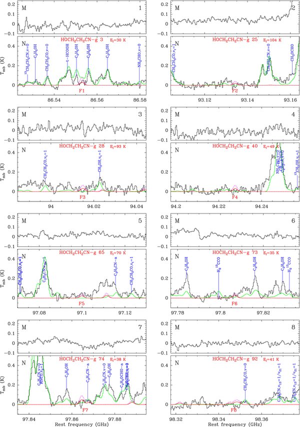
Download figure:
Standard image High-resolution image
Download figure:
Standard image High-resolution image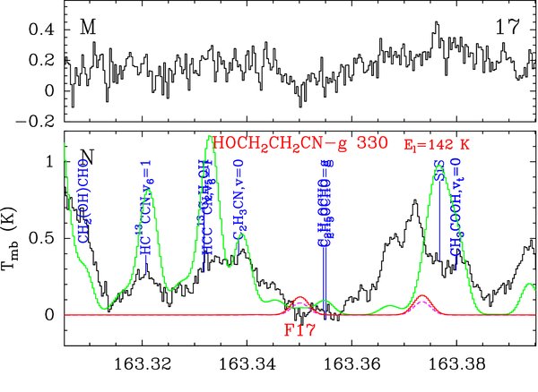
Figure 2. Transitions of the gauche conformer of 2-cyanoethanol (HOCH2CH2CN–g) tentatively detected with the IRAM 30 m telescope or missing. Each panel consists of two plots and is labeled in black in the upper right corner. The lower plot shows in black the spectrum obtained toward Sgr B2(N) in main-beam brightness temperature scale (K), while the upper plot shows the spectrum toward Sgr B2(M). The rest frequency axis is labeled in GHz. The systemic velocities assumed for Sgr B2(N) and (M) are 64 and 62 km s−1, respectively. The lines identified in the Sgr B2(N) spectrum are labeled in blue. The top red label indicates the HOCH2CH2CN–g transition centered in each plot (numbered like in Column 1 of Table 3), along with the energy of its lower level in K (El/kB). The bottom red label is the feature number (see Column 8 of Table 3). The green spectrum shows our LTE model containing all identified molecules, but not HOCH2CH2CN–g. The LTE synthetic spectrum of HOCH2CH2CN–g alone is overlaid in red, and its opacity in dashed violet. All observed lines which have no counterpart in the green spectrum are still unidentified in Sgr B2(N).
Download figure:
Standard image High-resolution image
Table 2. Transitions of the Gauche Conformer of Methoxyacetonitrile Tentatively Detected or Missing Toward Sgr B2(N) with the IRAM 30 m Telescope
| Na | Transition | Frequency | Unc.b | Elc | Sμ2 | σd | Fe | τf | Iobsg | Imodg | Iallg | Comments |
|---|---|---|---|---|---|---|---|---|---|---|---|---|
| (MHz) | (kHz) | (K) | (D2) | (mK) | (K km s−1) | (K km s−1) | ||||||
| (1) | (2) | (3) | (4) | (5) | (6) | (7) | (8) | (9) | (10) | (11) | (12) | (13) |
| 3 | 136,8–126,7 | 82154.546 | 8 | 39 | 59 | 19 | 1 | 0.06 | 0.16(08) | 0.19 | 0.14 | Candidate group, partial blend |
| with CH3CH3CO, vt = 1 | ||||||||||||
| 4 | 136,7–126,6 | 82154.817 | 8 | 39 | 59 | 19 | 1 | ... | ... | ... | ... | ... |
| 22 | 146,9–136,8 | 88516.044 | 8 | 43 | 66 | 17 | 2 | 0.07 | 0.65(07) | 0.25 | 0.37 | Candidate group, partial blend |
| with C2H5CN, v13 = 1/v21 = 1 | ||||||||||||
| and H13CCCN, v7 = 1 | ||||||||||||
| 23 | 146,8–136,7 | 88516.682 | 8 | 43 | 66 | 17 | 2 | ... | ... | ... | ... | ... |
| 41 | 157,9–147,8 | 94781.913 | 8 | 52 | 68 | 28 | 3 | 0.07 | 0.44(12) | 0.29 | 0.01 | Candidate group |
| 42 | 157,8–147,7 | 94781.948 | 8 | 52 | 68 | 28 | 3 | ... | ... | ... | ... | ... |
| 73 | 169,7–159,6 | 101013.914 | 9 | 70 | 63 | 21 | 4 | 0.06 | 0.65(08) | 0.28 | 0.21 | Candidate group, partial blend |
| with U-line, and | ||||||||||||
| CH3CH3CO, vt = 1 | ||||||||||||
| 74 | 169,8–159,7 | 101013.914 | 9 | 70 | 63 | 21 | 4 | ... | ... | ... | ... | ... |
| 75 | 315,27–306,25 | 101015.693 | 19 | 157 | 7 | 21 | 4 | ... | ... | ... | ... | ... |
| 80 | 166,11–156,10 | 101267.615 | 8 | 51 | 79 | 21 | 5 | 0.05 | 0.32(10) | 0.42 | 0.07 | Candidate group, uncertain |
| baseline | ||||||||||||
| 81 | 166,10–156,9 | 101270.538 | 8 | 51 | 79 | 21 | 5 | ... | ... | ... | ... | ... |
| 84 | 164,13–154,12 | 101600.336 | 8 | 43 | 86 | 16 | 6 | 0.06 | −0.03(06) | 0.25 | 0.01 | Missing line, but uncertain |
| baseline? | ||||||||||||
| 127 | 175,12–165,11 | 108003.802 | 9 | 52 | 89 | 46 | 7 | 0.06 | 0.46(17) | 0.28 | 0.08 | Candidate line, noisy |
| 137 | 183,16–173,15 | 113023.465 | 9 | 50 | 100 | 40 | 8 | 0.07 | −0.04(15) | 0.37 | 0.57 | Missing line, but uncertain |
| baseline? | ||||||||||||
Notes. aNumbering of the observed transitions associated with a modeled line stronger than 20 mK (see Table 6). bFrequency uncertainty. cLower-energy level in temperature units (El/kB). dCalculated rms noise level in Tmb scale. eNumbering of the candidate or missing features. fPeak opacity of the modeled feature. gIntegrated intensity in Tmb scale for the observed spectrum (Column 10), the methoxyacetonitrile model (Column 11), and the model including all molecules except methoxyacetonitrile (Column 12). The uncertainty in Column 10 is given in parentheses in units of the last digit.
Download table as: ASCIITypeset image
Table 3. Transitions of the Gauche Conformer of 2-Cyanoethanol Tentatively Detected or Missing Toward Sgr B2(N) with the IRAM 30 m Telescope
| Na | Transition | Frequency | Unc.b | Elc | Sμ2 | σd | Fe | τf | Iobsg | Imodg | Iallg | Comments |
|---|---|---|---|---|---|---|---|---|---|---|---|---|
| (MHz) | (kHz) | (K) | (D2) | (mK) | (K km s−1) | (K km s−1) | ||||||
| (1) | (2) | (3) | (4) | (5) | (6) | (7) | (8) | (9) | (10) | (11) | (12) | (13) |
| 3 | 150,15–141,14 | 86552.902 | 8 | 30 | 85 | 17 | 1 | 0.08 | 0.48(07) | 0.25 | 1.43 | Candidate group, blend with |
| C2H5OH, uncertain baseline | ||||||||||||
| 4 | 2517,8–2616,11 | 86554.133 | 15 | 199 | 6 | 17 | 1 | ... | ... | ... | ... | ... |
| 5 | 2517,9–2616,10 | 86554.133 | 15 | 199 | 6 | 17 | 1 | ... | ... | ... | ... | ... |
| 25 | 247,17–246,18 | 93134.179 | 11 | 104 | 87 | 22 | 2 | 0.04 | 0.10(09) | 0.15 | 0.01 | Missing line, but noisy and |
| uncertain baseline? | ||||||||||||
| 28 | 1513,2–1413,1 | 94014.420 | 7 | 93 | 13 | 31 | 3 | 0.07 | 0.31(13) | 0.27 | 0.02 | Missing group, uncertain |
| baseline? | ||||||||||||
| 29 | 1513,3–1413,2 | 94014.420 | 7 | 93 | 13 | 31 | 3 | ... | ... | ... | ... | ... |
| 30 | 287,22–286,23 | 94014.809 | 11 | 136 | 106 | 31 | 3 | ... | ... | ... | ... | ... |
| 31 | 1512,3–1412,2 | 94015.384 | 7 | 84 | 18 | 31 | 3 | ... | ... | ... | ... | ... |
| 32 | 1512,4–1412,3 | 94015.384 | 7 | 84 | 18 | 31 | 3 | ... | ... | ... | ... | ... |
| 40 | 157,9–147,8 | 94227.567 | 7 | 49 | 40 | 26 | 4 | 0.06 | 0.11(11) | 0.25 | 0.09 | Missing group, but uncertain |
| baseline? | ||||||||||||
| 41 | 157,8–147,7 | 94227.738 | 7 | 49 | 40 | 26 | 4 | ... | ... | ... | ... | ... |
| 65 | 197,13–196,14 | 97099.887 | 10 | 70 | 63 | 21 | 5 | 0.04 | 0.52(08) | 0.17 | 0.00 | Candidate line, blend with |
| U-line? | ||||||||||||
| 73 | 153,12–143,11 | 97806.800 | 7 | 35 | 49 | 20 | 6 | 0.05 | 0.50(08) | 0.20 | 0.18 | Candidate line, blend with |
| C2H5CN, v13 = 1/v21 = 1 and | ||||||||||||
| C2H5OH | ||||||||||||
| 74 | 170,17–161,16 | 97864.630 | 8 | 38 | 98 | 20 | 7 | 0.09 | 0.62(10) | 0.54 | 0.63 | Missing group, blend with |
| C3H7CN | ||||||||||||
| 75 | 167,10–166,10 | 97867.370 | 11 | 54 | 1 | 20 | 7 | ... | ... | ... | ... | ... |
| 76 | 167,9–166,10 | 97868.051 | 11 | 54 | 50 | 20 | 7 | ... | ... | ... | ... | ... |
| 92 | 137,7–136,7 | 98347.596 | 11 | 41 | 1 | 18 | 8 | 0.05 | −0.07(10) | 0.40 | 0.14 | Missing group, blend with |
| U-line and CH3CH3CO, | ||||||||||||
| uncertain baseline | ||||||||||||
| 93 | 137,6–136,7 | 98347.629 | 11 | 41 | 36 | 18 | 8 | ... | ... | ... | ... | ... |
| 94 | 137,7–136,8 | 98349.265 | 11 | 41 | 36 | 18 | 8 | ... | ... | ... | ... | ... |
| 95 | 137,6–136,8 | 98349.298 | 11 | 41 | 1 | 18 | 8 | ... | ... | ... | ... | ... |
| 123 | 169,8–159,7 | 100379.093 | 7 | 66 | 37 | 24 | 9 | 0.05 | 0.02(10) | 0.24 | 0.17 | Candidate group, blend with |
| CH3CH3CO, vt = 1, uncertain | ||||||||||||
| baseline | ||||||||||||
| 124 | 169,7–159,6 | 100379.093 | 7 | 66 | 37 | 24 | 9 | ... | ... | ... | ... | ... |
| 127 | 167,10–157,9 | 100564.513 | 7 | 54 | 44 | 20 | 10 | 0.07 | 0.31(08) | 0.31 | 0.08 | Missing group, uncertain |
| baseline? | ||||||||||||
| 128 | 167,9–157,8 | 100564.925 | 7 | 54 | 44 | 20 | 10 | ... | ... | ... | ... | ... |
| 137 | 162,14–152,13 | 102456.406 | 7 | 39 | 53 | 30 | 11 | 0.05 | 0.36(12) | 0.24 | 0.37 | Candidate line, partial blend |
| with CH3CH3CO | ||||||||||||
| 138 | 164,12–154,11 | 102622.206 | 7 | 42 | 51 | 37 | 12 | 0.05 | 0.11(14) | 0.22 | 0.00 | Candidate line |
| 150 | 181,18–170,17 | 103555.237 | 8 | 43 | 104 | 27 | 13 | 0.10 | 0.93(11) | 0.45 | 0.24 | Candidate line, noisy |
| 174 | 179,9–169,8 | 106685.426 | 7 | 70 | 42 | 34 | 14 | 0.06 | −0.65(13) | 0.30 | 0.39 | Missing group, blend with |
| CH3CH3CO, uncertain baseline | ||||||||||||
| 175 | 179,8–169,7 | 106685.426 | 7 | 70 | 42 | 34 | 14 | ... | ... | ... | ... | ... |
| 189 | 182,17–172,16 | 107863.000 | 8 | 46 | 60 | 46 | 15 | 0.06 | −0.02(17) | 0.29 | 0.15 | Candidate line, blend with |
| C3H7CN, noisy | ||||||||||||
| 245 | 198,12–197,12 | 112858.588 | 11 | 75 | 1 | 40 | 16 | 0.05 | 2.18(17) | 0.53 | 0.13 | Missing group, uncertain |
| baseline? | ||||||||||||
| 246 | 198,11–197,12 | 112858.852 | 11 | 75 | 59 | 40 | 16 | ... | ... | ... | ... | ... |
| 247 | 1812,6–1712,5 | 112861.107 | 8 | 98 | 34 | 40 | 16 | ... | ... | ... | ... | ... |
| 248 | 1812,7–1712,6 | 112861.107 | 8 | 98 | 34 | 40 | 16 | ... | ... | ... | ... | ... |
| 249 | 1816,2–1716,1 | 112861.973 | 8 | 139 | 13 | 40 | 16 | ... | ... | ... | ... | ... |
| 250 | 1816,3–1716,2 | 112861.973 | 8 | 139 | 13 | 40 | 16 | ... | ... | ... | ... | ... |
| 330 | 2611,16–2511,15 | 163350.130 | 8 | 142 | 73 | 38 | 17 | 0.08 | 0.83(12) | 0.88 | 1.03 | Missing group, blend with |
| C2H5OCHO, uncertain | ||||||||||||
| baseline? | ||||||||||||
| 331 | 2611,15–2511,14 | 163350.132 | 8 | 142 | 73 | 38 | 17 | ... | ... | ... | ... | ... |
Notes. aNumbering of the observed transitions associated with a modeled line stronger than 20 mK (see Table 7). bFrequency uncertainty. cLower energy level in temperature units (El/kB). dCalculated rms noise level in Tmb scale. eNumbering of the candidate or missing features. fPeak opacity of the modeled feature. gIntegrated intensity in Tmb scale for the observed spectrum (Col. 10), the 2-cyanoethanol model (Column 11), and the model including all molecules except 2-cyanoethanol (Column 12). The uncertainty in Column 10 is given in parentheses in units of the last digit.
Download table as: ASCIITypeset image
Three features of methoxyacetonitrile are tentatively detected (F2, F3, and F4), three have a too low signal-to-noise ratio but are consistent with the model (F1, F5, and F7), and two appear to be missing in the observed spectrum (F6 and F8). Although these two missing features are sufficient to invalidate a detection, it cannot be excluded that the baseline level was overestimated due to the high degree of line confusion around these features, especially for feature F8. As a result, we can consider our model as an upper limit to the detection of methoxyacetonitrile. The parameters of this reference model are listed in Table 4, along with the parameters of the two alternative models investigated in the same way.
Table 4. Column Density Upper Limits
| Cyanoethanol | |||
|---|---|---|---|
| Upper limit | |||
| Source | Source size | Trot | NT |
| SgrB2 | (K) | (cm−2) | |
| (N) | 2'' | 200 | 1 × 10¹⁷ |
| 2'' | 100 | 5 × 10¹⁶ | |
| 60'' | 15 | 8 × 10¹³ | |
| (M) | 2'' | 200 | 1 × 10¹⁷ |
| 2'' | 100 | 5 × 10¹⁶ | |
| 60'' | 15 | 6 × 10¹³ | |
| Methoxyacetonitrile | |||
| Upper limit | |||
| Source | Source size | Trot (K) | NT |
| SgrB2 | (K) | (cm−2) | |
| (N) | 2'' | 200 | 8 × 10¹⁶ |
| 2'' | 100 | 3 × 10¹⁶ | |
| 60'' | 15 | 1.2 × 10¹⁴ | |
| (M) | 2'' | 200 | 5 × 10¹⁶ |
| 2'' | 100 | 2.5 × 10¹⁶ | |
| 60'' | 15 | 4 × 10¹³ | |
Download table as: ASCIITypeset image
One feature of cyanoethanol is tentatively detected (F1, the contamination by ethanol being maybe somewhat overestimated), seven have a too low signal-to-noise ratio but are consistent with the model (F5, F6, F9, F11, F12, F13, and F15), and nine appear to be missing (F2, F3, F4, F7, F8, F10, F14, F16, and F17). Most of the missing features are actually very close to the noise level or suffer from a very uncertain baseline level. They do not clearly rule out a detection, but overall we can again only derive an upper limit (see Table 4).
As Table 4 shows, assuming a hot core emission angular size and a rotational temperature similar to that of aminoacetonitrile (2'' and 100 K), we find column density upper limits of 3 × 1016 cm−2 for methoxyacetonitrile and 5 × 1016 cm−2 for cyanoethanol in Sgr B2(N). Using an H2 column density of 1.7 × 1025 (Belloche et al. 2008b), this gives abundance upper limits relative to H2 of 1.8 × 10⁻⁹ for methoxacetonitrile and 2.9 × 10⁻⁹ for cyanoethanol. By comparison, aminoacetonitrile has an observed abundance of 1.7 × 10⁻⁹ (Belloche et al. 2008b).
5. DISCUSSION
In the present search for the molecules 2-cyanoethanol and methoxyacetonitrile, we cannot claim a detection based on the observational data. Several predicted spectral features for both molecules did match features in the observational data, but other features were not present leading to only upper limits being obtained. A closer inspection of the observational data indicates that although both species were not detected, the possibility exists that they may be only just below the detection limit. The high degree of line blending in some regions of the spectra can make it difficult to find the emission-free channels that are needed to establish the baseline against which the molecular fluxes are determined, which adds considerable uncertainty to the estimated line fluxes near the rms levels of the survey. Indeed, looking both in Figures 1 and 2 and the corresponding tables, in basically all cases where a line was found missing there was some uncertainty as to the true level of the baseline. If it were slightly lower for those regions where lines were found missing, the predicted spectra would still be compatible with the observational data. Furthermore, for most frequencies it is the emission from other, more abundant species that sets the confusion floor against which any new molecular features must be sought. In such cases, additional integration time or more sensitive detectors are of no use in improving the chances of detecting additional species in the star-forming cores of dense clouds.
What, then, is to be done? The Sgr B2(N) and (M) hot cores are among the highest column density regions known, but are quite distant (lying adjacent to the Galactic center) and are characterized by complex emission and absorption line profiles. Molecular line surveys toward additional hot cores, especially those with narrower emission line profiles (e.g., NGC 6334; Schilke et al. 2006), would be useful in determining whether the results obtained here apply more generally. Even so, single dish surveys, with their large beam sizes, necessarily blend the molecular features from a range of cloud environments. Thus, the present results provide yet another example of the power of interferometric observations in the search for new interstellar molecules. By combining the signals from many radio telescopes spread over a range of distributions on the ground, aperture synthesis observations allows for both higher and tailored spatial resolution of the data than is possible in single dish experiments, which has several advantages.
As was shown in the case of aminoacetonitrile (Belloche et al. 2008a), confirming that the emission of different transitions assigned to a newly detected molecule is indeed arises from the same spatial location provides a powerful verification of the detection. Furthermore, by concentrating on the longest baselines available in the interferometric data, it is possible to "filter out" the smooth molecular emission from more common species. In most sources this leads to a significant reduction in the line confusion. As interferometric observatories such as CARMA reach their full capabilities and, in particular, once ALMA comes online, the detection of larger molecules such as those searched for here, but that are severely hindered by line blending, may well become possible. For example, ALMA will consist of fifty 12 m antennas at a site markedly superior to that at Pico Valeta (or CARMA), and at full capacity will be able to achieve spatial resolutions on the order ∼ 001 at a wavelength of 1 mm. In comparison, CARMA and the eSMA can now achieve ∼ 02–03 resolution at 3 mm (Isella et al. 2010) and 0.87 mm (Shinnaga et al. 2009), respectively, whereas the interferometric studies at 3 mm in Belloche et al. (2008a) had resolutions of ∼ 34 × 08 (IRAM Plateau de Bure Interferometer) and ∼ 34 × 23 (Australia Compact Array Interferometer). The larger collecting area of ALMA will also result in an increase in raw sensitivity by a factor of ∼ 8 over the IRAM 30 m, and the ALMA correlator will be able to process 16 GHz of spectral line data in a single local oscillator setting. Thus, surveys at least a factor of ten deeper than those reported here will be possible in a matter of hours, and when searching for emission from compact hot cores the expectation is that the line confusion will be reduced by similar factors. As a result, ALMA will radically advance observational studies of existing and new interstellar molecules, as well as deepening our understanding of complex interstellar chemistry by constraining theoretical models.
Even in the absence of clean detections for methoxyacetonitrile and cyanoethanol, their upper limits measured here still give some information about grain mantle chemistry. The previously measured column density for aminoacetonitrile was 2.8 × 1016 cm−2 at a rotational temperature of 100 K. It should be noted that for aminoacetonitrile the contributions of excited states to the partition function were not taken into account. The lowest energy vibrational modes of this molecules lie at 237 cm−1 (C–CN bend), 247 cm−1 (NH2 torsion), and 370 cm−1 (NH2–CH2 torsion; Bernstein et al. 2004), which at 100 K increases the partition function by ∼ 7%. As a result the observed column density of aminoacetonitrile should be increased to 3.0 × 1016 cm−2. Assuming the same rotational excitation temperature (100 K) for the two species studied here, we find upper limits on their column densities of 3 × 1016 cm−2 for methoxyacetonitrile and 5 × 1016 cm−2 for cyanoethanol. It is thus likely that the abundance of methoxyacetonitrile lies below that of aminoacetonitrile. Cyanoethanol could still have an abundance similar to or above that of aminoacetonitrile, but the signal would have to be just barely below the noise/confusion level of the current study.
How do these results compare to general model predictions and what does this tell us about chemical pathways of cyano-molecule and their cross-coupling with ammonia and methanol pathways? To get further insights into this chemistry, we look more closely at the results of the models in Garrod et al. (2008). Table 4 in that work lists the predicted peak gas-phase abundances for a large variety of molecules, and we searched that set for groups of species differing only by the attached moieties NH2, CH2OH, and CH3OH (i.e., molecules of the form X–Y, where Y is NH2, CH2OH, or OCH3 and X is the same for all three), and compared their relative abundances. The resulting numbers are shown in Table 5, where for each reaction partner, X, and warm-up timescale, tw, the abundances are scaled relative to that of X–NH2, which is set to 1. The different warm-up timescales refer to high-mass (5 × 10⁴ yr), intermediate-mass (2 × 10⁵ yr) and low-mass (1 × 10⁶ yr) hot cores, respectively (Garrod & Herbst 2006).
Table 5. Predicted Peak Gas-phase Abundance Ratios in Hot Cores of Species Whose Composition Differ only by the Ammonia and Methanol Dissociation Products NH2, CH2OH, and CH3O
| tw (yr) | Species | X = CH3 | CH3CO | CH3O | COCHO | CH2OH | NH2CO | COOH | COCH2OH | CH2CNa |
|---|---|---|---|---|---|---|---|---|---|---|
| Eb (K) = 588 | 1163 | 1250 | 1375 | 2254 | 2553 | 2560 | 3117 | |||
| 5 × 10⁴ | H2N–X | 1.0 | 1.0 | 1.0 | 1.0 | 1.0 | 1.0 | 1.0 | 1.0 | 1.0 |
| HOCH2–X | 0.13 | 0.008 | 0.17 | 0.003 | 0.42 | 0.14 | 0.07 | 0.04 | <1.0 | |
| CH3O–X | 0.23 | 0.001 | 0.017 | 0.001 | 0.15 | 0.02 | 0.03 | 0.02 | <1.7 | |
| 2 × 10⁵ | H2N–X | 1.0 | 1.0 | 1.0 | 1.0 | 1.0 | 1.0 | 1.0 | 1.0 | |
| HOCH2–X | 0.14 | 0.021 | 0.15 | 0.014 | 0.08 | 0.07 | 0.06 | 0.04 | ||
| CH3O–X | 0.16 | 0.004 | 0.012 | 0.005 | 0.09 | 0.04 | 0.06 | 0.05 | ||
| 1 × 10⁶ | H2N–X | 1.0 | 1.0 | 1.0 | 1.0 | 1.0 | 1.0 | 1.0 | 1.0 | |
| HOCH2–X | 0.19 | 0.062 | 0.09 | 0.068 | 0.04 | 0.06 | 0.10 | 0.08 | ||
| CH3O–X | 0.09 | 0.008 | 0.003 | 0.026 | 0.09 | 0.04 | 0.04 | 0.05 |
Notes. Numbers adapted from Table 4 in Garrod et al. (2008) and scaled relative to the abundance of X–NH2 (which is set to 1.0) for each reaction partner X and different warm-up timescales (tw) for the hot core. The observed ratios for X–CH2CN are listed for comparison. aThe limits for CH2CN products are listed for the fastest warm-up time only as SgrB2(N) is a high-mass source.
Download table as: ASCIITypeset image
Several trends appear. We see that in all cases X–NH2 is predicted to be the most abundant of the three species, often by a large ratio. This ratio appears to decrease for longer warm-up timescales, in particular in those cases where the ratio is very high for short times. One caveat with these results is that in the models of Garrod et al. (2008) the starting conditions give a ratio of NH3/CH3OH = 1.6. Altering this ratio would thus alter the ratios of all reaction products. A second trend that is also clear from Table 5 is that X–CH2OH is the most abundant product emanating from the two methanol dissociation products. As discussed in the introduction, the much higher diffusion rate (and thus reactivity) of CH3O causes it to be depleted at later times when CH2OH and many of the larger reaction partners become mobile. Interestingly, for much less mobile reaction partners (higher Eb), the ratio of X–OCH3 relative to X–CH2OH appears to increase for longer warm-up timescales. A second caveat here is that the models of Garrod et al. assume a photodissociation branching ratio of CH2OH:CH3O = 1:1, whereas recent laboratory studies indicate a ratio of CH2OH:CH3O ∼ 5:1 (Öberg et al. 2009). Using a ratio of 5:1 would skew the ratio even stronger toward X–CH2OH species, pushing their abundance closer to that of X–NH2 species. With a slightly higher methanol abundance relative to ammonia, and if cyanide species indeed follow the same chemical rules as described in the Garrod et al. models, cyanoethanol might thus achieve an abundance close to that of aminoacetonitrile with methoxyacetonitrile perhaps an order of magnitude below this. Lastly, as previously mentioned, the evaporation temperatures of different species can affect their relative gas phase abundances. For the species shown in Table 5, the temperatures at which X–CH2OH species peak in the gas phase is consistently ∼30–40 K higher than X–CH3O and X–NH2 species, which are similar (Garrod et al. 2008). As a result, cyanoethanol should be exposed to destructive UV radiation in the gas phase for a shorter period than the other two species, further giving its relative abundance a boost. An abundance of cyanoethanol close to or even higher than aminoacetontrile is not ruled out by our current observational results. What is mainly clear, however, is that more observations are needed on these and other related species. Further detailed information on such complex species will allow tighter constraint of models, which can in turn help in revealing what general concepts we are missing and deepening our understanding of complex interstellar chemistry.
In addition to the use of interferometric studies at millimeter wavelengths as discussed above, methoxyacetonitrile and 2-cyanoethanol also provide excellent examples of the importance of extending the observational window into the only recently accessible THz region. The successful launch in 2009 May of the Herschel Space Telescope has opened up the interstellar THz spectral window in dramatic fashion in recent months as it has become fully operational. In addition to moving away from the Boltzmann peak of many large molecules at millimeter wavelengths, thus reducing the problem of line confusion (Sutton et al. 1984; Crockett et al. 2010), the THz window also allows the observation of low-lying torsional or vibrational states. Both methoxyacetonitrile and cyanoethanol have torsional states in the THz window, the lowest one at approximately 93 cm−1 for methoxyacetonitrile (Kewley 1974), and at approximately 108 cm−1 for cyanoethanol (Marstokk & Mollendal 1985). These torsions lie along the path to interconversion between the gauche and anti-conformers for both molecules, and in both cases the gauche and anti-conformers have large but differently oriented dipole moments (Kewley 1974; Marstokk & Mollendal 1985). This indicates that these torsional modes should have significant intensity. These bands for both molecules lie above the window for the high-resolution heterodyne instrument HIFI, but right in range for the lower resolution but highly sensitive instrument PACS that covers wavelengths from 57 to 210 μm at a spectral resolving power of ≳1500. At this resolution, PACS will not be able to resolve individual rovibrational lines of the torsional modes, but will allow observation of their band profiles. A combination of direct THz measurements in the laboratory of the band origins and high precision rotational and centrifugal distortion constants measured at millimeter wavelengths will allow accurate modeling of these profiles and thus the molecular abundances (and excitation conditions).
The efforts of R.B. and G.A.B. were funded under the NASA Exobiology and SARA programs, grants NAG5-11423 and NAG5-13457.
APPENDIX: FULL OBSERVATIONAL DETAILS
Tables 6 and 7 provide the full lists of transitions targeted in our observational searches toward Sgr B2(N) for both methoxyacetonitrile and cyanoethanol.
Table 6. Transitions of the Gauche Conformer of Methoxyacetonitrile Observed with the IRAM 30 m Telescope Toward Sgr B2(N)
| Na | Transitionb | Frequency | Unc.c | Eld | Sμ2 | σe | Comments |
|---|---|---|---|---|---|---|---|
| (MHz) | (kHz) | (K) | (D2) | (mK) | |||
| (1) | (2) | (3) | (4) | (5) | (6) | (7) | (8) |
| 1 | 137,7–127,6⋆ | 82088.254 | 8 | 44 | 53.2 | 19 | Blend with C3H2 in absorption |
| 3 | 136,8–126,7 | 82154.546 | 8 | 39 | 58.9 | 19 | Candidate group, partial blend with CH3CH3CO, vt = 1 |
| 4 | 136,7–126,6 | 82154.817 | 8 | 39 | 58.9 | 19 | Candidate group, partial blend with CH3CH3CO, vt = 1 |
| 5 | 133,11–123,10 | 82169.999 | 8 | 27 | 70.8 | 19 | Blend with U-line and HC13CCN, v5 = 1/v7 = 3 |
| 6 | 131,12–121,11 | 82170.466 | 8 | 25 | 73.6 | 19 | Blend with U-line and HC13CCN, v5 = 1/v7 = 3 |
| 7 | 142,13–132,12 | 86340.648 | 8 | 29 | 78.6 | 17 | Strong H13CN |
| 8 | 3619,17–3718,20⋆ | 87908.039 | 12 | 348 | 4.4 | 17 | Blend with U-line and HNCO, v6 = 1 |
| 10 | 3619,17–3718,19⋆ | 87908.039 | 12 | 348 | 2.8 | 17 | Blend with U-line and HNCO, v6 = 1 |
| 12 | 141,13–131,12 | 87908.911 | 8 | 29 | 79.2 | 17 | Blend with U-line and HNCO, v6 = 1 |
| 13 | 151,15–141,14 | 88318.581 | 9 | 30 | 85.7 | 17 | Strong C2H5CN |
Notes. The horizontal lines mark discontinuities in the observed frequency coverage. Only the transitions associated with a modeled line stronger than 20 mK are listed. aNumbering of the observed transitions associated with a modeled line stronger than 20 mK. bTransitions marked with a star (⋆) are double with a frequency difference less than 0.1 MHz. The quantum numbers of the second one are not shown. cFrequency uncertainty. dLower-energy level in temperature units (El/kB). eCalculated rms noise level in Tmb scale.
Only a portion of this table is shown here to demonstrate its form and content. A machine-readable version of the full table is available.
Download table as: DataTypeset image
Table 7. Transitions of the Gauche Conformer of 2-Cyanoethanol Observed with the IRAM 30 m Telescope Toward Sgr B2(N)
| Na | Transitionb | Frequency | Unc.c | Eld | Sμ2 | σe | Comments |
|---|---|---|---|---|---|---|---|
| (MHz) | (kHz) | (K) | (D2) | (mK) | |||
| (1) | (2) | (3) | (4) | (5) | (6) | (7) | (8) |
| 1 | 140,14–131,13 | 80867.350 | 7 | 26 | 78.0 | 33 | Blend with U-lines, noisy |
| 2 | 141,14–130,13 | 81204.029 | 7 | 26 | 78.1 | 18 | Blend with C2H5CN, v13 = 1/v21 = 1 |
| 3 | 150,15–141,14 | 86552.902 | 8 | 30 | 84.6 | 17 | Candidate group, blend with C2H5OH, uncertain baseline |
| 4 | 2517,8–2616,11⋆ | 86554.133 | 15 | 199 | 5.8 | 17 | Candidate group, blend with C2H5OH, uncertain baseline |
| 6 | 150,15–140,14 | 86683.774 | 8 | 30 | 50.6 | 17 | Blend with U-lines |
| 7 | 151,15–140,14 | 86766.281 | 8 | 30 | 84.6 | 16 | Blend with H13CO+ in absorption |
| 8 | 148,7–138,6⋆ | 87827.230 | 6 | 51 | 32.1 | 17 | Blend with C2H5OCHO and C3H7CN |
| 10 | 147,8–137,7⋆ | 87900.707 | 6 | 45 | 35.7 | 17 | Blend with HNCO and HN13CO |
| 12 | 146,9–136,8 | 88023.553 | 6 | 41 | 38.9 | 19 | Blend with U-line |
| 13 | 242,22–241,23 | 88024.743 | 18 | 88 | 46.2 | 19 | Blend with U-line |
Notes. The horizontal lines mark discontinuities in the observed frequency coverage. Only the transitions associated with a modeled line stronger than 20 mK are listed. aNumbering of the observed transitions associated with a modeled line stronger than 20 mK. bTransitions marked with a star (⋆) are double with a frequency difference less than 0.1 MHz. The quantum numbers of the second one are not shown. cFrequency uncertainty. dLower-energy level in temperature units (El/kB). eCalculated rms noise level in Tmb scale.
Only a portion of this table is shown here to demonstrate its form and content. A machine-readable version of the full table is available.
Download table as: DataTypeset image
Footnotes
- *
Based on observations obtained with the IRAM 30 m telescope. IRAM is supported by INSU/CNRS (France), MPG (Germany), and IGN (Spain).
- 5
We made use of the XCLASS program (http://www.astro.uni-koeln.de/projects/schilke/XCLASS), which accesses the CDMS (Müller et al. 2001, 2005; http://www.cdms.de) and JPL (Pickett et al. 1998; http://spec.jpl.nasa.gov) molecular databases.