


ABSTRACT
We have used high-cadence radial velocity (RV) measurements from the Hobby-Eberly Telescope with existing velocities from the Lick, Elodie, Harlan J. Smith, and Whipple 60'' telescopes combined with astrometric data from the Hubble Space Telescope Fine Guidance Sensors to refine the orbital parameters and determine the orbital inclinations and position angles of the ascending node of components υ And A c and d. With these inclinations and using M* = 1.31M☉ as a primary mass, we determine the actual masses of two of the companions: υ And A c is 13.98+2.3−5.3 MJUP, and υ And A d is 10.25+0.7−3.3 MJUP. These measurements represent the first astrometric determination of mutual inclination between objects in an extrasolar planetary system, which we find to be 29 9 ± 1°. The combined RV measurements also reveal a long-period trend indicating a fourth planet in the system. We investigate the dynamic stability of this system and analyze regions of stability, which suggest a probable mass of υ And A b. Finally, our parallaxes confirm that υ And B is a stellar companion of υ And A.
Export citation and abstract BibTeX RIS
1. INTRODUCTION
υ Andromedae (υ And) is a sunlike F8 V star that is approximately 3 billion years old and 13.6 parsecs from Earth. The first planet found around υ And was detected in 1996 with high-precision radial velocity (RV) measurements (Butler et al. 1997). Three years later, in 1999, using RV data from four research institutions, the triple system around υ And was the first non-pulsar extrasolar multiplanet system discovered (Butler et al. 1999). Although over 35 multiple planet systems have since been uncovered, less than a third have more than two planets, and just six have more than two Jupiters. Of these systems, the HIP 14810 system (Wright et al. 2009a) is the most similar to the υ And system each with three Jupiter-mass companions, one of which has a short period. In contrast to HIP14810, υ And's inner Jupiter is hotter and has a more circular orbit and its two outer Jupiter-mass companions have higher eccentricities, which could hint at divergent pathways of evolution.
Because of its provenance and its intriguing orbital configuration, υ And has had more time and attention devoted to it than any other extrasolar multiplanet system, with substantial regard for the study of its formation and evolution. As soon as the triple system was announced in 1999, an immediate investigation of the stability and chaos of the system was produced by Laughlin & Adams (1999). They considered only the two outer planets and suggested that for parameters supported by the observations the system experienced chaotic evolution. They also concluded that N-body interactions alone could not have boosted υ And d from a circular orbit to its observed eccentricity. Rivera & Lissauer (2000) expanded the study to include υ And b and considered masses higher than the minimum masses from the RV measurements (an important consideration often neglected in stability analyses based upon RV minimum masses). This study reached the same conclusion that the υ And system was at the edge of instability, that the large eccentricities of the planets were most likely due to scattering and ejections of other bodies from the system, and a "secular resonance" could be operating.
Through their modeling Stepinski et al. (2000) found that the mean inclination to the plane of the sky must be greater than 13°, with a mutual inclination no greater than 60°. Jiang & Ip (2001) postulated that the orbital configuration was not caused by orbital evolution, because they did not see big changes in their backward integration, but perhaps came from interaction with the protostellar disk. A statistical examination of the short-term (106 years) stability by Barnes & Quinn (2001) found 84% stability in the υ And system and 81% for our own solar system. However, the υ And system seemed to have its best values at higher eccentricities for planets c and d which led the authors to propose that "in general, planetary systems reside on this precipice of instability." Ito & Miyama (2001) then made an estimation of upper mass limits of the υ And planets to be ∼1.43 times larger than their minimum masses. However, they assumed coplanarity of the planets as many of these early studies did.
When new Lick RV data of υ And refined the orbital parameters, earlier conclusions about the system were revised with new stability studies. Lissauer & Rivera (2001) found more stability with these assumed coplanar orbits, planet b to be more "detached" from interactions with planets c and d and that systems starting nearly coplanar stayed nearly coplanar. They also noted that the periapses may be closely aligned, and the dynamics of this alignment may add constraints to interpretation of the parameters and origin of the system. Later, Barnes & Raymond (2004) simulated υ And c with test particles instead of a big body as a control in their study of planet prediction. They reached the conclusion that there could possibly be another planet between υ And b and c. Their study did assume that the system was coplanar.
Considering the possible apsidal alignment in υ And, Chiang et al. (2001) believed that the similarity of ωc and ωd was more likely if the inclinations of planets c and d were greater than 30° and that the mutual inclination did not exceed 20°. They also postulated that in that case the planets inhabited a "secular resonance" (or specifically, apsidal libration) and formed in a flattened, circumstellar disk. Chiang et al. (2002) addressed the question of whether the similarity of ωc and ωd was part of a dynamical mechanism that locks the apsidal lines together or merely coincidental, they found that if the mutual inclination of planets c and d is greater than 20° then the pericenters were unlocked and the closeness is accidental; however, mutual inclination values between 20° and 40° would be characterized by circulating Δωs(=ωc − ωd) and those between 40° and 140° would be rendered unstable by the Kozai resonance (Kozai 1962; Takeda et al. 2008; Libert & Tsiganis 2009). They felt that the origin of the higher eccentricities of planets c and d was from an external source, most likely planet d's resonant interactions with the circumstellar disk, and that the gravitational interactions between planets c and d were secular. In contrast to the planet–disk interaction as the cause of the higher eccentricities of planets c and d, Ford et al. (2005) postulated that dynamical interactions with a planet now gone from the system pumped up the eccentricities of planets c and d.
In a study of the dynamical evolution of υ And b, Nagasawa & Lin (2005) suggested that υ And b can only survive if its eccentricity is low at all times, that the mechanism for this would be if the spin period of υ And was shorter than 2 days during the depletion of the disk. Adams & Laughlin (2006) found that relativity included in the models of the υ And system acts to dampen the excitation of the eccentricity of the secular interactions involving the innermost planet b. Instead of the eccentricity evolving to ∼0.4, it is only ∼0.016 when relativity is included. They viewed this as an important test of general relativity, as the possibility of observing the system as it is seen now was only 2.35% without the effects of general relativity, but 78% with those effects. (This is important because some of the dynamical modeling programs used to look at stability of extrasolar planetary systems do not contain general relativity).
Barnes & Greenberg (2006a) emphasized that near-separatrix (boundary between libration and circulation) behavior should not be confused with secular resonances or with libration. Barnes & Greenberg (2006b) suggested that υ And c and d lie near a separatrix between libration and circulation and proposed that it was a combination of scattering and migration that evolved the system to its current configuration. In a study of υ And which modeled the three-dimensional secular planetary three-body problem, Michtchenko et al. (2006) found significant changes in the dynamics of the system occurred when the mutual inclination was above 30°, and the authors said that the use of a secular model in this case would be hazardous. In an investigation of the proximity of the υ And system to mean-motion resonances (MMRs), Libert & Henrard (2007) found that although υ And c and d are close to a 5:1 resonance, the dynamics of the system is dominated by non-resonant terms.
Rivera & Haghighipour (2007) used Newtonian modeling with particles to look for stable regions that could harbor other smaller planets in the υ And system. This modeling (which assumed coplanarity) showed that except for small regions of stability that corresponded with the MMRs, a small planet would have to be beyond 8 AU to have a stable orbit.
In a test of the planet–planet scattering model that had been put forth from multiple sources, Barnes & Greenberg (2007) found that simple planet scattering did not explain why many of the extrasolar planetary systems seemed to lie at the near-separatix. They suggest a new model called the "rogue planet model" in which a high-eccentricity planet disrupts the system and is ejected, leaving the remaining planets in a near-separatix state. Veras & Armitage (2007) investigated the appropriateness of using generalized planar Laplace–Lagrange secular theory from the second order to the fourth order and find that it is a poor tool for predicting secular dynamics in all systems but those with small bodies and/or circular orbits. Ford & Rasio (2008) concluded that orbital migration did not excite the eccentricities of planets c and d, at least in the case of low planet–star mass ratios of ∼0.003, and suggested that the level of eccentricity could be related to the amount of planetesimal matter left in the disk at the time of the last interactions with the planets.
Libert & Tsiganis (2009) suggested the Kozai resonance as a mechanism for stability in the υ And system. They found that the system planets' mass had to be doubled to enable the system to be in Kozai resonance, which suggested an inclination of around 30°, with a mutual inclination between planets between 45° and 60°. This study did not include the effects of general relativity, which could be significant for this system. Finally, Migaszewski & Gozdziewski (2009) analyzed the υ And system in the realm of their generalized model of secular dynamics of coplanar, non-resonant planetary systems, including general relativity and quadrupole moment perturbations. They found that these corrections affected the secular dynamics dramatically which affect the phase space and open up new branches of stationary solutions.
In response to the number of theoretical studies that have delved into the formation and evolution of the υ And system, we have used Hubble Space Telescope (HST) Fine Guidance Sensor (FGS)-1r to obtain millisecond of arc per-observation precision astrometry which we combine with new Hobby-Eberly Telescope (HET) radial velocities and archival velocity sets from the Lick, Elodie, Harlan J. Smith (HJS) telescopes, and from the Whipple 60'' Advanced Fiber-Optic Echelle (AFOE). In this paper, we use the combined astrometric and spectroscopic measurements to calculate the actual masses of planets c and d and their mutual inclination, show evidence of a fourth long-period planet, examine the stability of the system, and consider the formation and evolution of the system.
All references to υ And A are written as υ And, with references to υ And B written explicitly. Small angle quantities are given in milliseconds of arc, abbreviated "mas."
2. STELLAR PROPERTIES
υ And (=LTT 10561=HD 9826 =HIP 7513) is a V = 4.09, F8 V star. Tables 1 and 2 summarize the observed properties of υ And. The abundances of υ And are about solar. Observations of Ca ii H and K lines (Fischer et al. 2002) indicate modest chromospheric activity for this star, which implies only small variations in spectral line shapes. Historically, low-amplitude periodicities in these lines have been found in the range of 11–19 days (Henry et al. 2000), including a period 12.2 days from Wright et al. (2004). However, these rotation periods combined with a radius of 1.6 R☉ (Takeda et al. 2007) are not consistent with the v sin i 9 km s−1 that was observed (Valenti & Fischer 2005). More recently, E. K. Simpson et al. (2010, in preparation) have reported a detection of a weak period at 7.3 days in one season, which they are not able to confirm as rotational. Based on the calibration with Ca ii H and K emission, it is estimated that υ And should exhibit a velocity jitter of 10 m s−1 (Saar & Donahue 1997) though Butler et al. (1997) suggest a velocity jitter of only 4.2 m s−1.
Table 1. Stellar Properties of υ Andromedae A
| ID | υ Andromedae | Unit | Reference |
|---|---|---|---|
| Spectral type | F8IV | ... | Van Belle & Von Braun 2009, a |
| Spectral type | F8V | ... | Takeda et al. 2007 |
| Spectral type | F9V | ... | Abt 2009 |
| Spectral type | G0 | ... | Van Belle & Von Braun 2009, b |
| Age | <2.3 | Gyr | Saffe et al. 2005, c |
| Age | 2.8 | Gyr | Lambert & Reddy 2004 |
| Age | 2.9 ± 0.6 | Gyr | Lachaume et al. 1999, d |
| Age | 3.12−0.24+0.2 | Gyr | Takeda et al. 2007 |
| Age | 3.3−1.7+0.2 | Gyr | Nordström et al. 2004, d |
| Age | 3.8 ± 1 | Gyr | Fuhrmann et al. 1998, d |
| Age | 5 | Gyr | Donahue 1993, e |
| [Fe/H] | +0.131 ± 0.067 | dex | Gonzalez & Laws 2007 |
| [Fe/H] | +0.09 ± 0.06 | dex | Fuhrmann et al. 1998, d |
| [C/H] | 0.220 ± 0.950 | dex | Gonzalez & Laws 2007 |
| [O/H] | 0.120 ± 0.076 | dex | Gonzalez & Laws 2007 |
| [O/H] | 0.220 ± 0.12 | dex | Ecuvillon 2006 |
| [Na/H] | 0.225 ± 0.061 | dex | Gonzalez & Laws 2007 |
| [Mg/H] | 0.185 ± 0.075 | dex | Gonzalez & Laws 2007 |
| [Si/H] | 0.124 ± 0.045 | dex | Gonzalez & Laws 2007 |
| [Ca/H] | 0.081 ± 0.085 | dex | Gonzalez & Laws 2007 |
| [Sc/H] | 0.158 ± 0.108 | dex | Gonzalez & Laws 2007 |
| [Ti/H] | 0.131 ± 0.076 | dex | Gonzalez & Laws 2007 |
| [Ni/H] | 0.085 ± 0.095 | dex | Gonzalez & Laws 2007 |
| Teff | 6089 | K | Takeda 2007 |
| Teff | 6107 ± 80 | K | Fuhrmann et al. 1998, d |
| Teff | 6150 − 6334 | K | Takeda et al. 2007 |
| Teff | 6213 | K | Valenti & Fischer 2005 |
| Teff | 6465 ± 188 | K | Perryman 1997 |
| log g | 4.01 ± 0.1 | cm s−2 | Fuhrmann et al. 1998, d |
| log g | 4.25 ± 0.06 | cm s−2 | Takeda 2007 |
Notes. aXORad Database. bEHSA sample. cUsing age–[Fe/H] relation. dUsing theoretical isochrones. eUsing age-activity from Ca ii flux obs.
Download table as: ASCIITypeset image
Table 2. Additional Stellar Properties of υ Andromedae A
| ID | υ Andromedae | Unit | Ref. |
|---|---|---|---|
| M* | 1.24 ± 0.06 | M☉ | Lambert & Reddy 2004 |
| M* | 1.27 ± 0.06 | M☉ | Fuhrmann et al. 1998, a |
| M* | 1.31 +0.02−0.01 | M☉ | Takeda et al. 2007 |
| M* | 1.37 ± 0.01 | M☉ | Allende Prieto & Lambert 1999 |
| R* | 1.69+0.04−0.05 | R☉ | Fuhrmann et al. 1998, a |
| R* | 1.631 ± 0.014 | R☉ | Baines et al. 2008, b |
| R* | 1.64 +0.04−0.05 | R☉ | Takeda et al. 2007 |
| R* | 1.480 ± 0.087 | R☉ | Van Belle & Von Braun 2009, c |
| vsin i | 9.6 | km s−1 | Valenti & Fischer 2005 |
| Fbol | 60.60 ± 0.89 | 10−8 erg cm−2 s−1 | Van Belle & Von Braun 2009, d |
| AV | 0.0 ± 0.0013 | mag | Valenti & Fischer 2005 |
| B | 4.595 | mag | Zacharias et al. 2005 |
| V | 4.099 ± 0.05 | mag | Zacharias et al. 2005 |
| R | 3.8 | mag | Monet et al. 2003 |
| I | 3.5 | mag | Monet et al. 2003 |
| J | 3.174 | mag | Zacharias et al. 2005 |
| H | 2.956 | mag | Zacharias et al. 2005 |
| K | 2.858 ± 0.08 | mag | Zacharias et al. 2005 |
Notes. aUsing theoretical isochrones. bFrom Chara. cEHSA sample. dXORad Database.
Download table as: ASCIITypeset image
3. OBSERVATIONS, DATA REDUCTION, AND MODELING
3.1. HET and Other RV Observations
Spectroscopic observations were obtained with the High Resolution Spectrograph (HRS; Tull 1998) at the HET at McDonald Observatory using the absorption iodine cell method (Butler et al. 1996). A detailed description of our reduction of HET HRS data is given in Bean et al. (2007), which uses the REDUCE package (Piskunov & Valenti 2002). Our observations include a total of 237 high-resolution spectra which were obtained between August of 2004 and July of 2008. Usually, three observations are made in less than one hour per night and those observations are combined with a robust estimation technique using GaussFit (Jefferys et al. 1988), thus creating 80 epochs of observation.
Our RV data was combined with velocities from four other sources to produce a total data set that spans 14 years and includes a new reduction from Lick Observatory (Wright et al. 2009b) provided by Giguere and Fischer (D. Fischer et al. 2010, in preparation), the European Southern Observatory Elodie (Naef et al. 2004), the McDonald Observatory HJS (Wittenmyer et al. 2007), and the Smithsonian Astrophysical Observatory Whipple 60 inch telescope's AFOE Spectrograph (Butler et al. 1999) re-reduced by Korzennik (available from skorzennik@cfa.harvard.edu by e-mail request). The total RV data set contained 974 observations of υ And. Figure 1 shows the times of all RV and astrometric observations. Table 3 contains reduced HET data for the observed epochs.
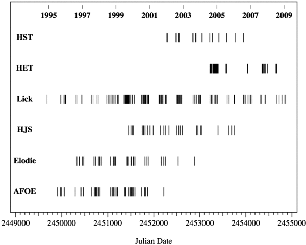
Figure 1. Times of observations of the five radial velocity sources (AFOE, Elodie, HJS, Lick, and HET) and HST—the astrometric source.
Download figure:
Standard image High-resolution imageTable 3. HET Relative Radial Velocities for υ And
| JD − 2,450,000 | RV (m s−1) | ± Error |
|---|---|---|
| 3220.855083 | 88.18 | 8.42 |
| 3221.851560 | 59.52 | 5.30 |
| 3222.857669 | 139.98 | 4.78 |
| 3227.838449 | 156.34 | 6.61 |
| 3237.839341 | 181.21 | 7.44 |
| 3240.843498 | 67.25 | 4.86 |
| 3255.800928 | 146.32 | 5.13 |
| 3257.762190 | 46.36 | 4.49 |
| 3261.755993 | 104.59 | 4.18 |
| 3263.778727 | 25.67 | 5.24 |
| 3265.771444 | 149.36 | 5.73 |
| 3286.698745 | 35.97 | 4.49 |
| 3288.669645 | 171.86 | 4.78 |
| 3293.678115 | 156.09 | 4.66 |
| 3295.673163 | 42.51 | 5.21 |
| 3297.657779 | 188.59 | 4.81 |
| 3299.884582 | 47.13 | 7.00 |
| 3302.637724 | 196.58 | 6.87 |
| 3306.852533 | 201.12 | 6.58 |
| 3310.846963 | 165.25 | 8.05 |
| 3313.852023 | 67.26 | 6.79 |
| 3315.623737 | 198.08 | 8.64 |
| 3319.825960 | 162.50 | 6.87 |
| 3321.605156 | 208.33 | 7.62 |
| 3327.587001 | 95.66 | 8.45 |
| 3330.570166 | 226.06 | 7.56 |
| 3337.561394 | 106.72 | 9.08 |
| 3340.779610 | 151.59 | 8.28 |
| 3341.763587 | 112.84 | 7.90 |
| 3342.780068 | 172.27 | 9.48 |
| 3347.779610 | 204.55 | 10.67 |
| 3358.712495 | 191.51 | 10.00 |
| 3359.717439 | 110.21 | 10.70 |
| 3360.734667 | 113.24 | 9.71 |
| 3361.741070 | 206.51 | 11.01 |
| 3365.718103 | 168.28 | 11.02 |
| 3366.705087 | 233.64 | 10.64 |
| 3369.675249 | 111.82 | 10.57 |
| 3371.691010 | 233.01 | 11.20 |
| 3377.686322 | 125.63 | 9.44 |
| 3378.662047 | 100.54 | 9.07 |
| 3379.663556 | 146.99 | 8.41 |
| 3389.638749 | 219.99 | 9.32 |
| 3392.635122 | 83.47 | 8.93 |
| 3395.621947 | 178.55 | 9.34 |
| 3396.620749 | 93.04 | 9.62 |
| 3399.620826 | 223.17 | 9.07 |
| 3568.909399 | 107.72 | 4.60 |
| 3570.908804 | 163.67 | 6.50 |
| 3575.902647 | 129.85 | 4.77 |
| 3582.896324 | 122.71 | 4.72 |
| 4034.662587 | 123.16 | 6.61 |
| 4035.646686 | 202.16 | 6.65 |
| 4035.881128 | 213.81 | 6.73 |
| 4036.888984 | 233.12 | 7.06 |
| 4037.672876 | 189.93 | 6.40 |
| 4037.866313 | 170.58 | 7.30 |
| 4038.638060 | 117.18 | 7.91 |
| 4039.624219 | 150.78 | 7.72 |
| 4039.862780 | 180.93 | 7.11 |
| 4040.627633 | 246.34 | 7.19 |
| 4040.864058 | 265.08 | 7.57 |
| 4041.628609 | 249.18 | 7.49 |
| 4352.779142 | 128.86 | 4.37 |
| 4357.752316 | 132.66 | 4.07 |
| 4357.987559 | 146.27 | 3.65 |
| 4361.742742 | 122.16 | 4.31 |
| 4368.727128 | 244.91 | 3.51 |
| 4370.738514 | 134.76 | 3.68 |
| 4377.944310 | 243.52 | 3.79 |
| 4401.640682 | 224.13 | 3.66 |
| 4422.806929 | 112.94 | 4.57 |
| 4423.564408 | 164.27 | 4.52 |
| 4467.706165 | 43.03 | 8.52 |
| 4653.940848 | 95.88 | 10.16 |
| 4659.927672 | 180.09 | 9.55 |
| 4663.922889 | 149.26 | 10.16 |
| 4669.885271 | 126.24 | 9.83 |
| 4671.894518 | 40.70 | 9.81 |
3.2. HST Astrometry Observations
FGS-1r a two-axis, white-light interferometer aboard HST was used to make the astrometric observations in position (POS) "fringe-tracking" mode. A detailed description of this instrument is found in Nelan (2007).7 Our data sets were reduced and calibrated as detailed in Benedict et al. (2007). This data set used a new improved optical field angle distortion (OFAD) calibration (McArthur et al. 2002), as yet unpublished. The astrometric data used in this research is available from the HST Program Schedule and Information Web site,8 in proposal numbers 9407, 9971, and 10103. The two-step pipeline used to reduce the raw data to the values used in this modeling is available with the latest calibration parameters from the Space Telescope Science Institute in IRAF STSDAS and in a standalone version available from one of the coauthors, the HST FGS Instrument Scientist at STScI Ed Nelan (nelan@stsci.edu).
Data are downloaded from the HST online archival retrieval system and processed through the two-stage pipeline system. The initial calibration pipeline extracts the astrometry measurements (typically 1–2 minutes of fringe position information acquired at a 40 Hz rate, which yields several thousand discrete measurements) and the median (after outlier removal), and estimates the errors. The second calibration stage applies the OFAD which is variant over time, and corrects the velocity aberration, processes the time tags, and uses the JPL Earth orbit predictor Standish (1990) to calculate the parallax factors. The methodology of the OFAD is discussed in several calibration papers (McArthur et al. 1997, 2002, 2006). Ongoing stability tests (LTSTABs) maintain this calibration. Systematics introduced by our instrument (such as intra-orbit drift and color and filter effects) and their corrections are discussed below. After 18 years of calibration, we have not uncovered additional systematics in our data which are above our detection limits. Regression analysis between Hipparcos and HST parallax measurements has shown not only good agreement between Hipparcos and HST parallaxes (with the exception of the Pleiades), but an overestimation of error of HST astrometric measurements (Benedict & McArthur 2004; Benedict et al. 2007).
Fifty-four orbits of the HST were used to make 13 epochs of astrometric observations between December of 2001 and August of 2006. Every orbit contains several observations of υ And and surrounding reference stars. The distribution of the reference stars in the υ And field is shown in the Digital Sky Survey image in Figure 2. The FGS measures the position of each star position sequentially. Each epoch contains multiple visits, alternating between the target (υ And) and the 10 reference stars, providing x(t) and y(t) positions in the HST reference frame in seconds of arc. Observations during an orbit were corrected for slow FGS intra-orbit positional drift by using an adaptable polynomial fitting routine (Benedict et al. 2007). Because υ And is a bright star (V = 4.09), a neutral density filter (F5ND) was used for observing it. For the reference stars, the F583W filter was used. The dates of observation, the epoch group of the observation, the number of measurements of υ And for each date, and the HST orientation angles are listed on Table 4. For the day of the year, letters following the day indicate more than one observation set for a single day. The HST astrometric data for υ And and its reference stars is available only online as a machine-readable table (Table 5). For the most current calibration, the data should be retrieved from the HST online archival retrieval system and processed through the two-stage pipeline system.
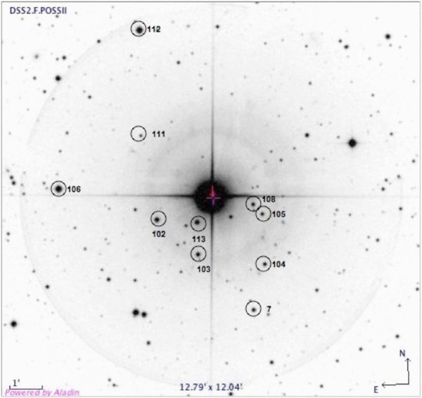
Figure 2. υ And field with astrometric reference stars marked. Reference star 113 is υ And B. The box is 15' across.
Download figure:
Standard image High-resolution imageTable 4. Dates of HSTAstrometric Observations
| Orbit | Epoch | Year | Day | Nobs | HST Roll |
|---|---|---|---|---|---|
| 1 | 1 | 2001 | 365 | 4 | 117.92 |
| 2 | 2 | 2002 | 22 | 5 | 124.90 |
| 3 | 2 | 2002 | 023A | 5 | 124.90 |
| 4 | 2 | 2002 | 023B | 5 | 124.90 |
| 5 | 2 | 2002 | 024A | 5 | 124.90 |
| 6 | 2 | 2002 | 024B | 5 | 124.90 |
| 7 | 3 | 2002 | 207 | 4 | 296.08 |
| 8 | 3 | 2002 | 209 | 4 | 296.08 |
| 9 | 3 | 2002 | 211 | 4 | 296.08 |
| 10 | 3 | 2002 | 213 | 4 | 296.08 |
| 11 | 3 | 2002 | 216 | 4 | 296.08 |
| 12 | 3 | 2002 | 219 | 4 | 296.08 |
| 13 | 4 | 2002 | 267 | 4 | 340.15 |
| 14 | 4 | 2002 | 269 | 4 | 340.15 |
| 15 | 4 | 2002 | 271 | 4 | 340.15 |
| 16 | 4 | 2002 | 274 | 4 | 340.15 |
| 17 | 4 | 2002 | 276 | 4 | 340.15 |
| 18 | 4 | 2002 | 278 | 4 | 340.15 |
| 19 | 5 | 2003 | 206 | 4 | 296.08 |
| 20 | 5 | 2003 | 208 | 4 | 296.08 |
| 21 | 5 | 2003 | 210 | 4 | 296.08 |
| 22 | 5 | 2003 | 213 | 4 | 296.08 |
| 23 | 5 | 2003 | 215 | 4 | 296.08 |
| 24 | 5 | 2003 | 217 | 4 | 296.08 |
| 25 | 6 | 2003 | 267 | 4 | 340.16 |
| 26 | 6 | 2003 | 269 | 4 | 340.16 |
| 27 | 6 | 2003 | 271 | 4 | 340.16 |
| 28 | 6 | 2003 | 274 | 4 | 340.16 |
| 29 | 6 | 2003 | 277 | 4 | 340.16 |
| 30 | 6 | 2003 | 279 | 4 | 340.16 |
| 31 | 7 | 2004 | 41 | 5 | 124.90 |
| 32 | 7 | 2004 | 43 | 5 | 124.90 |
| 33 | 7 | 2004 | 45 | 4 | 124.90 |
| 34 | 7 | 2004 | 47 | 5 | 124.90 |
| 35 | 7 | 2004 | 49 | 5 | 124.90 |
| 36 | 7 | 2004 | 51 | 5 | 124.90 |
| 37 | 8 | 2004 | 208 | 4 | 296.08 |
| 38 | 8 | 2004 | 211 | 4 | 296.08 |
| 39 | 8 | 2004 | 214 | 4 | 296.08 |
| 40 | 9 | 2004 | 268 | 4 | 340.16 |
| 41 | 9 | 2004 | 270 | 4 | 340.16 |
| 42 | 9 | 2004 | 272 | 4 | 340.16 |
| 43 | 10 | 2005 | 42 | 5 | 124.90 |
| 44 | 10 | 2005 | 45 | 5 | 124.90 |
| 45 | 10 | 2005 | 48 | 5 | 124.90 |
| 46 | 11 | 2005 | 210 | 4 | 296.08 |
| 47 | 11 | 2005 | 212 | 4 | 296.08 |
| 48 | 11 | 2005 | 214 | 4 | 296.08 |
| 49 | 12 | 2006 | 38 | 5 | 123.90 |
| 50 | 12 | 2006 | 40 | 5 | 123.90 |
| 51 | 12 | 2006 | 42 | 5 | 123.90 |
| 52 | 13 | 2006 | 211 | 4 | 296.08 |
| 53 | 13 | 2006 | 213 | 4 | 296.08 |
| 54 | 13 | 2006 | 216 | 4 | 296.08 |
Download table as: ASCIITypeset image
Table 5. HST Astrometric Data for υ And A and B and Reference Starsa
| Set | Obs ID | Star | rollV3 | Filter | Xmad | Ymad | Xvaofadapj2d | Yvaofadapj2d |
|---|---|---|---|---|---|---|---|---|
| 1 | F6KG0101M | 1 | 117.9157 | F5ND | 0.0042 | 0.00189 | −0.769 | 760.218 |
| 1 | F6KG0102M | 106 | 117.9157 | F583W | 0.0048 | 0.00251 | 260.391 | 649.097 |
| 1 | F6KG0103M | 102 | 117.9157 | F583W | 0.0041 | 0.00211 | 74.206 | 679.250 |
| 1 | F6KG0104M | 103 | 117.9157 | F583W | 0.0047 | 0.00305 | −21.014 | 656.519 |
| 1 | F6KG0105M | 104 | 117.9157 | F583W | 0.0040 | 0.00268 | −138.289 | 694.918 |
| 1 | F6KG0106M | 105 | 117.9157 | F583W | 0.0038 | 0.00199 | −93.484 | 774.678 |
Only a portion of this table is shown here to demonstrate its form and content. A machine-readable version of the full table is available.
Download table as: DataTypeset image
3.3. Spectrophotometric Parallaxes for the Reference Stars
Because the parallax determined for υ And is measured with respect to reference frame stars which have their own parallaxes, we must either apply a statistically derived correction from relative to absolute parallax (van Altena et al. 1995, Yale Parallax Catalog, hereafter YPC95), or estimate the absolute parallaxes of the reference frame stars. In principle, the colors, spectral type, and luminosity class of a star can be used to estimate the absolute magnitude, MV, and V-band absorption, AV. The absolute parallax is then simply,

3.3.1. Reference Star Photometry
Our bandpasses for reference star photometry include V (from FGS-1r) and JHK from 2MASS.9 The JHK values have been transformed to the Bessell & Brett (1988) system using the transformations provided in Carpenter (2001). Table 6 lists VJHK photometry for the target and reference stars indicated in Figures 2. Figure 3 contains a (J − K) versus (V − K) color–color diagram with reference stars and υ And labeled. Schlegel et al.(1998) find an upper limit AV∼ 0.3 toward υ And. In the following, we adopt 〈AV〉 = 0.0 for all but ref-105, ref-108, and ref-112. We increase the error on those reference star distance moduli by 1 mag to account for absorption uncertainty.
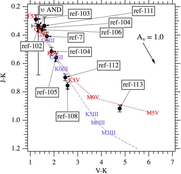
Figure 3. (J − K) vs. (V − K) color–color diagram for stars identified in Table 6. The dashed line is the locus of dwarf (luminosity class V) stars of various spectral types; the dot-dashed line is for giants (luminosity class III). The reddening vector indicates AV = 1.0 for the plotted color systems. Along this line of sight maximum extinction is AV ∼ 0.3 (Schlegel et al. 1998).
Download figure:
Standard image High-resolution imageTable 6. V and Near-IR Photometry of υ And A and B and Astrometric Reference Stars
| ID | V | K | (J − H) | (J − K) | (V − K) |
|---|---|---|---|---|---|
| υ And A | 4.24 ± 0.01 | 2.90 ± 0.27 | 0.27 ± 0.28 | 0.34 ± 0.35 | 1.34 ± 0.27 |
| 7 | 14.22 ± 0.01 | 12.52 ± 0.02 | 0.33 ± 0.03 | 0.41 ± 0.03 | 1.70 ± 0.03 |
| 102 | 13.11 ± 0.01 | 11.77 ± 0.02 | 0.33 ± 0.03 | 0.35 ± 0.03 | 1.35 ± 0.02 |
| 103 | 13.77 ± 0.01 | 12.53 ± 0.03 | 0.28 ± 0.03 | 0.29 ± 0.03 | 1.24 ± 0.03 |
| 104 | 14.51 ± 0.01 | 12.62 ± 0.02 | 0.38 ± 0.03 | 0.52 ± 0.03 | 1.89 ± 0.02 |
| 105 | 14.82 ± 0.01 | 12.73 ± 0.02 | 0.47 ± 0.03 | 0.56 ± 0.03 | 2.09 ± 0.03 |
| 106 | 11.41 ± 0.01 | 9.92 ± 0.02 | 0.35 ± 0.03 | 0.36 ± 0.02 | 1.49 ± 0.02 |
| 108 | 14.62 ± 0.01 | 12.05 ± 0.02 | 0.67 ± 0.02 | 0.76 ± 0.02 | 2.57 ± 0.02 |
| 111 | 15.82 ± 0.01 | 14.23 ± 0.06 | 0.34 ± 0.04 | 0.34 ± 0.06 | 1.59 ± 0.06 |
| 112 | 11.78 ± 0.01 | 9.31 ± 0.02 | 0.60 ± 0.02 | 0.70 ± 0.02 | 2.48 ± 0.02 |
| υ And B | 13.86 ± 0.01 | 8.55 ± 0.02 | 0.62 ± 0.04 | 0.92 ± 0.02 | 4.77 ± 0.02 |
Download table as: ASCIITypeset image
The derived absolute magnitudes are critically dependent on the assumed stellar luminosity, a parameter impossible to obtain for all but the latest type stars using only Figure 3. To confirm the luminosity classes, we obtain NOMAD proper motions (Zacharias et al. 2005) for a one-degree-square field centered on υ And, and then iteratively employ the technique of reduced proper motion (Yong & Lambert 2003; Gould & Morgan 2003) to discriminate between giants and dwarfs. The end result of this process is contained in Figure 4.
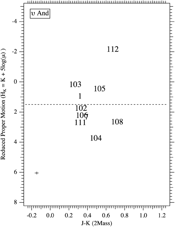
Figure 4. Reduced proper motion diagram for 3480 stars in a 1° field centered on υ And. Star identifications are in Table 6. For a given spectral type, giants and sub-giants have more negative HK values and are redder than dwarfs in (J − K). HK values are derived from "Final" proper motions in Table 8. The small cross at the lower left represents a typical (J − K) error of 0.04 mag and HK error of 0.17 mag. The horizontal dashed line is a giant-dwarf demarcation derived from a statistical analysis of the Tycho input catalog (D. Ciardi 2004, private communication). Ref-112, -108, and -105 are likely luminosity class III.
Download figure:
Standard image High-resolution image3.3.2. Estimated Reference Frame Absolute Parallaxes
We derive absolute parallaxes using our estimated spectral types and luminosity class and MV values from Cox (2000). Our adopted input errors for distance moduli, (m − M)0, are 0.4 mag for all reference stars (except ref-105, ref-108, and ref-112, as discussed above). Contributions to the error are a small but undetermined AV and errors in MV due to uncertainties in color to spectral type mapping. All reference star absolute parallax estimates are listed in Table 7. Individually, no reference star absolute parallax is better determined than  = 18%. The average input absolute parallax for the reference frame is 〈πabs〉 = 1.44 mas, a quantity known to ∼5% (standard deviation of the mean of nine reference stars). We compare this to the correction to absolute parallax discussed and presented in YPC95 (Section 3.2, Figure 3). Entering YPC95, Figure 3, with the Galactic latitude of υ And, b = −21°, and average magnitude for the reference frame, 〈Vref〉 = 13.53, we obtain a correction to absolute parallax of 1.5 mas, in good agreement with our average input absolute parallaxes for the reference frame. Rather than apply a model-dependent correction to absolute parallax, we introduce our spectrophotometrically estimated reference star parallaxes into our reduction model as observations with error.
Table 7. Astrometric Reference Star Adopted Spectrophotometric Parallaxes
| ID | Sp. T.a | V | MV | m−M | πabs (mas) |
|---|---|---|---|---|---|
| 7 | G5V | 14.22 | 5.1 | 9.12 ± 0.4 | 1.5 ± 0.3 |
| 102 | G5V | 13.11 | 4.4 | 8.71 ± 0.4 | 2.5 ± 0.3 |
| 103 | F7V | 13.77 | 3.9 | 9.91 ± 0.4 | 1.0 ± 0.2 |
| 104 | G5V | 14.51 | 5.9 | 8.61 ± 0.4 | 1.3 ± 0.3 |
| 105 | G5III | 14.82 | 0.9 | 13.92 ± 1.0 | 0.2 ± 0.1 |
| 106 | G4V | 11.41 | 5.0 | 6.45 ± 0.4 | 5.1 ± 0.9 |
| 108 | K2IV | 14.62 | 3.5 | 11.13 ± 1.0 | 0.6 ± 0.3 |
| 111 | G3V | 15.82 | 4.8 | 11 ± 0.4 | 0.6 ± 0.1 |
| 112 | K1III | 11.78 | 0.6 | 13.68 ± 1.0 | 0.2 ± 0.1 |
Note. aSpectral types and luminosity class estimated from colors and reduced proper motion diagram.
Download table as: ASCIITypeset image
3.3.3. Estimated Reference Frame Proper Motions
Typically, we use proper motion values from NOMAD or its predecessor UCAC2 (Zacharias et al. 2005) as observations with error in the model. We have found these catalogs to be excellent sources of proper motion information and integral to all of our results. In this case, we found in our modeling of the reference frame alone differences between the NOMAD values and our astrometric data in three of the reference stars (7, 104, and 108), while the other five reference stars that had values in the NOMAD catalog were in relative agreement. We iteratively modeled the reference frame alone, to derive more realistic values for the proper motions. Our HST observations spanned about five years, with on average 90 observations per reference star, while the conflicting values in the NOMAD catalog were high error results based upon four or less observations. The NOMAD proper motions, the reference frame derived values and our final model values can be seen in Table 8.
Table 8. Astrometric Reference Star Proper Motions
| ID | Input (NOMAD) | Reference Frame Derived (HST) | Final (HST) | |||
|---|---|---|---|---|---|---|
| μαa | μδa | μα | μδ | μα | μδ | |
| 7 | −2.8 ± 5.9 | −9.0 ± 5.9 | −1.41 ± 0.93 | −0.54 ± 0.91 | −1.31 ± 0.09 | −0.45 ± 0.10 |
| 102 | −9.6 ± 2.3 | −3.5 ± 2.1 | −10.02 ± 0.35 | −0.61 ± 0.38 | −10.08 ± 0.07 | −0.59 ± 0.06 |
| 103 | −2.2 ± 9.0 | −2.7 ± 9.0 | −4.18 ± 0.51 | 1.77 ± 0.52 | −4.17 ± 0.1 | 1.74 ± 01 |
| 104 | −0.2 ± 5.9 | −17.3 ± 5.8 | −1.06 ± 0.60 | −8.49 ± 0.62 | −1.03 ± 0.11 | −8.50 ± 0.1 |
| 105 | −0.4 ± 9.0 | −3.6 ± 9.0 | −0.86 ± 0.57 | −2.70 ± 0.65 | −0.88 ±0.15 | −2.72 ± 0.14 |
| 106 | −1.4 ± 0.6 | −29.7 ± 0.6 | −0.80 ± 0.62 | −29.18 ± 0.63 | −0.71 ± 0.09 | −29.21 ± 0.08 |
| 108 | −1.3 ± 9.0 | −13.6 ± 9.0 | −3.91 ± 0.37 | −0.76 ± 0.43 | −3.90 ± 0.08 | −0.76 ± 0.08 |
| 112 | −4.9 ± 1.0 | −1.9 ± 0.6 | −4.90 ± 1.00 | −1.90 ± 0.60 | −4.86 ± 0.24 | −1.90 ± 0.18 |
Note. aμα and μδ are relative motions in milliseconds of arc yr−1.
Download table as: ASCIITypeset image
3.4. Astrometric Model
The υ And reference frame contained a very generous field of 10 (nine usable) reference stars plus υ And B. With the positions (x', y') measured by FGS-1r, we build an overlapping plate model that accounts for scale, rotation, and offset relative to an arbitrarily adopted constraint or "master" plate. The astrometric model also accounts for the time-dependent movements of each star, given by the absolute parallax πabs and the proper motion components, μα and μδ, and the corrections for the cross-filter and lateral color positional shifts. Therefore, the model is given by the standard coordinates ξ and η in these equations of condition:


where x and y are the measured coordinates from HST; lcx and lcy are the lateral color corrections, and B − V are the B − V colors of each star; ΔXFx and ΔXFy are the cross-filter corrections in x and y, applied only to the observations of υ And. A and B are scale and rotation plate constants, C and F are offsets, μα and μδ are proper motions, Δt is the epoch difference from the mean epoch, Pα and Pδ are parallax factors, and π is the parallax. We obtain the parallax factors from a JPL Earth orbit predictor Standish (1990), upgraded to version DE405. In order to find a global solution, we used a program written in the GAUSSFIT language (Jefferys et al. 1988). ORBIT is a function using Thiele–Innes constants (Heintz 1978) of the traditional astrometric and RV orbital elements. Table 9 shows the resulting astrometric catalog from the combined orbital modeling.
Table 9. Astrometric Catalog
| Star | Mag | R.A.a | Decl.a | ξb | σξ | η | ση |
|---|---|---|---|---|---|---|---|
| V | (deg) | (deg) | (arcsec) | (arcsec) | (arcsec) | (arcsec) | |
| υ And A | 4.13 | 24.19904 | 41.405320 | 55.65925 | 0.00010 | 707.29045 | 0.00009 |
| 7 | 14.16 | 24.17446 | 41.348200 | 271.08537 | 0.00014 | 713.27128 | 0.00012 |
| 102 | 13.07 | 24.23800 | 41.395040 | 53.40737 | 0.00011 | 817.61938 | 0.00010 |
| 103 | 13.71 | 24.21070 | 41.377100 | 139.38278 | 0.00016 | 770.81501 | 0.00014 |
| 104 | 14.45 | 24.16658 | 41.371350 | 200.87260 | 0.00019 | 663.82158 | 0.00017 |
| 105 | 14.78 | 24.16658 | 41.396760 | 114.19421 | 0.00026 | 634.51811 | 0.00025 |
| 106 | 11.38 | 24.30410 | 41.411960 | −64.76309 | 0.00013 | 964.63260 | 0.00013 |
| 108 | 14.61 | 24.17229 | 41.401860 | 92.04375 | 0.00015 | 643.65448 | 0.00013 |
| 112 | 11.75 | 24.24677 | 41.491300 | −280.15568 | 0.00024 | 720.63553 | 0.00020 |
| υ And B | 13.84 | 24.20987 | 41.392100 | 90.37398 | 0.00030 | 750.71189 | 0.00018 |
Notes.
aPredicted coordinates for equinox J2000.0.
bRelative coordinates in the reference frame of the constrained plate (set 29, with roll = 3401552).
Download table as: ASCIITypeset image
There are additional equations of condition relating an initial value (an observation with associated error) and final parameter value. For the reference stars, there are equations in the model for proper motion and spectrophotometric parallax. For the target star (υ And), we add equations for cross filter. Both target and reference stars have equations for lateral color parameters. The roll of the plates also has a condition equation. Through these additional equations of condition, the χ2 minimization process is allowed to adjust parameter values by amounts constrained by the input errors. In this quasi-Bayesian approach, prior knowledge is input as an observation with associated error, not as a hardwired quantity known to infinite precision. For υ And A and B, no priors were used for parallax or proper motion. These values and the orbital parameters were determined independently without bias.
3.4.1. Astrometric Reference Frame Residual Assessment
Before the target star, υ And, is modeled simultaneously with the reference frame, the reference frame is independently modeled many times to assess the which plate model is appropriate, prior knowledge of spectrophotometric parallaxes, catalog proper motions, and stability as a reference star. Poor fits of the reference frame can lead to reassessment of the spectrophotometric parallaxes, derivation of independent proper motion estimates, and removal of "bad" reference stars. In this case, reference Star 111 was not used in the modeling because this 15.82 mag star either had false locks in the interferometer (which can occur with faint stars), or it is a double star.
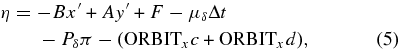
The OFAD calibration (McArthur et al. 2002) reduces the as-built HST telescope and FGS-1r distortions with amplitude of more than 1 arcsec to below 2 mas over much of the FGS-1r field of regard. From histograms of the υ And field astrometric residuals shown in Figure 5, we conclude that we have obtained satisfactory correction. The resulting reference frame "catalog" in ξ and η standard coordinates was determined with average position errors 〈σξ〉 = 0.17 and 〈ση〉 = 0.16 mas.
Figure 5. Histograms of the astrometric frame residuals of the fit.
Download figure:
Standard image High-resolution imageTo determine whether there might be unmodeled, but possibly correctable, systematic instrumental effects at the 1 mas level, we plotted reference frame x and y residuals against a number of spacecraft, instrumental, and astronomical parameters. These included x, y position within our total field of view, radial distance from the field-of-view center, reference star V magnitude and B − V color, and epoch of observation. We saw no obvious trends.
3.5. RV Model
We model the radial ( ) component of the stellar orbital movement around the barycenter of the system. This is given by the projection of a Keplerian orbital velocity to observer's line of sight plus a constant velocity offset.

where e is eccentricity, ω is the longitude of periastron, K1 is the semi-amplitude of the RV signal, E is the eccentric anomaly from Kepler's equation, and γ is the constant velocity offset. We model three planetary orbits, one slope (indicating an additional long-period companion) and five γ's, one for each data set. Additionally, a systematic slope found only in the AFOE data was modeled.
3.6. Combined Orbital Model
We use an unperturbed Keplerian orbit with linear combination of Keplerian orbits, which is an acceptable first-order approximation of the orbital elements. Our long-term stability tests perform a full computation of perturbed orbits, which is considered in detail in Section 5. Additionally, we constrain a relationship between the astrometry and the RV through this equation (Pourbaix & Jorissen 2000):
where quantities only derivable from the astrometry (parallax, πabs, primary perturbation orbit size, α, and inclination, i) are on the left, and quantities derivable from both (the period, P, and eccentricity, e), or radial velocities only (the RV amplitude of the primary, K), are on the right.
We investigated the use of alternative orbital modeling software (Systemic10) that considered perturbations, but found that they included assumptions, such as an inclination of 90°and coplanarity (S. Meschiari 2009, private communication), that would have presented a less realistic interpretation of our data. We did create an orbital model which included N-body perturbations, which is discussed in Section 4.2.1.
4. RESULTS
4.1. HST Parallax and Proper Motions of υ And and υ And B
Serendipitously, one of our reference stars (ref-113) was υ And B (= 2MASS J01365042+412332). This gave us the opportunity to assess its status as the stellar companion to υ And. υ And B was first announced in early 2002 (Lowrance et al. 2002) as a distant stellar companion at an apparent projected separation of ∼750 AU. Its association was determined by the calculation of a similar proper motion from the POSS I and POSS II digitized images. Later in 2002, an attempt was made to detect a binary companion to stars with planets including υ And using high-resolution and wide-field imaging with Keck and Lick (Patience et al. 2002). The conclusion of this study was that because there should have been a detection of υ And B, but there was not, that it was a background object. In 2004, it was included in the study of stellar multiples of Eggenberger et al. (2004). In 2006, Raghavan et al. (2006) proposed a projected separation of 702 AU between components A and B, and noted that they were not gravitationally bound.
We find a parallax of 73.71 ± 0.10 mas for υ And and 73.45 ± 0.44 mas for υ And B (shown along with proper motions in Table 10, including the HIPPARCOS values for comparison). This is a separation in parallax between υ And and υ And B of 0.26 mas which is about 0.048 parsecs or ∼9900 AU. The previous estimates of separations are within our errors which support separations less than ∼30,000 AU. The parallax and proper motions uncertainties of υ And B are higher than normal because a significant portion of the observations could not be used because diffraction spikes from υ And contaminated the data. HST proper motions are relative to the reference frame that we observed.
Table 10. Parallax and Proper Motions of υ And A and B
| ID | Parallax | μx | μy |
|---|---|---|---|
| HST υ And A | 73.71 ± 0.10 | −173.22 ± 0.06 | −381.80 ± 0.05 |
| HST υ And B | 73.45 ± 0.44 | −172.77 ± 0.27 | −382.45 ± 0.38 |
| HIP υ And A | 74.25 ± 0.72 | −172.57 ± 0.52 | −381.03 ± 0.45 |
Download table as: ASCIITypeset image
4.2. Orbital Solution
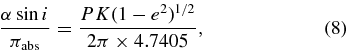
The updated orbital parameters of υ And presented in Butler et al. (2006) were based upon 268 observations from Lick Observatory. For our combined orbital solution, we had 974 RV observations, including the new data from the HET. We ran periodograms on the residuals from these fits: (1) only γ's fitted, (2) γ's and planet b fitted, (3) γ's and planets b and c fitted, and (4) γ's and planets b, c, and d fitted. We looked for evidence of additional planetary periodic signals in these periodograms (see Figure 6). In the periodogram of the residuals to a Keplerian model that contains the planet b, c, and d, we see a weak signal at around one month and a presumed systematic signal at around 180 days that originated in the Lick data, as mentioned in Butler et al. (1999). We found no indications of additional planetary objects from these periodograms. We also examined the residuals in phase space and time plots and did note a large slope (∼35 ms-1) spanning the ∼ 6.3 year AFOE data set. After applying a linear correction to this data, the residuals of the AFOE velocities decreased by 30%.
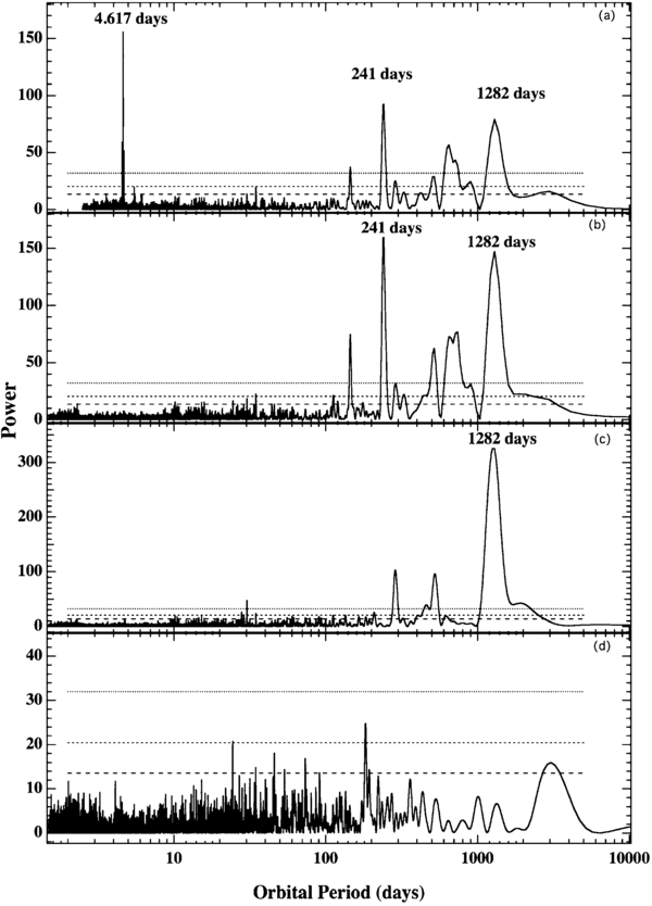
Figure 6. Periodogram of the radial velocity data of υ Andromedae from five sources. (a) Shows peaks for planets b (4.617 days), c (241 days), and d (1282 days). The false alarm probability of the peak at 4.617 days is 1.186e−64. (b) Shows the periodogram of the residuals of a Keplerian model that contains planet b; planets c (period 241 days) and planet d (1282 days) can still be seen. The false alarm probability of the peak at 241 days is 2.775e−68. (c) Shows the periodogram of the residuals of a Keplerian model that contains the planets b and c; planet d (1282 days) can still be seen. The false alarm probability of the peak at 1269 days is 1.057e−139. (d) Shows periodogram of the residuals to a Keplerian model that contains the planet b (period 4.617 days), planet c (241 days), and planet d (1282 days). The periodogram shows a systematic from the Lick data at 180 days. The dotted lines show the significance levels of the power in each plot, from the top: 1.0e−10, 1.0e−5, and 1.0e−2.
Download figure:
Standard image High-resolution imageIf we find no additional periodic signals to model from the periodograms or inspection of the residuals, we add a slope to the model to test for a longer period planet. Table 11 shows the χ2, degrees of freedom (dof), and rms of the various υ And independent RV planet modeling. We find a significant χ2 improvement (from 745 down to 606) for the additional 1 degree of freedom, which we interpret as evidence of this long-period object. The amplitude of the trend is approximately 2.5 ms-1 over the 14 year data set.
Table 11. υ And RV Modeling
| Model | χ2 | dof | rms (m s−1) |
|---|---|---|---|
| No planetsa | 30936 | 828 | 72.39 |
| b | 18100 | 823 | 54.67 |
| b + c | 9206 | 818 | 40.03 |
| b + c + d | 745 | 813 | 11.60 |
| b + c + d + slope | 606 | 812 | 10.66 |
Note. aSolve for γ offsets only.
Download table as: ASCIITypeset image
From previous work (Benedict et al. 2002; Bean et al. 2007; Martioli et al. 2010) and exploratory analysis, we have confidence in conservatively detecting astrometric signals down to around 0.25 mas. Of the three well-determined planets around υ And, only planet d would have an astrometric signal that would be detectable by the HST FGS at all inclinations (see Figure 7 noting that α is the half-amplitude of the astrometric signal). Planet b could be detected if its inclination was less than 12, planet c if its inclination was less than ∼44° and planet d could be detected at any inclination.
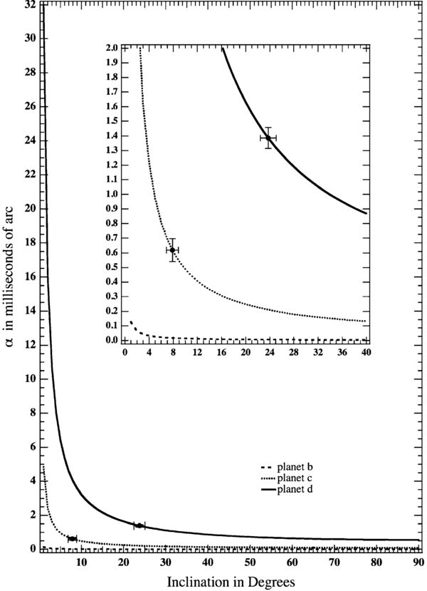
Figure 7. Astrometric α, perturbation, against inclination for the three planets as calculated from Equation (8). The HST determined α's for υ And c and d are shown with error bars on the plots. The inset zooms in on components c and d.
Download figure:
Standard image High-resolution imageSimultaneous astrometric and RV modeling was carried out using GaussFit. (For a review of the use of GaussFit for problems of linear regression with errors in both variables and the errors it produces see Murtagh 1990.) Astrometric modeling of the target and reference frame consisted of scale, lateral color, cross filter, proper motion, parallax, and the astrometric orbital elements of either planet d alone or planets c and d or planets b, c, and d, and was carried out as detailed in Section 3.4, with RV modeling of a slope and planets b, c, and d. Our modeling program GaussFit allows us to set a tolerance that prevents a solution being found in a shallow minima. That setting combined with the simultaneous modeling of free parameters (no parameters are held as constants) minimizes the chance of false detection.
Our attempt at the simultaneous astrometric modeling of planets b, c, and d failed. With all parameters free, the program iterated endlessly rather than settling on a false detection, indicating that there was no detectable astrometric signal for planet b. However, when we only modeled the astrometric signals of planets c and d with the same method, we detected the astrometric signal of planets c and d. The modeling of the orbital elements determined simultaneously with GaussFit, using robust estimation, including the astrometric signals of planets c and d had improved χ2 and lowered residuals over the same model which did not include the astrometric orbit of planets c and d. In Table 12, we show the χ2 improvement after the cumulative addition of the astrometric modeling components. These are stepwise astrometric models with the RV elements as constants for illustrative purposes, not the simultaneous model of our solution. The final addition of the orbital elements includes the six astrometric elements of planets c and d, with the other orbital elements input as constants from our simultaneous solution. The dof in this modeling include not only the astrometric data and the parameters solved for but also the constraint equations (to control the scale of the master plate and for Pourbaix's relation) and the a priori Bayesian input data related to the proper motions and parallax of the reference frame and the lateral color and cross-filter instrument calibrations.
Table 12. υ And Astrometric Modeling
| Cumulative Model | χ2 | dof |
|---|---|---|
| Catalog positiona | 230703219979 | 1956 |
| + scaleb | 6989776 | 1638 |
| + proper motion | 44974 | 1634 |
| + parallaxc | 392 | 1630 |
| + planets | 360 | 1626 |
Notes. aSolve for ξ and η only. bIncludes rotation. cIncludes lateral color and cross-filter corrections.
Download table as: ASCIITypeset image
The χ2 of 360 for 1624 dof indicates that the astrometric data has errors that are overestimated as we have verified in comparisons with Hipparcos data (see Section 3.2). The HST astrometric error estimation is based upon complex statistical examination of the raw data, and we have chosen to continue to use these usually overestimated errors because we are not able to assign the overestimation to a particular component of the complex error estimation process. The orbital elements from this solution are shown in Table 13 along with the derived elements. Because of the overestimation of the astrometric data input errors, the actual errors of the astrometric parameters are most likely smaller than listed in the table.
Table 13. υ Andromedae A: Orbital Parameters and Masses.
| Parameter | υ And b | υ And c | υ And d |
|---|---|---|---|
| RV | |||
| K (m s−1) | 70.505 ± 0.368 | 53.480 ± 0.409 | 67.740 ± 0.461 |
| HET γ (m s−1) | 130.997 ± 0.074 | ||
| HJS γ (m s−1) | −14.362 ± 1.287 | ||
| Lick γ (m s−1) | −0.909 ± 1.850 | ||
| AFOE γ (m s−1) | 729.20 ± 5.030 | ||
| Elodie γ (m s−1) | −9.407 ± 1.598 | ||
| Astrometry | |||
| α (mas) | 0.619 ± 0.078 | 1.385 ± 0.072 | |
| i (deg) | 7.868 ± 1.003 | 23.758 ± 1.316 | |
| Ω (deg) | 236.853 ± 7.528 | 4.073 ± 3.301 | |
| Astrometry and RV | |||
| P (days) | 4.617111 ± 0.000014 | 240.9402 ± 0.047 | 1281.507 ± 1.055 |
| Ta (days) | 50034.053 ± 0.328 | 49922.532 ± 1.17 | 50059.382 ± 3.495 |
| e | 0.012 ± 0.005 | 0.245 ± 0.006 | 0.316 ± 0.006 |
| ω (deg) | 44.106 ± 25.561 | 247.659 ± 1.76 | 252.991 ± 1.311 |
| Derivedb | |||
| a (AU) | 0.0594 ± 0.0003 | 0.829 ± 0.043 | 2.53 ± 0.014 |
| Mass func (M☉) | 1.676e−10 ± 2.6e−12 | 3.48e−09 ± 6.2e−11 | 3.5191e−08 ± 5.2e−10 |
| Msin i(MJ)c | 0.69 ± 0.016 | 1.96 ± 0.05 | 4.33 ± 0.11 |
| M(MJ) | 13.98+2.3−5.3 | 10.25+0.7−3.3 | |
| Planets c and d | |||
| Mutual i (Φ) (deg) | 29.917 ± 1 | ||
Notes. aT = T − 2400000.0. bAn υ And mass of 1.31 ± 0.02 M☉ (Takeda et al. 2007) was used in these calculations. cThe quantity referred to in radial velocity studies as mass, but actually is minimum mass.
Download table as: ASCIITypeset image
We find the inclination of planet c to be 787 ± 10 and the inclination planet d to be 2376 ± 13. These values are shown in Figure 7 with error bars. The measured ascending nodes are Ωc= 236853 ± 75 and Ωd= 407 ± 33. These inclinations and ascending nodes permit a determination of the mutual inclination (Φ) of components c and d of the υ And system. Using Equation (9) (Kopal 1959):

we find the mutual inclination of υ And c and d to be 299 ± 10. The mutual inclination of the orbits of components c and d are shown schematically in Figure 8. (The error on Φ was determined by recalculating Equation (9) with inclination and ascending node values at ±1 − σ extrema and comparing the resulting Φ values.) These are measurements, not quantities derived from dynamical stability analyses. The astrometric motions of planets υ And c and d against time are shown in Figure 9, while they are shown on the sky in Figure 10. The astrometric data shown in these plots (the dark filled circles) are normal points made from the υ And residuals to an astrometric fit of the target and reference frame stars of scale, lateral color, cross filter, parallax, and proper motion of multiple observations (light open circles) at each epoch.

Figure 8. Left: orbits of υ And c and d on the sky. Darker segments of the orbits indicate out of plane, lighter behind plane of sky. Trace size is proportional to the masses of the companions. Right: perspective view of the orbits of components c and d projected on orthogonal axes.
Download figure:
Standard image High-resolution image
Figure 9. Astrometric reflex motion of υ And due to υ And c and d against time is shown. The astrometric orbit is shown by the dark line. Dark filled circles are normal points made from the υ And residuals to an astrometric fit of the target and reference frame stars of scale, lateral color, cross filter, parallax, and proper motion of multiple observations (light open circles) at each epoch. Normal point size is proportional to the number of individual measurements that formed the normal point. Error bars represent the one-sigma of the normal position. Many error bars are smaller than the symbols.
Download figure:
Standard image High-resolution image
Figure 10. Astrometric reflex motion of υ And due to υ And c and d. The astrometric orbit is shown by the dark line. Open circles show times of observations, dark filled circles are normal points made from the υ And residuals to an astrometric fit of the target and reference frame stars of scale, lateral color, cross filter, parallax, and proper motion of multiple observations (light open circles) at each epoch. Normal point size is proportional to the number of individual measurements that formed the normal point. Solid line shows the combined astrometric motion of υ And c and d from the elements in Table 13.
Download figure:
Standard image High-resolution imageFor calculations of the masses, we use an M☉ of 1.31+0.02−0.01 for υ And, which is a Bayesian-derived determination by Takeda et al. (2007), who note that though there is a probability (which is low) of the star being older and lower mass, they conclude that isochrone analyses favors the younger main-sequence model instead of the older turnoff or post-main-sequence models. We then find a minimum mass for planet b of 0.69 ± 0.016 MJUP and actual masses for planet c of 13.98+2.3−5.3 MJUP and planet d of 10.25+0.7−3.3 MJUP. The actual masses were derived from the HST astrometrically measured α's of planet c (0.619 ± 0.078) and planet d (1.385 ± 0.072). The probable actual mass range of planet b suggested by dynamical analysis is discussed in Section 5.
Figure 11 shows the RV of companions b, c, and d (with the other component velocities removed) plotted against orbital phase. The γ adjusted velocities with the combined orbital fit of the five RV data sources are shown in the top panel of Figure 12 and the velocity residuals are shown in the lower panel. Table 14 shows the number of observations and rms of the five RV data sources with an average rms of 10.66. The histogram in Figure 13 shows the Gaussian distribution of the RV residuals of the combined orbital model which include residuals from five different sources spanning 14 years. Figure 14 shows the distribution of the HET residuals alone.
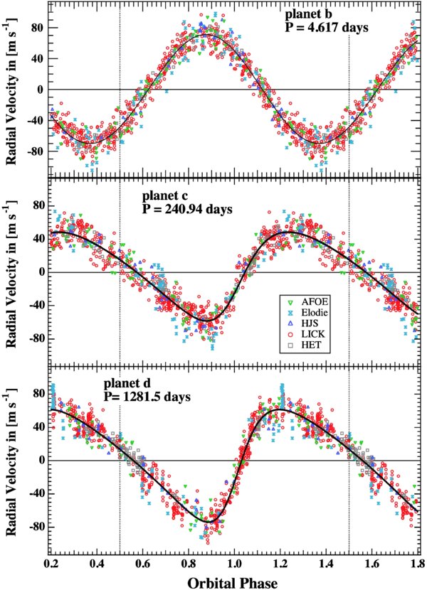
Figure 11. Residual velocities vs. orbital phase for each planet after the subtraction of the signal produced by the two other planets plus a linear trend. The orbital parameters were established with a simultaneous three-planet plus linear trend Keplerian fit to all Doppler measurements combined with HST astrometry. The solid line shows the Keplerian curve of the planet alone.
Download figure:
Standard image High-resolution image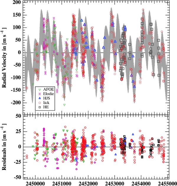
Figure 12. Radial velocities vs. time from five sources. The orbital parameters were established with a simultaneous three-planet plus linear trend Keplerian fit to all Doppler measurements combined with HST astrometry. The solid gray line shows the combined orbital fit which includes planets b, c, and d plus a linear trend (f). The lower panel shows the residuals to the fit.
Download figure:
Standard image High-resolution image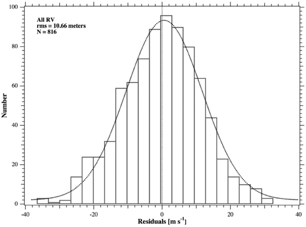
Figure 13. Histogram of the RV residuals of the simultaneous three-planet plus linear trend Keplerian fit to all Doppler measurements combined with HST astrometry.
Download figure:
Standard image High-resolution image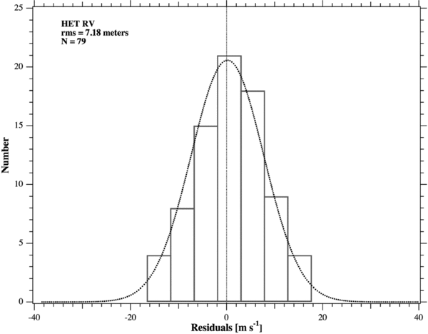
Figure 14. Histogram of the HET RV residuals of the simultaneous three-planet plus linear trend Keplerian t to all Doppler measurements combined with HST astrometry.
Download figure:
Standard image High-resolution imageTable 14. Radial Velocity Data Sets
| Data Set | Coverage | Number of Observations | rms (m s−1) |
|---|---|---|---|
| AFOE | 1995 Jul–2000 Nov | 71 | 11.84 |
| Lick | 1995 Sep–2009 Feb | 561 | 11.17 |
| Elodie | 1996 Aug–2003 Sep | 68 | 17.5 |
| McDonald HJS | 1999 Oct–2006 Jan | 37 | 10.33 |
| McDonald HETa | 2004 Aug–2008 Jul | 237 | 7.18 |
| Total | 974 | 10.66 | |
Note. aThree observations per night are combined in a single normal point.
Download table as: ASCIITypeset image
4.2.1. Orbital Solution using N-body Integrations
In addition to the above simultaneous Keplerian model orbital solution, we also performed an orbital solution using N-body integration. We used the Mercury code (Chambers 1999) with the RADAU integrator (Everhart 1985) for the integration of the equations of motion in our model. All bodies were considered not as point masses, but planets with actual mass (non-zero radii). This is a preliminary modeling process which does not include all relativistic effects, but disk loses the difference in solutions when you include the planet–planet interaction and indirect forces. The orbital elements determined with the method are listed in Table 15. Using this method, we find the mutual inclination of υ And c and d to be 309, which is within the errors to the 299 found with the simple Keplerian model. In Figure 15, we show the Keplerian and perturbed orbital solutions plotted together. While the small microarcsecond difference affects our determination of mutual inclination within the errors, it is clear that with data from the Space Interferometry Mission (SIM), orbital modeling will have to enter a new level of precision, and current methods of determining gravitational and relativistic effects will have to be enhanced.
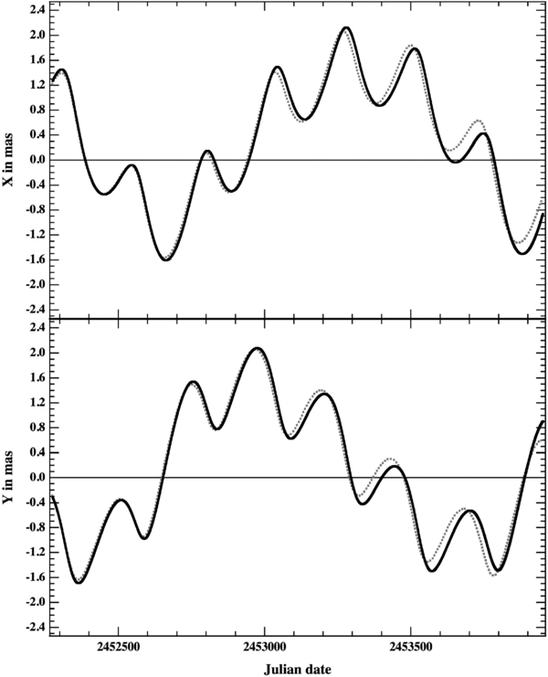
Figure 15. Astrometric reflex motion of υ And due to υ And c and d against time. The Keplerian orbit is shown as a solid dark line, the N-body integrated orbit as a gray dotted line.
Download figure:
Standard image High-resolution imageTable 15. υ Andromedae A: Orbital Parameters and Masses using N-body Integration
| Parametera | υ And b | υ And c | υ And d |
|---|---|---|---|
| RV | |||
| K (m s−1) | 70.47 | 52.74 | 66.08 |
| Astrometry | |||
| α (mas) | 0.51 | 1.4 | |
| i (deg) | 9.3 | 23.14 | |
| Ω (deg) | 224.03 | 5.28 | |
| Astrometry and RV | |||
| P (days) | 4.61796 | 237.7 | 1302.61 |
| Tb (days) | 50033.64 | 49956.109 | 50008.67 |
| e | 0.012 | 0.25 | 0.32 |
| ω (deg) | 44.14 | 250.7 | 250.36 |
| Derivedc | |||
| a (AU) | 0.059 | 0.822 | 2.55 |
| MA (deg)d | 270.479 | 266.0659 | |
| Msin i(MJ)e | 0.66 | 1.92 | 4.25 |
| M(MJ) | 11.59 | 10.29 | |
| Planets c and d | |||
| Mutual i (Φ) (deg) | 30.94 | ||
Notes. aEpoch for these osculating elements = 2452274.0. bT = T − 2400000.0. cAn υ And mass of 1.31 ± 0.02 M☉ (Takeda et al. 2007) was used in these calculations. dMean anomaly. eThe quantity referred to in radial velocity studies as mass, but actually is minimum mass.
Download table as: ASCIITypeset image
5. DYNAMICAL STABILITY ANALYSIS
We first used Mercury (Chambers 1999) with a wrapper STAB (by E. Martioli) that provides a method for automatically inputting orbital elements with uncertainties that are incremented by either a Gaussian or uniform distribution. Unfortunately, Mercury does not implement the effects of general relativity, which critically effect the stability of the system (Adams & Laughlin 2006; Migaszewski & Gozdziewski 2009). The test by Adams & Laughlin (2006) demonstrated that it is much more likely that the system can exist as we see it with the general relativity effects included (78% instead of 2%). Therefore, we can expect that these initial results may present a minimal picture of the regions of stability in the dynamical map.
In this preliminary investigation, three planets were input in the system because we do not have enough knowledge about the possible fourth, long-period planet. We use the non-symplectic RADAU integrator (Everhart 1985), with time steps of 0.2 days. The astrometric and RV elements and errors in Table 13 are used as inputs into STAB (STAB converts the orbital elements into canonical coordinates) Gaussian adjustment distribution with the exception that for ib and Ωb a uniform distribution of parameters is used. An initial test run of ∼500 integrations of 100,000 years is run to find regions of stability for the system. We use only 100,000 years to look for possible inclinations of υ And b, because of the time constraints involved in running 500 integrations of 100,000,000 years. Figure 16 shows the inclinations and masses of the three planets for the stable configurations. The median stable mass for planet b was 1.7 MJUP. The stable inclinations of planet b were segregated into two areas of the map, with the median of lower portion to be 21°, while the median of the upper portion was 1556. The Ω's showed no segregation and appear to be randomly distributed, thus restricting speculation on the mutual inclination between planets b and c. This is meant as a preliminary window into the dynamical investigation of the observed system.
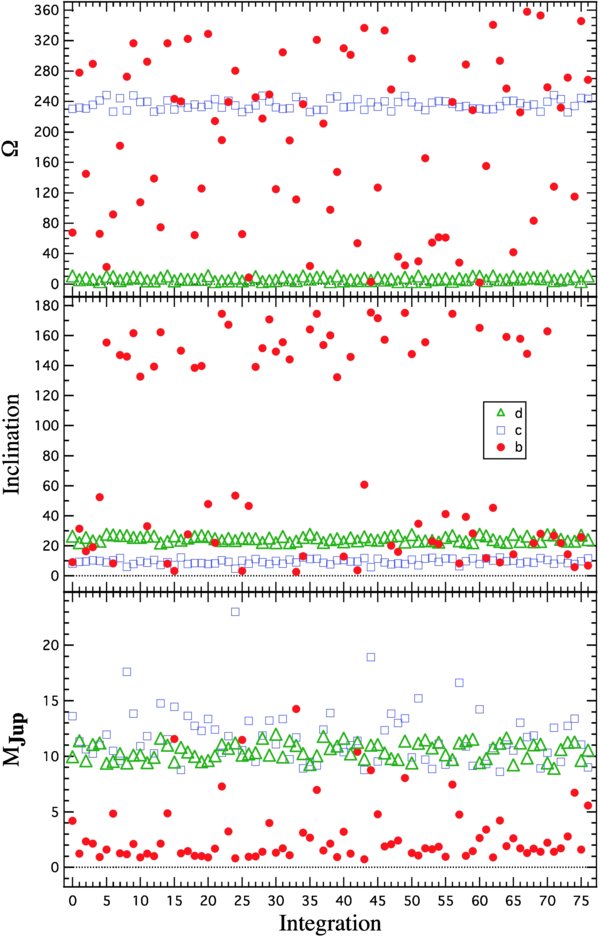
Figure 16. Plots detailing the 76 stable integrations of 100,000 years of the υ And system showing MJUP, inclination, and Ω for all three planets. Planets c and d used astrometric inputs for inclination and Ω sampled from a Gaussian distribution of error-adjusted values, while planet b used a uniform distribution of possible starting values. Note that Ωb is indeterminate and Mb is likely 1–2 MJUP.
Download figure:
Standard image High-resolution imageHNBody11 was then used to model the two- and three-planet system in order to examine orbital stability. Such a check is important because the values of eccentricity for both planets c and d have changed as more observations are made and also the mutual inclination has been determined. We now find larger values of eb and ec, as well as the large relative inclination. Moreover, a possible fourth, long-period planet may be present in the data, which may affect our best fit. With HNBody, we find the lowest χ2 fits from both Keplerian and n-body modeling are dynamically unstable (at least one planet is ejected) within 1 Myr. Therefore, we need to explore the parameter space around the determined elements.
As a first-order search for a stable configuration, we have integrated 300 systems that are consistent with the RV and astrometric data changing ed in the range 0.27–0.32, and varying the nodal configuration of b. We find that the dynamics are extremely complicated and depend sensitively on a secular resonance, general relativity and the oblateness of the central star (see, e.g., Adams & Laughlin 2006; Migaszewski & Gozdziewski 2009). The majority of the configurations we considered were unstable.
The evolution of e and I are shown for one example case in Figure 17 and Table 16 over 105 years. The left column shows the two-planet fit (i.e., planet b is not included). This solution is stable and evolves regularly for 100 Myr. The right column shows the three-planet fit. The evolutions of c and d appear to evolve regularly, however, planet b's eccentricity evolves aperiodically. This evolution suggests this configuration may be unstable on long timescales, but a million year integration was stable, and eb remained below 0.05 for the duration of the simulation. In this model, we included general relativity and a stellar oblateness of J2 = 10−3 and assumed a stellar radius of 1.26 R☉ (Migaszewski & Gozdziewski 2009).

Figure 17. Secular evolution of the fits presented in Table 16. The left panels show a system composed of just c (triangles, red) and d (crosses, blue). The right panel shows a plausible three-planet fit, with the nodal information of b (squares, green) chosen randomly.
Download figure:
Standard image High-resolution image
Table 16. Dynamical Stability: Example Two- and Three-planet Fits
| Planet | m (MJup) | a (AU) | e | I (°) | g(°) | ω (°) | M (°) |
|---|---|---|---|---|---|---|---|
| Two-planet Fit | |||||||
| c | 14.57 | 0.861 | 0.239 | 16.7 | 295.5 | 290.0 | 154.8 |
| d | 10.19 | 2.703 | 0.274 | 13.5 | 115.0 | 240.8 | 82.5 |
| Three-planet Fit | |||||||
| b | 5.9 | 0.0595 | 0.01 | 6.9 | 45.5 | 41.4 | 132.9 |
| c | 14.57 | 0.861 | 0.239 | 7.75 | 236.9 | 248.2 | 154.8 |
| d | 10.19 | 2.703 | 0.274 | 14.9 | 3.8 | 252.9 | 82.5 |
Download table as: ASCIITypeset image
Although the two-planet fit is acceptable, the three-planet fit needs refinement. An exhaustive search of parameter space (including J2) is beyond the scope of this investigation, but will be presented in a forthcoming paper (R. Barnes et al. 2010, in preparation). Given the complexity of the dynamics, it is conceivable that a stable, three-planet fit is consistent with the combined RV and astrometric observations.
These results should not be taken to mean that we have found the system as it is self-disrupting, rather the system probably lies very close to the stability boundary and the random errors in the observations led to the best-fit settling on an unstable configuration. Alternatively, the influence of the fourth (and possibly more) planet and the perturbations of υ And B may be adversely affecting our fits (potentially increasing the eccentricities of the confirmed planets) and hence our dynamical models as well. These issues will be addressed in R. Barnes et al. (2010, in preparation).
6. DISCUSSION
6.1. Previous and Current Astrometric Studies of the υ And System Compared
HIPPARCOS (HIP) made 27 visits to υ And, all one-dimensional measurements that were projected star positions on its instantaneous reference circle. The HIP intermediate astrometric data (IAD) has been used in several studies to estimate the mass or upper mass limits of some of the υ And planets. These studies typically held the published RV orbits (of the time) and the HIP parallax as constants, and then used various techniques to derive astrometric orbital elements (e.g., inclination) that were not measurable in the HIP data (as they are in the HST data).
In the first HIP study of υ And d by (Mazeh et al. 1999, MZ99), a valley in χ2 was found for α at 1.4 mas across all possible inclinations. The α was found to be 1.4 mas ± 0.6 mas, and the deduced (astrometrically undetectable) inclination was 156°+8−25 for a one-sigma mass estimate of 10.1−4.6+4.7 MJUP.12 The inclination (because it could not be measured) was derived from an equation using K and the inclination predicted from the minimum χ2 of that equation. In 2001, a similar process was used by Han et al. (2001) for mass estimations limits, except that in this process the asin i derived from the RV was fixed from the beginning. They also ignored the error in the spectroscopic elements. They found an α of 1.38 mas ± 0.64 mas and an inclination of 1555 (no error) and a mass of 108 MJUP. It is unclear how such a large mass was derived for υ And d, unless it was a typo.
Later in 2001, (Pourbaix 2001, P01) re-examined these earlier results, and found that some small inclinations found were merely artifacts of the fitting procedure that was used. P01 found that fitting (i, Ω) to the HIP IAD when the Aasin i is much smaller than the astrometric precision always yields low values of sin i, regardless of the true inclination. He found for υ And d using Aasin i as a constraint an inclination of 287 ± 168 and for υ And c an inclination of 172° ± 38; his F-test rejected both of these values at 20% and 23%, respectively. His test was the probability of obtaining an F-value greater or equal to the value found in the absence of a signal in the IAD (a false positive).
The parallax and proper motion results for υ And (see Table 10) illustrate that for this object, HST has achieved significantly more precise results (a parallax error of 0.1 mas for HST versus 0.72 mas for HIP) than HIP. We have enough data in this study to have confidence in signals that are as small as 0.25 mas. For our analysis, we do use a constraint in the relationship between the astrometry and the RV (see Equation (8)). Our modeling is significantly different than the modeling of the HIP IAD, however. We hold no orbital or astrometric parameters as constants. Our solutions do not converge unless there is a measurable signal, as discussed in Section 4.2. It is meaningful to note that the value of α for υ And d found by MZ99 (1.4 mas ± 0.6 mas) is within the errors equal to our HST determined value (1.385 mas ± 0.072 mas) and the mass estimate from MZ99, 10.1+4.7−4.6 MJUP, is very close to ours, 10.25+0.7−3.3 MJUP. Though MZ99, found an inclination of 156°+8−25 for υ And d, P01 found 287 ± 168, a value he did not have confidence in, but which compares favorably with the HST value of 23758 ± 1316. We note that for the MZ99 inclination of 156°, 180°−156°= 24°, the HST value. Our determination of astrometric elements and mass for υ And d confirm the much earlier determination by MZ99 and P01.
In retrospect, it is worth noting that almost all of the stability analyses carried out on the υ And system did not consider or mention the mass of υ And d determined in 1999, but instead used the significantly smaller minimum masses derived from the RV.
6.2. Possible Mass and Inclination of υ And b
υ And b is a hot Jupiter (a minimum mass of ∼ 0.7 MJUP) in a near-circular orbit. Nagasawa et al. (2008) found that an inner planet such as υ And b can re-enter a Kozai cycle, and that this repeated mechanism can improve the chances for tidal circularization to occur. υ And b is thought to have a hot day side and a cool night side, a "pM" class planet, in contrast to the "pL" class planets (represented by HD189733 b; pM–pL reference Fortney et al. 2008). Its infrared brightness was measured by Spitzer Space Telescope at five epochs and analyzed by Harrington et al. 2006, in which they proposed a consistent picture of the atmospheric energetics as long as the inclination is >30°.
While it was not possible to measure the inclination or astrometric signal α from υ And b (see Figure 7; which is most certainly in the low-microarcsecond regime) with HST, our dynamical stability analysis suggests possible masses (see Figure 16). υ And b may have a mass of MP= 1.4 MJUP (the minimum mass from RV is ∼0.7 MJUP) with an inclination around 25°. Without knowledge of Ω, we cannot estimate the mutual inclination.
6.3. The Astrophysical Implications
The υ And system presented itself, through its RV orbital elements, as an intriguing and theory-provoking system in 1999. It was a system with three Jupiter-mass-sized objects, the outer two having higher eccentricities, the inner surprisingly circular, which appeared to be on the edge of instability from dynamical analyses (Barnes & Quinn 2001). Studies focused on the existence of planet b in its circular orbit (Nagasawa & Lin 2005; Adams & Laughlin 2006), and the mechanism that excited the eccentricities of planets c and d (Lissauer & Rivera 2001; Chiang et al. 2001, 2002).
While early studies (Chiang et al. 2002) declared the gravitational interactions between υ And c and d are to "excellent approximation" secular, more recent studies (Migaszewski & Gozdziewski 2009) have found that "there is no simple and general recipe to predict the behavior of the secular system," that even in systems without extreme parameters the phase space of the modeling changes, and more branches of stable solutions are revealed. The finding by Adams & Laughlin (2006) that the addition of general relativity to the dynamic modeling damps the evolutionary growth of eccentricity in planet b is fundamental. This showed that incomplete stability modeling could erroneously makes an observed system seem improbable, if not impossible.
While most studies suggested that an outside player—another planet, a star, or the circumstellar disk—was directly responsible for the evolution of the eccentricities of planets c and d, there was a difference in interpretation based upon assumptions researchers made about the system. Assuming an Occum's razor position that the system is coplanar, Chiang et al. (2002) considered that interactions of the outer planet d with the circumstellar disk of gas provided for the amplification of eccentricities. Most others (Rivera & Lissauer 2000; Ford et al. 2005; Barnes & Greenberg 2006a) regard a planet as the likely accelerant. While a planet-scattering model (Ford et al. 2005) was found to be the simple explanation of the eccentricity amplification, a more explicit "rogue planet model" (Barnes & Greenberg 2007) was found to be necessary for the "near-separatix" state of the system. But both of these scenarios were based upon assumptions about the masses of planets c and d, based upon the RV minimum mass estimates (Msin ic = 1.8898+0.12−0.12MJUP and Msin id = 4.1754+0.26−0.27MJUP), and therefore assumed that the mass of planet d was larger than planet c. In MMR crossing between planets on divergent orbits (Chiang et al. 2002) and in close encounters between planets (Ford et al. 2001), the greater eccentricity is bestowed upon the least massive planet, and because of this assumption of a more massive planet d, an external source was needed. But, our astrometric measurements have shown that it is planet c (Mc = 13.98+2.3−5.3 MJUP) that is likely the more massive planet (Md = 10.25+0.73−3.27 MJUP) 13 thus altering the foundation for the theories used to explain the system that was "seen" with RV orbit alone (higher eccentricity of higher Msin i companion) but not expected (higher eccentricity on lower mass companion). The astrometric orbital elements turned the seen from unexpected to expected.
We find inclinations of υ And c to be 79 ± 1° and υ And d to be 238 ± 1°. For the first time, measurements of astrometric orbital elements of an extrasolar planetary system have been made to find the mutual inclination between planets. This is not a value derived from dynamical analysis as that of Bean & Seifahrt (2009); the signal of GL876 b is in the microsecond of arc range, far too small to have been detected or measured by HST astrometry, but it could be detected in the future by SIM.
The mutual inclination of υ And c and d is 299 ± 1°. Gas disk processes probably cannot pump mutual inclinations much above the opening angle of ≲5° (see, e.g., Ida & Lin 2004), but previous investigations of planet–planet scattering (Marzari & Weidenschilling 2002; Chatterjee et al. 2008) have easily produced such mutual inclinations. However, we cannot rule out a Kozai-type interaction (see, e.g., Kozai 1962; Takeda et al. 2008; Libert & Tsiganis 2009) with υ And B. Its orbit is poorly constrained, but if it is near the apocenter of an extremely eccentric and significantly inclined orbit, then it may be able to induce the observed mutual inclination. As the Kozai origin requires specific, low probability events, but the scattering naturally and easily explains the tight packing (Raymond et al. 2009) and large mutual inclination, we suggest that planet–planet scattering more likely produced the observed configuration.
We now have two planetary systems in which the actual mass and spatial relationship between two planets have been measured, our own solar system and the υ And system. These systems contain very different planetary objects at different distances and display contrasting architecture. The υ And planetary system seems to lie even closer to the stability boundary than previously thought (see, e.g., Laughlin & Adams 1999; Barnes & Quinn 2001; Barnes & Raymond 2004; Goździewski et al. 2001). Such a proximity to instability may seem startling, but could fit well with the planet–planet scattering models (Raymond et al. 2009).
Questions remain. Does the model of planet–planet scattering (Ford et al. 2005) provide a mechanism for excitation of eccentricity and mutual inclination that we measured in the υ And system, or does a modified theory of late-stage scattering of protoplanets (Barnes & Greenberg 2007) explain both the υ And system and our own solar system better? Could the divergence of their current state have been seeded during late formation or is it a product of the evolution of these systems? During the formation of the giant planets in υ And, could the interactions which formed the cores of these planets drive them into a higher mutual inclination state? Does the residual gas disk after planet formation also contribute to what we see? What mechanism keeps this system that appears to lie on the edge of stability stable?
6.4. The Importance of Astrometric Follow-up of Extrasolar Systems
The astrometric determination of the mass of a low-mass companion can decisively characterize it as a planet and reveal its hierarchical position in a planetary system. A good illustration of this fact can be seen from the results of our group for three objects that were previously listed as extrasolar planet candidates: Gliese 876 b, HD 136118 b, and HD 33636 b. Surprisingly, each object has been found to belong to a different class: a giant planet, a brown dwarf, and an M dwarf star, respectively, Benedict et al. (2002), Martioli et al. (2010), and Bean et al. (2007). These results demonstrate the importance of the application of complementary techniques in observing extrasolar planetary systems.
The measurements of the actual masses and the inclination of υ And c and d provide a new foundation for future theoretical and dynamical studies of our first uncovered extrasolar planetary system.
We thank Jacob Bean for the reductions from and implementation of our radial velocity pipeline, and Amber Armstrong and Aaron Juarez for their assistance in the processing of this data. We thank Matt Giguere, Debra Fischer, Howard Isaacson, and Geoff Marcy for the re-reduced Lick data. We thank Dominique Naef for the Elodie data. Support for this work was provided by NASA through grants GO-09971, GO-10103, and GO-11210 from the Space Telescope Science Institute, which is operated by the Association of Universities for Research in Astronomy (AURA), Inc., under NASA contract NAS5-26555. This publication makes use of data products from the Two Micron All Sky Survey, which is a joint project of the University of Massachusetts and the Infrared Processing and Analysis Center/California Institute of Technology, funded by NASA and the NSF. This research has made use of the SIMBAD database, operated at CDS, Strasbourg, France, and the NASA Astrophysics Data System Abstract Service.
This research is partially based on observations carried out with the Hobby-Eberly Telescope at McDonald Observatory.
Facilities: HET(HRS) - McDonald Observatory's Hobby-Eberly Telescope, HST - Hubble Space Telescope satellite
Footnotes
- *
Based on observations made with the NASA/ESA Hubble Space Telescope, obtained at the Space Telescope Science Institute, which is operated by the Association of Universities for Research in Astronomy, Inc., under NASA contract NAS5-26555. Based on observations obtained with the Hobby-Eberly Telescope, which is a joint project of the University of Texas at Austin, the Pennsylvania State University, Stanford University, Ludwig-Maximilians-Universitt Mnchen, and Georg-August-Universität Göttingen.
- 7
A detailed Instrument Handbook can be found on the Space Telescope Science Institute Web site: http://www.stsci.edu/hst/fgs/documents/instrumenthandbook/.
- 8
- 9
The Two Micron All Sky Survey is a joint project of the University of Massachusetts and the Infrared Processing and Analysis Center/California Institute of Technology.
- 10
- 11
Publicly available at http://janus.astro.umd.edu/HNBody/.
- 12
The mass of υ And used in the HIP mass calculation was not given in MZ99.
- 13
We note that it is possible within the errors that υ And c could have a lower mass than υ And d.