


ABSTRACT
We present the results of a three year monitoring program of a sample of very low mass (VLM) field binaries using both astrometric and spectroscopic data obtained in conjunction with the laser guide star adaptive optics system on the W. M. Keck II 10 m telescope. Among the 24 systems studied, 15 have undergone sufficient orbital motion, allowing us to derive their relative orbital parameters and hence their total system mass. These measurements more than double the number of mass measurements for VLM objects, and include the most precise mass measurement to date (<2%). Among the 11 systems with both astrometric and spectroscopic measurements, six have sufficient radial velocity variations to allow us to obtain individual component masses. This is the first derivation of the component masses for five of these systems. Altogether, the orbital solutions of these low mass systems show a correlation between eccentricity and orbital period, consistent with their higher mass counterparts. In our primary analysis, we find that there are systematic discrepancies between our dynamical mass measurements and the predictions of theoretical evolutionary models (TUCSON and LYON) with both models either underpredicting or overpredicting the most precisely determined dynamical masses. These discrepancies are a function of spectral type, with late-M through mid-L systems tending to have their masses underpredicted, while one T-type system has its mass overpredicted. These discrepancies imply that either the temperatures predicted by evolutionary and atmosphere models are inconsistent for an object of a given mass, or the mass–radius relationship or cooling timescales predicted by the evolutionary models are incorrect. If these spectral-type trends are correct and hold into the planetary mass regime, the implication is that the masses of directly imaged extrasolar planets are overpredicted by the evolutionary models.
Export citation and abstract BibTeX RIS
1. INTRODUCTION
Characterizing the fundamental properties of brown dwarfs is an important step in unlocking the physics of substellar objects. These very cool objects have internal and atmospheric properties that are quite similar to gas giant planets and that differ fundamentally from those of stars, including partially degenerate interiors, dominant molecular opacities, and atmospheric dust formation (Chabrier & Baraffe 2000). Brown dwarfs also represent a substantial fraction of the galactic stellar content, and are bright and numerous enough to be studied in great detail with current technology (Kirkpatrick 2005). Thus, these substellar objects present an ideal laboratory in which to study the physical processes at work in very low mass (VLM) objects that both approach and overlap the planetary mass regime.
Mass is the most fundamental parameter in determining the properties and evolution of a brown dwarf; unfortunately, it is also one of the most difficult to measure. Masses of brown dwarfs are typically inferred from the comparison of measured luminosities and temperatures with predictions from theoretical models. The most commonly used models are those of Burrows et al. (1997) and Chabrier et al. (2000). However, as shown in Figure 1, masses obtained in this way from different models can be discrepant, especially amongst the lowest mass objects. These discrepancies stem from physical assumptions about the interior and atmospheric properties of these highly complex objects. Examples of uncertainties in the models are atmospheric processes that define the transition regions between spectral types. Specifically, this includes the formation of atmospheric clouds (M to L), the disappearance of clouds (L to T), and the formation of ammonia, which makes the objects, in theory, similar atmospherically to Jupiter (T to Y). Additional sources of uncertainties in the models include, but are not limited to, the equation of state (Chabrier & Baraffe 2000), the initial conditions and accretion history (Baraffe et al. 2009), the treatment of convection and the possible subsequent generation of magnetic fields, which in turn could affect the inferred effective temperatures (Chabrier & Kuker 2006; Browning 2008). An essential step toward properly calibrating these models and constraining their physics is to obtain high precision (≲10%) dynamical mass measurements of brown dwarf binaries.

Figure 1. Percent discrepancy in mass predictions between the Burrows et al. (1997) evolutionary and the Chabrier et al. (2000) evolutionary models, over the range on the H–R diagram with complimentary coverage. The colors represent the level of the discrepancy in units of percent of the mass predicted by the Burrows et al. (1997) models, as shown by the scale bar. For the majority of the H–R diagram, the discrepancy between the model predictions is ≳10%, with a number of regions having discrepancies greater than 100%. Overplotted are two isochrones and lines of constant mass from the Burrows et al. (1997) models for points of reference. In addition, the overplotted filled points show the rough location of the sources in our full sample. The largest discrepancies are at the youngest ages, but the discrepancies are still substantial for older objects.
Download figure:
Standard image High-resolution imageThe advent of laser guide star (LGS) adaptive optics (AO) on large ground-based telescopes has dramatically increased the number of VLM objects for which high-precision dynamical masses can be obtained. Prior to AO, only one binary brown dwarf had sufficiently precise mass measurements to test the models and this was the case of Two Micron All Sky Survey (2MASS) J053521840546085, an eclipsing binary in Orion, which provided constraints at a very young age (∼Myr; Stassun et al. 2006). Early AO, which used natural guide stars, allowed dynamical mass estimates for two brown dwarfs (Lane et al. 2001; Zapatero Osorio et al. 2004; Simon et al. 2006; Bouy et al. 2004). With LGS AO, much fainter sources can be targeted, allowing ∼80% of known brown dwarf binaries to be observed and a much more systematic look at how the observed properties of brown dwarfs compare with the predictions of models.
To capitalize on the introduction of LGS AO on 10 m class telescopes, we initiated, in 2006, an extensive astrometric and spectroscopic monitoring campaign of 23 VLM binaries (Mtot≲ 0.2 M☉) in the near-infrared with the Keck/LGS-AO system with the goal of obtaining precision dynamical masses. The astrometric aspect of this project is similar to the work reported on three individual targets by Liu et al. (2008) and Dupuy et al. (2009a, 2009b, 2009c). Our survey includes these targets as well as others to span a wide range of late stellar and substellar spectral types (M7.5 to T5.5) and is the first study to include radial velocity measurements for the LGS AO targets. Our relative astrometric and radial velocity measurements provide estimates of the total system mass for 15 systems. Our absolute radial velocity measurements, add estimates of the mass ratios and hence individual mass estimates for six of these systems. Altogether, this work more than doubles both the current number of system mass measurements and individual mass estimates for VLM objects and, when compared to the models, shows systematic discrepancies.
This paper is organized as follows. Section 2 describes the sample selection and Section 3 provides a description of the astrometric and spectroscopic observations. Section 4 outlines the data analysis procedures and Section 5 describes the derivation of orbital solutions. Section 6 contains the estimates of bolometric luminosities and effective temperatures for the components of the binaries. Section 7 compares the dynamical masses to the predictions from evolutionary models and the implications of our model comparison are discussed in Section 8. We summarize our findings in Section 9.
2. SAMPLE SELECTION
2.1. Initial Sample
The initial sample for this project was culled from Burgasser et al. (2007), which listed the 68 visual, VLM binaries known as of 2006.10 Three cuts were applied to this initial list. First, the binaries had to be observable with the Keck telescope LGS AO system, so we imposed a declination >−35° requirement, which reduced the possible number of targets to 61. Second, the operation of the LGS AO system requires a tip-tilt reference source of apparent R magnitude <18 within an arcminute of the source, and therefore VLM binaries without a suitable tip-tilt reference were also cut. This lowered the total number of observable targets to 49, 80% of the northern hemisphere sample.
Third, we required that useful dynamical mass estimates would likely be obtained within three years. To assess the required precision for our dynamical mass estimates, we calculated the predicted masses for the two most commonly used sets of evolutionary models, those of Burrows et al. (1997) and Chabrier et al. (2000), across the entire range of temperatures and luminosities spanned by both models. We calculated the percent difference between the predictions of each model with respect to the prediction of Burrows et al. (1997). The results of this assessment are shown in Figure 1, which displays in color the offset between the models across the Hertzsprung–Russell (H–R) diagram (with the discrepancies averaged in 50 K temperature increments and 0.1 log(L/L☉ increments). As the figure demonstrates, we found that the difference in the mass predictions of the two models varied anywhere from a few percent to greater than 100%. We therefore chose a precision goal of 10% because at this level the majority of the model predictions could be distinguished and because this level of precision was reasonable to expect given our observing strategy.
To implement our third cut, a series of Monte Carlo simulations were performed. In these simulations, the total system mass for each target was assumed based on the estimated spectral types of the binary components from the original discovery papers, using the Chabrier et al. (2000) models, and held constant for all runs. Additionally, the semimajor axis of the orbit was chosen by sampling from the range of possible values between 1/2 and 2 times the original separation measurement. From these assumptions, a period was calculated, and To (time of periapse passage) was randomly selected from the range allowed by this period. All other orbital parameters for an astrometric orbit, which include e (eccentricity), i (inclination), Ω (longitude of the ascending node), and ω (argument of periapsis), were randomly selected from among the complete range of possible values of each parameter.
Using these simulated orbits, it was possible to generate simulated sets of "astrometric data points" corresponding to the likely times of measurement. We planned on two observing campaigns per year, one in June and the other in December. These dates were chosen to coincide with the 2 times per year that NIRSPEC is offered behind the LGS AO system at Keck (see Section 3). The sky coordinates of each binary then determined whether we simulated one or two astrometric and radial velocity data points per year. These simulated measurements were chosen to correspond to appropriate observing dates. All synthetic data points were combined with already existing measurements, the number of which varied from source to source. While the majority of sources initially had only one previous astrometric measurement, a few had up to six. Synthetic astrometric data points were also assigned uncertainties based on the average uncertainty normally obtained for short-exposure measurements of binary stars using the Keck AO system with NIRC2 (σ∼ 1 mas). Although the average uncertainty in relative radial velocity measurements with NIRSPEC+AO (NIRSPAO) was not known at the time, other observations with NIRSPEC suggested using a conservative uncertainty of about 1 km s−1. All data points were then used to run the orbital solution fitter, which uses the Thiele–Innes method (e.g., Hilditch 2001), minimizing the χ2 between the model and the measurements (see Ghez et al. 2008). A chi-squared cut of 10 was imposed to account for the fact that in some simulated orbital solutions we could not generate astrometric measurements corresponding to real data points in those systems with multiple measurements. In this way, we were able to utilize more information than simply separation and estimated mass to calculate likelihood of accurate mass measurement in a system. A total of 1000 simulated orbital solutions were created for each system.
From each of these simulations, the predicted uncertainty in dynamical mass could be determined. All those systems for which 66% of the simulations yielded precisions of 10% or better in mass were put in the final sample. This generated a sample of 21 targets that we began monitoring in the spring of 2006. These sources are listed in Table 1. Figure 2 shows the results of our simulations, plotting the percent of solutions with precise mass estimates versus the initial binary separation. The spectral type of the primary component is denoted by symbol shape, and sources included in our initial sample are colored red. The variation in percent of solutions with separation stems from the variation in the estimated masses of the components and the number of previous measurements at the start of our monitoring program.

Figure 2. Percent of solutions in our Monte Carlo simulations that yielded a mass with ≲10% precision vs. the initial separation of the binary. Sources included in our sample are denoted in red, with the red dotted line showing our cutoff of 66%. Additional sample members are denoted in blue and were chosen because they had either L or T spectral types and because they had a probability of >50% of yielding a precise mass in our initial simulations (with an increased probability for high precision masses by 2012). Sources which were not included in the original Monte Carlo simulation because of their later discovery epoch, but that have a high likelihood of yielding a precise mass by 2012, are shown in green. The symbol type denotes the spectral type of the primary component.
Download figure:
Standard image High-resolution imageTable 1. VLM Binary Sample
| Source Name | R.A. | Decl. | Estimated | Discovery | 2MASS |
|---|---|---|---|---|---|
| (J2000) | (J2000) | Sp Typesa | Reference | K-band Magnitude | |
| LP 349-25AB | 00 27 55.93 | +22 19 32.8 | M8+M9 | 11 | 9.569 ± 0.017 |
| LP 415-20AB | 04 21 49.0 | +19 29 10 | M7+M9.5 | 7 | 11.668 ± 0.020 |
| 2MASS J05185995−2828372ABb | 05 18 59.95 | −28 28 37.2 | L6+T4 | 1 | 14.162 ± 0.072 |
| 2MASS J06523073+4710348ABb | 06 52 30.7 | +47 10 34 | L3.5+L6.5 | 2 | 11.694 ± 0.020 |
| 2MASS J07003664+3157266 | 07 00 36.64 | +31 57 26.60 | L3.5+L6 | 2 | 11.317 ± 0.023 |
| 2MASS J07464256+2000321AB | 07 46 42.5 | +20 00 32 | L0+L1.5 | 3 | 10.468 ± 0.022 |
| 2MASS J08503593+1057156 | 08 50 35.9 | +10 57 16 | L6+L8 | 3 | 14.473 ± 0.066 |
| 2MASS J09201223+3517429AB | 09 20 12.2 | +35 17 42 | L6.5+T2 | 3 | 13.979 ± 0.061 |
| 2MASS J10170754+1308398ABc | 10 17 07.5 | +13 08 39.1 | L2+L2 | 4 | 12.710 ± 0.023 |
| 2MASS J10210969−0304197 | 10 21 09.69 | −03 04 20.10 | T1+T5 | 13 | 15.126 ± 0.173 |
| 2MASS J10471265+4026437AB | 10 47 12.65 | +40 26 43.7 | M8+L0 | 5 | 10.399 ± 0.018 |
| GJ 569b AB | 14 54 29.0 | +16 06 05 | M8.5+M9 | 12 | ∼9.8 |
| LHS 2397a AB | 11 21 49.25 | −13 13 08.4 | M8+L7.5 | 10 | 10.735 ± 0.023 |
| 2MASS J14263161+1557012AB | 14 26 31.62 | +15 57 01.3 | M8.5+L1 | 5 | 11.731 ± 0.018 |
| HD 130948 BC | 14 50 15.81 | +23 54 42.6 | L4+L4 | 9 | ∼11.0 |
| 2MASS J15344984−2952274AB | 15 34 49.8 | −29 52 27 | T5.5+T5.5 | 6 | 14.843 ± 0.114 |
| 2MASS J1600054+170832ABb | 16 00 05.4 | +17 08 32 | L1+L3 | 4 | 14.678 ± 0.114 |
| 2MASS J17281150+3948593AB | 17 28 11.50 | +39 48 59.3 | L7+L8 | 4 | 13.909 ± 0.048 |
| 2MASS J17501291+4424043AB | 17 50 12.91 | +44 24 04.3 | M7.5+l0 | 7 | 11.768 ± 0.017 |
| 2MASS J18470342+5522433AB | 18 47 03.42 | +55 22 43.3 | M7+M7.5 | 8 | 10.901 ± 0.020 |
| 2MASS J21011544+1756586 | 21 01 15.4 | +17 56 58 | L7+L8 | 4 | 14.892 ± 0.116 |
| 2MASS J21402931+1625183AB | 21 40 29.32 | +16 25 18.3 | M8.5+L2 | 5 | 11.826 ± 0.031 |
| 2MASS J21522609+0937575 | 21 52 26 | +09 37 57 | L6+L6 | 2 | 13.343 ± 0.034 |
| 2MASS J22062280−2047058AB | 22 06 22.80 | −20 47 05.9 | M8+M8 | 5 | 11.315 ± 0.027 |
Notes. aFrom discovery reference. bIn all observations of these sources, the binary was never resolved. We report upper limits to the separations of these binaries, but no orbital solutions can be derived. cSource cut from sample due to additional astrometry showing that it was not likely to yield a mass to a precision of better than 10% in the required timeframe. References. (1) Cruz et al. 2004; (2) Reid et al. 2006; (3) Reid et al. 2001; (4) Bouy et al. 2003; (5) Close et al. 2003; (6) Burgasser et al. 2003; (7) Siegler et al. 2003; (8) Siegler et al. 2005; (9) Potter et al. 2002; (10) Freed et al. 2003; (11) Forveille et al. 2005; (12) Martín et al. 2000; (13) Burgasser et al. 2006.
Download table as: ASCIITypeset image
2.2. Sample Refinement
Upon commencement of the monitoring campaign, it became clear that sample refinement and adjustment of observing priorities was required. Three sources had tip/tilt stars that did not allow for successful observation (2MASS 0423−04, GJ 417B, and 2MASS 1217−03). It is possible that some of these tip/tilt stars were actually resolved galaxies. In addition, 2MASS 1217−03 was later re-observed with Hubble Space Telescope (HST) and found to be unresolved, making it unlikely to be a binary (Burgasser et al. 2006). Therefore, we monitored 19 of the 22 initially identified brown dwarfs.
Additionally, a few targets were added to the monitoring program as it progressed. First, it was recognized that some sources did not make the cut because of the three year timescale constraint, but with a slightly longer period of monitoring could have their masses derived to a high level of accuracy. In particular, the timescale cut introduced an obvious bias to sources with higher predicted masses, or earlier spectral types. Therefore, we added three objects included in Burgasser et al. (2007) to the NIRC2 monitoring program to provide initial epochs of data for future mass determination. These three objects are shown in Figure 2 in blue. All three were of spectral type L or T (we did not add additional M dwarfs to our sample because of the large number of M dwarfs included in our initial sample). All three had a >50% probability of a precise dynamical mass estimate in our initial Monte Carlos. These added sources are noted in Table 1. Two additional sources were added to the sample that were discovered by Reid et al. (2006) after the initial publication of Burgasser et al. (2007). For these sources, we have calculated the likelihood that they will yield precise mass estimates by 2012. These sources are denoted in Figure 2 in green to keep them distinct from the sources from our initial simulations, as we calculated their likelihood of yielding a good mass estimate by 2012 instead of 2009. We found that both sources had a >50% chance of yielding a precise mass estimate by 2012, and therefore added these two sources to our astrometric program. They are also listed in Table 1.
3. OBSERVATIONS
3.1. Astrometric Data
Targets in our sample were observed astrometrically beginning in 2006 May. Observations were conducted twice a year between 2006 May and 2009 June UT using the Keck II 10 m telescope with the facility LGS AO system (Wizinowich et al. 2006; van Dam et al. 2006) and the near-infrared camera, NIRC2 (PI: K. Matthews). The AO system, which is also used for obtaining radial velocities (see the next section), uses the sodium laser spot (V∼10.5) as the primary correction source for all but two systems. Tip/tilt references are listed in Table 2. NIRC2 has a plate scale of 9.963 ± 0.005 mas pixel−1 and columns that are at a position angle (P.A.) of 0.13 ± 0 02 relative to north (Ghez et al. 2008). The observing sequence for each object depended upon the brightness of the target, whether observations in multiple filters had been previously made, and whether the target was actually resolved into two components at that epoch. If the binary was not resolved, we could only obtain an upper limit on the separation, which does not require a full observing sequence to estimate. We generally tried to take at least nine individual exposures on each target, though sometimes due to time constraints fewer exposures were taken. Table 2 gives the log of all imaging and photometric observations, listing when each target was observed, the filters through which it was observed and the exposure time and number of images taken in each filter, and the tip/tilt reference source used for each target. In many cases, the brown dwarf targets were bright enough to serve as their own tip/tilt reference, even though they are not bright enough for natural guide star observations.
Table 2. Log of NIRC2 LGS AO Observations
| Target | Date of | Tip/Tilt | Filter | Exposure Time | No. of |
|---|---|---|---|---|---|
| Name | Observation (UT) | Reference | (s × coadds) | Frames | |
| 2MASS 0518−28AB | 2006 Nov 27 | USNO-B1.0 0615-0055823 | Kp | 30 × 4 | 18 |
| 2007 Dec 2 | Kp | 30 × 4 | 9 | ||
| 2008 Dec 18 | Kp | 20 × 4 | 5 | ||
| 2MASS 0652+47AB | 2006 Nov 27 | USNO-B1.0 1371-0206444 | Kp | 8 × 12 | 6 |
| 2007 Dec 2 | Kp | 5 × 12 | 9 | ||
| 2MASS 0746+20AB | 2006 Nov 27 | Source | Kp | 2 × 30 | 9 |
| 2007 Dec 1 | Kp | 2 × 30 | 8 | ||
| 2007 Dec 1 | J | 4 × 15 | 9 | ||
| 2008 Dec 18 | Kp | 2 × 30 | 8 | ||
| 2008 Dec 18 | H | 2 × 30 | 6 | ||
| 2MASS 0850+10AB | 2007 Dec 2 | USNO-B1.0 1009-0165240 | Kp | 30 × 4 | 9 |
| 2008 Dec 18 | Kp | 10 × 1 | 5 | ||
| 2MASS 0920+35AB | 2006 Nov 27 | USNO-B1.0 1252-0171182 | Kp | 30 × 4 | 7 |
| 2007 Dec 2 | Kp | 30 × 4 | 4 | ||
| 2007 Dec 2 | J | 30 × 4 | 2 | ||
| 2008 May 30 | Kp | 30 × 4 | 6 | ||
| 2008 Oct 21 | H | 30 × 4 | 6 | ||
| 2008 Dec 18 | H | 10 × 10 | 7 | ||
| 2009 Jun 10 | H | 10 × 5 | 6 | ||
| 2MASS 1017+13AB | 2006 Nov 27 | USNO-B1.0 1031-0208442 | Kp | 13 × 12 | 3 |
| 2MASS 1047+40AB | 2006 Jun 21 | Source | Kp | 1 × 60 | 9 |
| 2006 Nov 27 | Kp | 2 × 30 | 12 | ||
| 2007 Dec 2 | Kp | 2 × 30 | 6 | ||
| 2008 Dec 18 | Kp | 1 × 30 | 9 | ||
| 2MASS 1426+15AB | 2006 Jun 20 | USNO B1.0-1059-0232527 | Kp | 10 × 12 | 3 |
| 2008 May 30 | Kp | 10 × 12 | 8 | ||
| 2008 May 30 | J | 15 × 5 | 5 | ||
| 2009 May 2 | Kp | 5 × 12 | 9 | ||
| 2009 May 2 | H | 5 × 12 | 6 | ||
| 2MASS 1534−29AB | 2006 Jun 20 | USNO-B1.0 0601-0344997 | J | 30 × 4 | 9 |
| 2008 May 30 | Kp | 40 × 2 | 7 | ||
| 2008 May 30 | H | 40 × 2 | 6 | ||
| 2008 May 30 | J | 40 × 1 | 3 | ||
| 2009 May 4 | H | 30 × 4 | 6 | ||
| 2MASS 1600+17AB | 2007 May 20 | USNO-B1.0 1071-0293881 | Kp | 30 × 4 | 9 |
| 2008 May 30 | Kp | 10 × 1 | 2 | ||
| 2MASS 1728+39AB | 2007 May 20 | USNO-A2.0 1275-09377115 | Kp | 30 × 4 | 5 |
| 2008 May 30 | Kp | 30 × 2 | 4 | ||
| 2008 May 30 | J | 60 × 2 | 5 | ||
| 2009 May 3 | Kp | 30 × 2 | 7 | ||
| 2009 Jun 11 | H | 30 × 4 | 9 | ||
| 2MASS 1750+44AB | 2006 Jun 20 | Source | Kp | 20 × 4 | 8 |
| 2007 May 17 | Kp | 10 × 12 | 7 | ||
| 2008 May 13 | Kp | 10 × 12 | 6 | ||
| 2008 May 30 | H | 5 × 12 | 6 | ||
| 2008 May 30 | J | 10 × 1 | 4 | ||
| 2009 May 1 | Kp | 5 × 12 | 9 | ||
| 2MASS 1847+55AB | 2006 May 21 | Source | Kp | 5 × 6 | 6 |
| 2007 May 14 | Kp | 1.452 × 1 | 9 | ||
| 2008 May 20 | Kp | 5 × 12 | 9 | ||
| 2008 May 20 | H | 5 × 5 | 6 | ||
| 2008 May 20 | J | 10 × 1 | 19 | ||
| 2009 May 4 | Kp | 5 × 12 | 9 | ||
| 2MASS 2140+16AB | 2006 May 21 | USNO-B1.0 1064-0594380 | Kp | 5 × 1 | 12 |
| 2006 Nov 27 | Kp | 10 × 12 | 9 | ||
| 2007 May 14 | Kp | 7 × 5 | 9 | ||
| 2007 Dec 2 | Kp | 10 × 12 | 9 | ||
| 2008 May 15 | Kp | 10 × 12 | 9 | ||
| 2008 May 30 | H | 5 × 12 | 4 | ||
| 2008 May 30 | J | 10 × 1 | 4 | ||
| 2008 Dec 19 | Kp | 5 × 12 | 9 | ||
| 2009 Jun 11 | Kp | 5 × 12 | 8 | ||
| 2MASS 2206−20AB | 2006 May 21 | Source | Kp | 5 × 6 | 9 |
| 2006 Nov 27 | Kp | 10 × 12 | 9 | ||
| 2007 May 17 | Kp | 10 × 3 | 8 | ||
| 2007 Dec 2 | Kp | 10 × 12 | 2 | ||
| 2008 May 30 | Kp | 5 × 12 | 9 | ||
| 2008 May 30 | H | 5 × 6 | 3 | ||
| 2008 May 30 | J | 10 × 1 | 6 | ||
| 2009 Jun 11 | Kp | 2.5 × 12 | 9 | ||
| GJ 569BC | 2009 Jun 11 | GJ569A | Kp | 0.5 × 30 | 10 |
| HD 130948BC | 2007 May 11 | HD 130948A | Kp | 2 × 30 | 12 |
| 2007 May 11 | H | 2 × 60 | 12 | ||
| 2007 May 11 | J | 4 × 15 | 12 | ||
| 2008 Apr 28 | Kp | 0.1452 × 1 | 12 | ||
| 2009 May 9 | H | 1 × 15 | 7 | ||
| LHS 2397aAB | 2006 Nov 27 | Source | Kp | 15 × 10 | 3 |
| 2007 Dec 2 | Kp | 8 × 15 | 3 | ||
| 2007 Dec 2 | J | 10 × 15 | 6 | ||
| 2008 May 30 | Kp | 3 × 30 | 8 | ||
| 2008 Dec 18 | Kp | 2 × 30 | 8 | ||
| 2008 Dec 18 | H | 1.5 × 30 | 6 | ||
| 2008 Dec 18 | J | 2 × 30 | 6 | ||
| 2009 Jun 10 | Kp | 2 × 30 | 9 | ||
| LP 349-25AB | 2006 Nov 27 | Source | Kp | 1 × 30 | 5 |
| 2006 Nov 27 | H | 1 × 30 | 5 | ||
| 2006 Nov 27 | J | 1.5 × 30 | 3 | ||
| 2007 Dec 2 | Kp | 5 × 6 | 9 | ||
| 2008 May 30 | Kp | 1.452 × 20 | 7 | ||
| 2008 Dec 19 | Kp | 2 × 20 | 6 | ||
| 2008 Dec 19 | J | 1.5 × 20 | 5 | ||
| 2009 Jun 11 | Kp | 0.5 × 20 | 12 | ||
| LP 415-20AB | 2006 Nov 27 | Source | Kp | 8 × 12 | 6 |
| 2007 Dec 2 | Kp | 6 × 12 | 9 | ||
| 2008 Dec 18 | Kp | 6 × 12 | 9 | ||
| 2008 Dec 18 | H | 5 × 12 | 9 |
With only a few exceptions, all data used for astrometry were taken through the K-prime (λo = 2.124 μm, Δλ = 0.351 μm) bandpass filter. Data in both the J band (λo = 1.248 μm, Δλ = 0.163 μm) and H band (λo = 1.633 μm, Δλ = 0.296 μm) were also taken at some point for most targets to provide a complete set of spatially resolved, near-infrared photometry. The images were generally taken in a three position, 2 5 × 25 dither box, with three exposures per position (avoiding the lower left quadrant of NIRC2, which has significantly higher noise than the other three), which allowed sky frames to be generated from the images themselves. In addition, the wide dither box insures the incorporation of known residual distortion (Ghez et al. 2008; S. Yelda et al. 2010, in preparation) in the camera into our final astrometric uncertainties.
3.2. Radial Velocity Data
Eleven objects (mK≲ 12) in our astrometric sample were also observed using the NIR spectrograph NIRSPEC on Keck II (McLean et al. 2000) in conjunction with the LGS AO system (NIRSPAO). We used the instrument in its high spectral resolution mode, selecting a slit 0041 in width and 226 in length in AO mode. We elected to observe in the K band, with a particular interest in the densely populated CO band head region (∼2.3 μm, order 33), necessitating an echelle angle of 63° and a cross-disperser angle of 3565. The resolution in this setup is R ∼ 23, 000, as determined by the width of unresolved OH sky lines, and the wavelengths covered are 2.044–2.075 μm (order 37), 2.100–2.133 μm (order 36), 2.160–2.193 μm (order 35), 2.224–2.256 μm (order 34), 2.291–2.325 μm (order 33), and 2.362–2.382 μm (order 32), with some portions of the K band beyond the edges of the detector. For this work, all analysis was done using only order 33, the order containing the CO bandhead, and all data presented come from this order.
The camera was rotated such that both components of each binary fell simultaneously on the high resolution slit, which is at an angle of 1059 with respect to north. Typical observations consisted of four spectra of both components, each with 1200 s integration times, taken in an ABBA dither pattern along the length of the slit. In a few cases, more than four spectra were taken or a slightly different integration time was used, depending on the brightness of the object. Table 3 gives the log of our spectroscopic observations, listing the targets observed, the date of observation, the number of spectra, and the integration time for each spectrum. We successfully obtained spatially resolved spectra for sources separated by ≳60 mas in all epochs. Each target observation was accompanied by the observation of a nearby A0V star to measure the telluric absorption in the target spectra.
Table 3. Log of NIRSPAO-LGS K-band Observations
| Target | Date of | A0V Star | Exposure Time | No. of |
|---|---|---|---|---|
| Name | Observation (UT) | Standard | (s × coadds) | Frames |
| 2MASS J07464256+2000321AB | 2006 Dec 16 | HIP 41798 | 1200 × 1 | 4 |
| 2007 Dec 4 | HIP 41798 | 1200 × 1 | 6 | |
| 2008 Dec 19 | HIP 41798 | 1200 × 1 | 6 | |
| 2MASS J14263161+1557012AB | 2007 Jun 8 | HIP 73087 | 1200 × 1 | 4 |
| 2008 Jun 1 | HIP 73087 | 1200 × 1 | 4 | |
| 2009 Jun 12 | HIP 73087 | 1200 × 1 | 4 | |
| 2MASS J17501291+4424043AB | 2008 May 31 | HIP 87045 | 1200 × 1 | 4 |
| 2009 Jun 12 | HIP 87045 | 1200 × 1 | 6 | |
| 2MASS J18470342+5522433AB | 2007 Jun 8 | HIP 93713 | 1200 × 1 | 4 |
| 2008 Jun 1 | HIP 93713 | 1200 × 1 | 5 | |
| 2009 Jun 13 | HIP 93713 | 1200 × 1 | 3 | |
| 2MASS J21402931+1625183AB | 2007 Jun 9 | HIP 108060 | 1200 × 1 | 4 |
| 2008 May 31 | HIP 108060 | 1800 × 1 | 3 | |
| 2009 Jun 13 | HIP 108060 | 1800 × 1 | 2 | |
| 2MASS J22062280−2047058AB | 2007 Jun 9 | HIP 116750 | 1200 × 1 | 3 |
| 2008 Jun 1 | HIP 109689 | 1200 × 1 | 4 | |
| 2009 Jun 12 | HIP 109689 | 1200 × 1 | 4 | |
| GJ 569b AB | 2007 Jun 9 | HIP 73087 | 900 × 1 | 2 |
| 2009 Jun 13 | HIP 73087 | 900 × 1 | 4 | |
| HD 130948BC | 2007 Jun 9 | HIP 73087 | 1200 × 1 | 4 |
| LHS 2397aAB | 2007 Dec 4 | HIP 58188 | 1800 × 1 | 2 |
| 2008 May 31 | HIP 61318 | 1800 × 1 | 3 | |
| 2008 Dec 19 | HIP 58188 | 1800 × 1 | 3 | |
| 2009 Jun 12 | HIP 61318 | 1800 × 1 | 2 | |
| LP 349-25AB | 2006 Dec 16 | HIP 5132 | 600 × 1 | 4 |
| 2007 Dec 4 | HIP 5132 | 900 × 1 | 1 | |
| 2008 Dec 19 | HIP 5132 | 1200 × 1 | 4 | |
| 2009 Jun 12 | HIP 5132 | 1200 × 1 | 4 | |
| LP 415-20AB | 2008 Dec 19 | HIP 24555 | 1200 × 1 | 4 |
Download table as: ASCIITypeset image
4. DATA ANALYSIS
4.1. Astrometric Data Analysis
The NIRC2 data were initially processed using standard data reduction techniques for near-infrared images. Frames at differing dither positions were subtracted from each other to remove sky background, followed by the removal of bad pixels, division by a flat field, and correction for optical distortion with a model provided in the pre-ship review document11 using standard IRAF and IDL routines. The binaries were then shifted to a common location in all frames and the images were median combined. Astrometry and flux ratios were obtained using the IDL package StarFinder (Diolaiti et al. 2000). An empirical point-spread function (PSF) is required by the StarFinder fitting algorithm. In the case of two sources, a suitable PSF star falls within the field of view of the NIRC2 observation of the source. However, in the majority of cases, no such PSF source is in the field of view. For these observations, we use either an image of a single star taken near in time to the images of the binary, or if no suitable single star was imaged, we use an idealized Keck PSF degraded to the calculated Strehl ratio of the observation for PSF fitting. For this last case, the PSF is generated by first convolving the idealized PSF with a Gaussian, such that the core is broadened to the appropriate FWHM. Next, a simulated "halo" is generated by adding a Gaussian with FWHM of 05 (average near-infrared seeing halo at Keck), normalized such that the resulting Strehl ratio matches the observations. Internal statistical measurement errors were calculated by fitting the components of the binaries in all individual images that contributed to the combined images and finding the rms of the values derived therein.
Additional systematic uncertainties need to be accounted for when determining the final astrometric and photometric measurements for each binary. First, absolute uncertainties in the plate scale and position of north given above are accounted for in all astrometry. A further, more complicated, source of uncertainty stems from using a PSF that is not imaged simultaneously with each binary, introducing systematic uncertainties in both astrometry and photometry. In particular, the variability of the AO performance over a given night generates time variable PSF structure that can contribute to slight offsets in astrometry and photometry. To estimate the additional uncertainty due to imperfect PSF matching, we performed simulations in which 1000 artificial binaries were generated using images of image single sources with separations and flux ratios spanning the range observed for our sources. These artificial binaries were then fit with StarFinder using either a separate single source from the same night or simulated source as the PSF. This exercise was performed for every night in which observations were taken for both PSF types. Examples of the results of these simulations are shown in Figure 3 (from the night of 2006 May 21). We find in all simulations that median offsets between input and fitted separations are an exponentially decreasing function of the separation, meaning that fits to tighter binaries were more discrepant from the correct values than those to wide binaries. We also find that due to variable structure in AO PSF halos (even after accounting for pupil rotation), the offset in fitted P.A. is a function of the P.A. of the binary. Finally, the median offset in fitted flux ratio with respect to the input flux ratio was essentially constant for all separations and P.A.s. Therefore, for every measurement of each target, we compute the necessary uncertainties from imperfect PSFs based on the relationships detailed above, taking the median values of the measured offsets as the magnitude of the additional uncertainty. The PSF uncertainties have the greatest impact on the tightest systems or on nights when the performance was poor (Strehl ratios ≲20%). In about 25% of our measurements, this PSF uncertainty is larger than our statistical uncertainty. The astrometry and relative photometry for all sources at all epochs is given in Table 4. Those sources that were unresolved in our observations have upper limits on binary separation only. Uncertainties in Table 4 are listed separately for the purpose of illustrating the relative magnitude of each source of uncertainty, but for all further analyses, we add them together in quadrature to give a final uncertainty.

Figure 3. Results of PSF systematics simulation from 2006 May 21, using two observed PSFs (left column) and one observed, one simulated PSF (right column). Top: median offset in fit separation from input separation, binned in one pixel increments. The absolute value of these offsets is an exponentially decreasing function of separation. The blue line shows the fit of an exponential function to these offsets. We use this function to determine the additional uncertainty necessary for a source given its fit separation. Middle: median offset in fit P.A. from input P.A., binned in 5° increments. Because of variable PSF structure, the offsets have no obvious functional form. We therefore use these binned data to apply an additional uncertainty in P.A. given the P.A. of the binary. Bottom: measured absolute offsets in fit flux ratio from input flux ratio. We use the median of all these values, represented by the red line, as the additional uncertainty in flux ratio.
Download figure:
Standard image High-resolution imageTable 4. NIRC2 LGS AO Results
| Target | Date of | Filter | Separation | Separation | Position Angle | Flux Ratio |
|---|---|---|---|---|---|---|
| Name | Observation (UT) | (pixels)a | (arcseconds)b | (degrees)c | (Ab/Aa)d | |
| 2MASS 0518−28 | 2006 Nov 27 | Kp | <6.40 | <0.064 | ... | ... |
| 2007 Dec 2 | Kp | <5.55 | <0.055 | ... | ... | |
| 2008 Dec 18 | Kp | <6.55 | <0.065 | ... | ... | |
| 2MASS 0652+47 | 2006 Nov 27 | Kp | <3.05 | <0.030 | ... | ... |
| 2007 Dec 2 | Kp | <3.73 | <0.037 | ... | ... | |
| 2MASS 0700+31 | 2008 Dec 18 | Kp | 19.999 ± (0.035 ± 0.013) | 0.1993 ± 0.0004 | 279.21 ± (0.14 ± 0.02) [0.14] | 3.48 ± (0.10 ± 0.03) |
| 2MASS 0746+20 | 2006 Nov 27 | Kp | 29.924 ± (0.058 ± 0.013) | 0.2981 ± 0.0006 | 233.93 ± (0.08 ± 0.03) [0.08] | 1.39 ± (0.02 ± 0.04) |
| 2007 Nov 30 | Kp | 33.533 ± (0.028 ± 0.057) | 0.3341 ± 0.0007 | 223.54 ± (0.04 ± 0.22) [0.23] | 1.39 ± (0.01 ± 0.03) | |
| 2007 Nov 30 | J | 33.501 ± (0.165 ± 0.072) | 0.334 ± 0.002 | 223.49 ± (0.36 ± 0.26) [0.45] | 1.60 ± (0.14 ± 0.04) | |
| 2008 Dec 18 | Kp | 35.240 ± (0.032 ± 0.002) | 0.3511 ± 0.0004 | 214.31 ± (0.06 ± 0.02) [0.07] | 1.39 ± (0.01 ± 0.03) | |
| 2008 Dec 18 | H | 35.268 ± (0.036 ± 0.039) | 0.3514 ± 0.0006 | 214.38 ± (0.10 ± 0.07) [0.13] | 1.50 ± (0.01 ± 0.04) | |
| 2MASS 0850+10 | 2007 Dec 1 | Kp | 8.927 ± (0.197 ± 0.215) | 0.089 ± 0.003 | 158.71 ± (0.93 ± 0.13) [0.93] | 1.81 ± (0.19 ± 0.04) |
| 2008 Dec 18 | Kp | 7.611 ± (0.086 ± 0.073) | 0.076 ± 0.001 | 165.87 ± (0.36 ± 0.12) [0.37] | 2.12 ± (0.10 ± 0.03) | |
| 2MASS 0920+35 | 2006 Nov 27 | Kp | 6.583 ± (0.194 ± 0.406) | 0.066 ± 0.004 | 247.14 ± (2.04 ± 0.06) [2.04] | 1.36 ± (0.08 ± 0.04) |
| 2007 Dec 1 | Kp | 7.561 ± (0.292 ± 0.232) | 0.075 ± 0.004 | 244.91 ± (3.23 ± 0.27) [3.24] | 1.19 ± (0.07 ± 0.04) | |
| 2007 Dec 1 | J | 6.623 ± (1.50 ± 0.66) | 0.066 ± 0.016 | 247.7 ± (1.6 ± 0.2) [1.6] | 1.04 ± (0.27 ± 0.05) | |
| 2008 May 30 | Kp | 6.622 ± (0.079 ± 0.057) | 0.066 ± 0.001 | 249.94 ± (0.53 ± 0.09) [0.54] | 1.75 ± (0.09 ± 0.03) | |
| 2008 Oct 20 | H | 4.714 ± 0.145 | 0.047 ± 0.001 | 252.3 ± 3.0 | 1.20 ± 0.07 | |
| 2008 Dec 18 | H | 3.753 ± 0.335 | 0.037 ± 0.003 | 247.6 ± 1.8 | 1.07 ± 0.05 | |
| 2009 Jun 10 | H | < 2.63 | < 0.0262 | ... | ... | |
| 2MASS 1017+13 | 2006 Nov 27 | Kp | 8.777 ± (2.403 ± 0.295) | 0.087 ± 0.024 | 83.11 ± (4.98 ± 0.06) [4.98] | 1.27 ± (0.63 ± 0.04) |
| 2MASS 1021−03 | 2008 Dec 18 | Kp | 14.923 ± (0.032 ± 0.026) | 0.1487 ± 0.0004 | 204.13 ± (0.13 ± 0.02) [0.13] | 2.52 ± (0.03 ± 0.03) |
| 2MASS 1047+40 | 2006 Jun 21 | Kp | 3.178 ± (0.169 ± 0.153) | 0.032 ± 0.002 | 126.77 ± (4.44 ± 0.05) [4.44] | 1.52 ± (0.26 ± 0.02) |
| 2006 Nov 27 | Kp | <4.68 | <0.047 | ... | ... | |
| 2007 Dec 2 | Kp | <4.68 | <0.047 | ... | ... | |
| 2MASS 1426+15 | 2006 Jun 19 | Kp | 26.565 ± (0.054 ± 0.018) | 0.265 ± 0.001 | 343.07 ± (0.47 ± 0.04) [0.47] | 1.81 ± (0.10 ± 0.02) |
| 2008 May 30 | Kp | 30.562 ± (0.043 ± 0.015) | 0.3045 ± 0.0005 | 343.55 ± (0.06 ± 0.03) [0.07] | 1.82 ± (0.02 ± 0.03) | |
| 2008 May 30 | H | 30.479 ± (0.107 ± 0.071) | 0.304 ± 0.001 | 343.53 ± (0.28 ± 0.22) [0.36] | 2.02 ± (0.05 ± 0.02) | |
| 2009 May 2 | Kp | 32.389 ± (0.046 ± 0.015) | 0.3227 ± 0.0005 | 343.69 ± (0.06 ± 0.05) [0.08] | 1.84 ± (0.02 ± 0.04) | |
| 2009 May 2 | H | 32.375 ± (0.038 ± 0.017) | 0.3226 ± 0.0006 | 343.84 ± (0.06 ± 0.05) [0.08] | 1.91 ± (0.02 ± 0.04) | |
| 2MASS 1534−29 | 2006 Jun 19 | J | 18.649 ± 0.125 | 0.186 ± 0.001 | 15.57 ± 0.29 | 1.20 ± 0.04 |
| 2008 May 30 | Kp | 9.571 ± 0.121 | 0.095 ± 0.001 | 21.53 ± 0.84 | 1.23 ± 0.13 | |
| 2008 May 30 | H | 9.549 ± 0.131 | 0.095 ± 0.001 | 21.69 ± 0.82 | 1.38 ± 0.09 | |
| 2009 May 4 | H | 3.919 ± 0.118 | 0.039 ± 0.001 | 38.52 ± 3.25 | 1.28 ± 0.11 | |
| 2MASS 1600+17 | 2007 May 20 | Kp | <4.02 | <0.040 | ... | ... |
| 2008 May 30 | Kp | <3.90 | <0.039 | ... | ... | |
| 2MASS 1728+39 | 2007 May 20 | Kp | 20.496 ± (0.138 ± 0.030) | 0.204 ± 0.001 | 85.08 ± (0.21 ± 0.14) [0.25] | 1.83 ± (0.03 ± 0.02) |
| 2008 May 30 | Kp | 20.790 ± (0.589 ± 0.026) | 0.207 ± 0.006 | 101.33 ± (0.13 ± 0.03) [0.14] | 1.97 ± (0.14 ± 0.03) | |
| 2008 May 30 | J | 21.467 ± (0.045 ± 0.165) | 0.214 ± 0.002 | 101.85 ± (0.12 ± 0.25) [0.28] | 1.34 ± (0.02 ± 0.02) | |
| 2009 May 3 | Kp | 21.854 ± (0.019 ± 0.110) | 0.218 ± 0.001 | 105.85 ± (0.48 ± 0.15) [0.50] | 1.74 ± (0.02 ± 0.02) | |
| 2009 Jun 11 | H | 21.868 ± 0.034 | 0.218 ± 0.0004 | 106.41 ± 0.08 | 1.52 ± 0.01 | |
| 2MASS 1750+44 | 2006 Jun 19 | Kp | 15.392 ± (0.443 ± 0.050) | 0.153 ± 0.004 | 33.68 ± (2.47 ± 0.07) [2.47] | 1.94 ± (0.13 ± 0.02) |
| 2007 May 17 | Kp | 17.330 ± (0.161 ± 0.022) | 0.173 ± 0.002 | 42.37 ± (0.28 ± 0.02) [0.28] | 1.93 ± (0.02 ± 0.04) | |
| 2008 May 13 | Kp | 18.556 ± (0.020 ± 0.057) | 0.1849 ± 0.0006 | 52.29 ± (0.05 ± 0.06) [0.08] | 1.84 ± (0.02 ± 0.03) | |
| 2008 May 30 | J | 19.321 ± (0.173 ± 0.201) | 0.192 ± 0.003 | 53.78 ± (0.32 ± 0.16) [0.35] | 2.41 ± (0.03 ± 0.02) | |
| 2008 May 30 | H | 18.575 ± (0.115 ± 0.394) | 0.185 ± 0.004 | 52.64 ± (0.91 ± 1.77) [1.99] | 2.04 ± (0.11 ± 0.19) | |
| 2009 May 1 | Kp | 20.2779 ± (0.035 ± 0.011) | 0.2020 ± 0.0004 | 60.31 ± (0.06 ±0.02) [0.07] | 1.83 ± (0.01 ± 0.02) | |
| 2MASS 1847+55 | 2006 May 21 | Kp | 15.289 ± (0.032 ± 0.076) | 0.1523 ± 0.0008 | 110.90 ± (0.03 ± 0.01) [0.04] | 1.30 ± (0.003 ± 0.02) |
| 2007 May 14 | Kp | 17.335 ± (0.039 ± 0.059) | 0.173 ± 0.007 | 114.01 ± (0.08 ± 0.04) [0.09] | 1.28 ± (0.01 ± 0.02) | |
| 2008 May 20 | Kp | 19.202 ± (0.147 ± 0.052) | 0.191 ± 0.002 | 116.71 ± (0.44 ± 0.04) [0.44] | 1.28 ± (0.04 ± 0.02) | |
| 2008 May 20 | J | 18.892 ± (0.133 ± 0.209) | 0.188 ± 0.003 | 116.61 ± (0.28 ± 0.15) [0.32] | 1.25 ± (0.01 ± 0.10) | |
| 2008 May 20 | H | 19.245 ± (0.054 ± 0.389) | 0.192 ± 0.004 | 116.64 ± (0.15 ± 2.71) [2.72] | 1.30 ± (0.03 ± 0.19) | |
| 2009 May 4 | Kp | 20.726 ± (0.057 ± 0.008) | 0.2065 ± 0.0006 | 118.74 ± (0.13 ± 0.01) [0.14] | 1.28 ± (0.02 ± 0.03) | |
| 2MASS 2101+17 | 2008 May 15 | Kp | 32.405 ± (0.047 ± 0.014) | 0.3229 ± 0.0005 | 94.47 ± (0.09 ± 0.04) [0.11] | 1.31 ± (0.02 ± 0.03) |
| 2MASS 2140+16 | 2006 May 21 | Kp | 10.922 ± 0.061 | 0.1088 ± 0.0006 | 202.91 ± 0.54 ± 0 | 1.97 ± 0.04 |
| 2006 Nov 27 | Kp | 10.803 ± 0.126 | 0.108 ± 0.001 | 215.02 ± 1.16 | 1.94 ± 0.12 | |
| 2007 May 14 | Kp | 10.816 ± 0.044 | 0.1078 ± 0.0004 | 223.50 ± 0.25 | 1.96 ± 0.05 | |
| 2007 Dec 1 | Kp | 10.879 ± 0.209 | 0.108 ± 0.002 | 234.02 ± 0.66 | 1.95 ± 0.12 | |
| 2008 May 15 | Kp | 11.067 ± 0.096 | 0.111 ± 0.001 | 243.28 ± 0.56 | 1.96 ± 0.07 | |
| 2008 May 30 | J | 12.021 ± 0.173 | 0.120 ± 0.002 | 241.41 ± 0.45 | 2.39 ± 0.34 | |
| 2008 May 30 | H | 11.491 ± 0.075 | 0.115 ± 0.001 | 242.9 ± 1.6 | 2.35 ± 0.38 | |
| 2008 Dec 19 | Kp | 11.311 ± 0.390 | 0.113 ± 0.004 | 254.68 ± 0.32 | 1.94 ± 0.19 | |
| 2009 Jun 11 | Kp | 11.478 ± 0.113 | 0.114 ± 0.001 | 263.34 ± 0.23 | 1.93 ± 0.09 | |
| 2MASS 2152+09 | 2008 May 30 | Kp | 32.797 ± (0.413 ± 0.013) | 0.327 ± 0.004 | 117.75 ± (1.04 ± 0.03) [1.04] | 1.05 ± (0.20 ± 0.03) |
| 2MASS 2206−20 | 2006 May 21 | Kp | 13.068 ± (0.147 ± 0.133) | 0.130 ± 0.002 | 128.99 ± (0.27 ± 0.13) [0.27] | 1.04 ± (0.05 ± 0.02) |
| 2006 Nov 27 | Kp | 12.747 ± (0.223 ± 0.165) | 0.127 ± 0.003 | 138.65 ± (0.29 ± 0.04) [0.30] | 1.06 ± (0.09 ± 0.04) | |
| 2007 May 17 | Kp | 12.313 ± (0.013 ± 0.035) | 0.1227 ± 0.0004 | 147.68 ± (0.12 ± 0.02) [0.12] | 1.03 ± (0.01 ± 0.04) | |
| 2007 Dec 1 | Kp | 12.199 ± (0.07 ± 0.18) | 0.122 ± 0.002 | 160.40 ± (0.09 ± 0.27) [0.29] | 0.97 ± (0.09 ± 0.04) | |
| 2008 May 30 | Kp | 12.394 ± (0.084 ± 0.042) | 0.1235 ± 0.0009 | 169.58 ± (0.34 ± 0.04) [0.34] | 1.11 ± (0.11 ± 0.03) | |
| 2008 May 30 | J | 11.834 ± (0.104 ± 0.404) | 0.118 ± 0.004 | 170.49 ± (0.35 ± 0.47) [0.59] | 1.15 ± (0.03 ± 0.02) | |
| 2008 May 30 | H | 11.543 ± (0.838 ± 0.453) | 0.115 ± 0.009 | 169.82 ± (0.92 ± 0.35) [0.99] | 1.04 ± (0.18 ± 0.19) | |
| 2009 Jun 11 | Kp | 12.588 ± (0.033 ± 0.123) | 0.124 ± 0.001 | 190.52 ± (0.07 ± 0.03) [0.09] | 1.05 ± 0.02 | |
| GJ 569B | 2009 Jun 11 | Kp | 9.953 ± (0.047 ± 0.194) | 0.099 ± 0.002 | 79.04 ± (0.20 ± 0.05) [0.20] | 1.58 ± (0.02 ± 0.02) |
| HD 130948 BC | 2006 Jun 18e | Hn3 | 5.401 ± 0.279 | 0.109 ± 0.006 | 136.33 ± 3.68 | ... |
| 2007 May 11 | Kp | 10.620 ± (0.058 ± 0.101) | 0.1058 ± 0.001 | 131.63 ± (0.11 ± 0.03) [0.12] | 1.21 ± (0.12 ± 0.03) | |
| 2008 Apr 28 | Kp | 5.068 ± (0.069 ± 0.122) | 0.0505 ± 0.001 | 122.82 ± (4.93 ± 0.05) [4.93] | 1.15 ± (0.31 ± 0.04) | |
| 2009 May 9 | H | 3.775 ± (0.318 ± 0.528) | 0.038 ± 0.006 | 327.1 ± (5.0 ± 1.1) [5.1] | 1.20 ± (0.13 ± 0.15) | |
| LHS 2397a | 2006 Nov 27 | Kp | 9.672 ± (4.976 ± 0.259) | 0.096 ± 0.050 | 300.01 ± (9.38 ± 0.38) [9.39] | 1.77 ± (0.82 ± 0.04) |
| 2007 Dec 1 | Kp | 14.629 ± (0.554 ± 0.155) | 0.146 ± 0.006 | 19.95 ± (2.16 ± 0.13) [2.17] | 10.16 ± (0.86 ± 0.04) | |
| 2008 May 30 | Kp | 15.983 ± (0.758 ± 0.034) | 0.159 ± 0.008 | 37.77 ± (1.68 ± 0.26) [1.70] | 12.21 ± (1.49 ± 0.03) | |
| 2008 Dec 18 | Kp | 19.813 ± (0.101 ± 0.013) | 0.197 ± 0.001 | 50.27 ± (0.11 ± 0.04) [0.12] | 13.2 ± (1.0 ± 0.03) | |
| 2008 Dec 18 | H | 19.908 ± (0.276 ± 0.055) | 0.196 ± 0.003 | 50.94 ± (0.37 ± 0.11) [0.39] | 17.4 ± (1.2 ± 0.04) | |
| 2009 Jun 10 | Kp | 22.026 ± (0.035 ± 0.021) | 0.2195 ± 0.0004 | 59.44 ± (0.08 ± 0.58) [0.59] | 12.89 ± (0.39 ± 0.02) | |
| LP 349-25 | 2006 Nov 27 | Kp | 12.603 ± (0.049 ± 0.169) | 0.126 ± 0.002 | 234.88 ± (0.17 ± 0.70) [0.72] | 1.38 ± (0.02 ± 0.04) |
| 2006 Nov 27 | J | 12.439 ± (0.213 ± 0.129) | 0.124 ± 0.002 | 236.67 ± (2.53 ± 0.06) [1.53] | 1.64 ± (0.04 ± 0.04) | |
| 2006 Nov 27 | H | 12.349 ± (0.093 ± 0.150) | 0.123 ± 0.002 | 235.48 ± (0.46 ± 0.06) [0.47] | 1.48 ± (0.08 ± 0.04) | |
| 2007 Dec 1 | Kp | 13.126 ± (0.400 ± 0.169) | 0.131 ± 0.004 | 211.47 ± (1.61 ± 0.23) [1.62] | 1.20 ± (0.10 ± 0.04) | |
| 2008 May 30 | Kp | 12.518 ± (0.120 ± 0.041) | 0.125 ± 0.001 | 197.94 ± (0.40 ± 0.02) [0.40] | 1.44 ± (0.04 ± 0.03) | |
| 2008 Dec 19 | Kp | 8.555 ± (0.080 ± 0.064) | 0.085 ± 0.001 | 172.41 ± (0.81 ± 0.08) [0.82] | 1.31 ± (0.08 ± 0.03) | |
| 2008 Dec 19 | J | 8.944 ± (0.364 ± 0.095) | 0.089 ± 0.004 | 173.17 ± (0.59 ± 0.12) [0.61] | 1.63 ± (0.16 ± 0.05) | |
| 2009 Jun 11 | Kp | 6.653 ± (0.056 ± 0.354) | 0.066 ± 0.004 | 129.62 ± (0.22 ± 0.04) [0.22] | 1.34 ± (0.05 ± 0.02) | |
| LP 415-20 | 2006 Nov 27 | Kp | 4.616 ± (0.083 ± 0.541) | 0.046 ± 0.005 | 35.11 ± (2.40 ± 0.85) [2.55] | 1.77 ± (0.09 ± 0.04) |
| 2007 Dec 1 | Kp | 9.617 ± (0.152 ± 0.206) | 0.096 ± 0.003 | 52.45 ± (1.06 ± 0.12) [1.06] | 2.53 ± (0.21 ± 0.04) | |
| 2008 Dec 18 | Kp | 11.215 ± (0.444 ± 0.044) | 0.112 ± 0.004 | 62.56 ± (0.97 ± 0.10) [0.97] | 1.42 ± (0.12 ± 0.03) | |
| 2008 Dec 18 | H | 11.145 ± (0.179 ± 0.066) | 0.111 ± 0.002 | 62.18 ± (1.26 ± 0.04) [1.36] | 1.60 ± (0.19 ± 0.04) |
Notes.
aThe first listed uncertainty is that due to the measurement itself, while the second is the systematic uncertainty due to imperfect PSF matching. If only one uncertainty is given, the source had a suitable PSF in the field of view.
bThe uncertainties given are the empirically estimated statistical uncertainty, the PSF mismatch uncertainty, and the absolute plate scale uncertainty added in quadrature
cThe first listed uncertainty is that due to the measurement itself, while the second is the systematic uncertainty due to imperfect PSF matching. In the brackets is the combination of these two uncertainties along with the absolute uncertainty of the columns with respect to north. If only one uncertainty is given, the source had a suitable PSF in the field of view.
dThe first listed uncertainty is systematic uncertainty due to the measurement itself, while the second is that due to imperfect PSF matching. If only one uncertainty is given, the source had a suitable PSF in the field of view.
eData from the OSIRIS imager, which has a plate scale of 002 pixel−1. This camera has not been fully characterized for distortion. However, the uncertainties on these measurements are such that they should account for distortion on this camera.
4.2. Spectroscopic Data Analysis
The basic reduction of the NIRSPAO spectra was performed with REDSPEC, a software package designed for NIRSPEC.12 Object frames are reduced by subtracting opposing nods to remove sky and dark backgrounds, dividing by a flat field, and correcting for bad pixels. As mentioned above, for the purposes of this work we only analyzed order 33, which contains the CO bandhead region. This order is spatially rectified by fitting the trace of each nod of A0 calibrators with third-order polynomials, and then applying the results of those fits across the image. A first-order guess at the wavelength solution for the spectra is obtained using the etalon lamps that are part of the lamp suite of NIRSPAO (this is used as a starting point for our derivation of the true wavelength solution). Order 33 has very few OH sky lines or arc lamp lines to use for this purpose. To obtain the correct values of the wavelengths for the etalon lines, we followed the method described by Figer et al. (2003). The wavelength regime that order 33 encompasses was found to be between ∼2.291 and ∼2.325 μm. The output we used from REDSPEC was therefore a reduced, spatially rectified and preliminarily spectrally rectified fits image of order 33.
As these systems are fairly tight binaries, cross-contamination can be an issue when extracting the spectra. This made the simple square-box extraction provided in REDSPEC unsuitable for these observations. We therefore extracted the spectra by first fitting a Gaussian to the trace of one component of the binary and subtracting the result of this fit from the frame to leave only the other component. The width of the Gaussian is allowed to vary with wavelength, although over the narrow wavelength range covered by order 33, the variation is small. Typically the binaries are separated by more than a FWHM of this Gaussian, making the fit of the bright stars' trace unbiased by the other. In the few cases where the traces were separated by less than about seven pixels, the fitted FWHM would be artificially widened due to the presence of the companion. In these cases, we fixed the FWHM of the Gaussian to that measured for other, more widely separated sources observed on the same night. After the trace of one component was fitted and subtracted from the frame, the trace of the remaining component was then also fit with a Gaussian for extraction. We normalized this Gaussian such that the peak was given a value of one and corresponded to the peak of the trace in the spatial direction. We then weighted the flux of each pixel by the value of the normalized Gaussian at that pixel location, and then added these weighted fluxes together to get our final extracted spectrum. We do not remove telluric absorption from our order 33 spectra because telluric lines are used for radial velocity determination.
Radial velocities are determined from the extracted spectra relative to the telluric absorption features, which provide a stable absolute wavelength reference (e.g., Blake et al. 2007). Our specific prescription is identical to that outlined in detail in J. I. Bailey et al. (2010, in preparation); they demonstrate radial velocity precisions of 50 m s−1 with NIRSPEC spectra for slowly rotating mid-M dwarfs. Here we provide only a brief overview of this method. Each extracted spectrum is modeled as a combination of a KPNO/FTS telluric spectrum (Livingston & Wallace 1991) and a synthetically generated spectrum derived from the PHOENIX atmosphere models (Hauschildt et al. 1999). The model spectrum is parameterized to account for the wavelength solution, continuum normalization, instrumental profile (assumed to be Gaussian), projected rotational velocity (V sin i)13 and the radial velocity. The best fit is determined by minimizing the variance-weighted reduced χ2 of the difference between the model and the extracted spectrum, once this difference has been Fourier filtered to remove the fringing present in NIRSPEC K-band spectra. This fit is only done using a single order of our NIRSPEC spectra (order 33), since it uniquely contains a rich amount of both telluric and stellar absorption features, sufficient for precise calibration.
To account for any systematic effects from using a template of a given temperature, which can impact the value of v sin i and potentially cause slight shifts in the derived radial velocity, we use multiple templates spanning 300 K in temperature to determine the systematic uncertainty in radial velocity due to our synthetic template. We find that this systematic error amounts to approximately ∼0.2–0.3 km s−1 for most targets.
The measured radial velocities from this method are reported in Table 5. Our uncertainties in radial velocity range from 0.4 to 2.8 km s−1, consistent with the assumptions used in our original Monte Carlo simulations (Section 2). In Figure 4, we show example fits for each of the sources with spectroscopic observations (additional examples are included in online only figures).

Figure 4.
Example of a fit for radial velocity for the components of 2MASS 0746+20 A (top) and B (bottom) from the night of 2007 December 4. The atmospheric transmission spectrum used for wavelength calibration is shown, as well as the theoretical spectral template. On the bottom of each panel, we plot our actual spectrum in black (note that the telluric features have not been removed, as is necessary for the fitting) and overplot in red the best-fitting model that combines the synthetic atmospheric and spectral templates. Example spectra for all other systems with NIRSPAO measurements are shown online. (A color version of this figure and complete figure set (22 images) are available in the online journal.)
Download figure:
Standard image High-resolution imageTable 5. Radial Velocity Measurements
| Target | Date of | Average SNR | Average SNR | Radial Velocity | Radial Velocity | ΔRV |
|---|---|---|---|---|---|---|
| Name | Observation (UT) | Primary (A) | Secondary (B) | Primary (km s−1) | Secondary (km s−1) | (km s−1) |
| 2MASS 0746+20AB | 2006 Dec 16 | 52 | 44 | 55.60 ± 0.68 | 52.94 ± 0.68 | −2.66 ± 0.96 |
| 2007 Dec 4 | 72 | 59 | 55.18 ± 0.60 | 52.37 ± 1.12 | −2.81 ± 1.27 | |
| 2008 Dec 19 | 66 | 56 | 56.06 ± 0.85 | 54.05 ± 2.30 | −2.01 ± 2.45 | |
| 2MASS 1426+15AB | 2007 Jun 8 | 44 | 33 | 12.54 ± 0.43 | 14.41 ± 1.27 | 1.87 ± 1.34 |
| 2008 Jun 1 | 50 | 36 | 12.67 ± 0.36 | 15.39 ± 1.40 | 2.72 ± 1.45 | |
| 2009 Jun 12 | 41 | 29 | 12.78 ± 0.49 | 15.00 ± 0.68 | 2.22 ± 0.84 | |
| 2MASS 1750+44AB | 2008 May 31 | 48 | 36 | −17.52 ± 0.39 | −15.89 ± 0.54 | 1.63 ± 0.67 |
| 2009 Jun 12 | 41 | 31 | −17.09 ± 0.53 | −15.25 ± 1.31 | 1.84 ± 1.41 | |
| 2MASS 1847+55AB | 2007 Jun 8 | 69 | 60 | −23.88 ± 0.32 | -20.46 ± 0.29 | 3.42 ± 0.43 |
| 2008 Jun 1 | 69 | 60 | −24.15 ± 0.21 | −20.09 ± 0.46 | 4.06 ± 0.51 | |
| 2009 Jun 13 | 39 | 36 | −24.68 ± 0.60 | −19.63 ± 1.00 | 5.05 ± 1.17 | |
| 2MASS 2140+16AB | 2007 Jun 9 | 43 | 28 | 13.90 ± 0.30 | 11.07 ± 1.21 | −2.83 ± 1.25 |
| 2008 May 31 | 58 | 40 | 13.62 ± 0.27 | 12.26 ± 1.62 | −1.36 ± 1.68 | |
| 2009 Jun 13 | 38 | 26 | 13.47 ± 0.28 | 10.97 ± 2.00 | 2.50 ± 2.01 | |
| 2MASS 2206−20AB | 2007 Jun 9 | 47 | 39 | 13.66 ± 0.36 | 13.28 ± 0.48 | −0.38 ± 0.66 |
| 2008 Jun 1 | 54 | 48 | 13.14 ± 0.39 | 13.46 ± 0.51 | 0.32 ± 0.64 | |
| 2009 Jun 12 | 47 | 44 | 13.37 ± 0.24 | 12.75 ± 0.37 | −0.62 ± 0.44 | |
| GJ 569b AB | 2007 Jun 9 | 89 | 82 | −10.49 ± 0.20 | −4.90 ± 0.50 | 5.59 ± 0.54 |
| 2009 Jun 13 | 86 | 67 | −8.97 ± 0.36 | −6.83 ± 0.27 | 2.14 ± 0.45 | |
| HD 130948Bc | 2007 Jun 9 | 44 | 33 | 4.57 ± 2.61 | −0.72 ± 1.05 | −5.29 ± 2.81 |
| LHS 2397aAB | 2007 Dec 4 | 68 | 27 | 34.43 ± 0.86 | 34.84 ± 2.24 | 0.41 ± 2.40 |
| 2008 May 31 | 114 | 44 | 33.85 ± 0.27 | 36.30 ± 0.86 | 2.45 ± 0.90 | |
| 2008 Dec 19 | 85 | 31 | 33.79 ± 0.37 | 35.30 ± 2.49 | 1.51 ± 2.52 | |
| 2009 Jun 12 | 103 | 33 | 33.51 ± 0.66 | 34.27 ± 2.02 | 0.76 ± 1.22 | |
| LP 349-25AB | 2006 Dec 16 | 58 | 45 | −11.91 ± 1.33 | −6.57 ± 2.50 | 5.34 ± 2.83 |
| 2007 Dec 4 | 63 | 58 | −11.11 ± 3.00 | −5.50 ± 3.02 | 5.67 ± 2.12 | |
| 2008 Dec 19 | 105 | 84 | -9.89 ± 1.51 | −6.78 ± 1.84 | 3.11 ± 0.98 | |
| 2009 Jun 12 | 114 | 98 | −8.16 ± 0.49 | −7.27 ± 1.35 | 0.89 ± 1.44 | |
| LP 415-20A | 2008 Dec 19 | 42 | 32 | 41.13 ± 0.91 | 40.41 ± 1.06 | −0.72 ± 1.40 |
Note. Velocities are in the heliocentric reference frame.
Download table as: ASCIITypeset image
5. ORBITAL ANALYSIS
The orbital analysis of the 24 stars monitored for this study fall into the following three categories.
- 1.There are nine stars that do not have sufficient kinematic information to do any orbital analysis. Of the stars that fall into this category, three were unresolved in all epochs of our NIRC2 observations. These sources may have orbits that take them below the Keck diffraction limit during this study. We note that the initial separation measurements, made with HST, were 017 (2MASS 0652+47), 0057 (2MASS 1600+17), and 0051 (2MASS 0518−28). Another binary in this category (2MASS 1047+40) was resolved in the first epoch of NIRC2 observations, but unresolved in the subsequent epochs. The remaining five sources in this category have been resolved in all NIRC2 observations, but have not yet shown significant astrometric curvature due to either their late addition to the sample (2MASS 0700+31, 2MASS 1021−03, 2MASS 2101+17, 2MASS 2152+09) or, in the case of 2MASS 1017+13, large projection effects. We are continuing to monitor the first four but have stopped observing the latter target, as updated Monte Carlo simulations with the new epoch of data showed that this source was no longer "likely" to yield a mass with the necessary precision on a few years timescale. The unresolved and resolved astrometric measurements of these nine systems are reported for completeness in Table 4.
- 2.There are 15 stars that have enough kinematic information measured to solve for the system's relative orbit, from which the total mass and eccentricity of the system can be inferred. All of them have at least four independent measurements; four of them have only astrometric data and 11 of them have multiple epochs of astrometry and at least one epoch of radial velocity measurements. The relative orbit analysis is described in Section 5.1.
- 3.There are six systems, which are a subset of those in category (2), that have three or more radial velocity measurements for the individual components, allowing for estimates of the system's absolute orbital parameters from which individual masses can be derived. We have shown that radial velocity measurements are possible for additional five stars. Two other sources, which have been unresolved in NIRC2 observations, have K magnitudes that are comparably bright (K≲ 12.0). Further measurements of these systems are likely to also yield individual masses. The absolute orbital analysis is described in Section 5.2.
5.1. Relative Orbit Model Fits
To derive total mass estimates from relative orbital solutions for our sources, we combine our relative astrometric measurements from Section 4.1, previous astrometry reported in the literature, and the relative radial velocity between the components as determined in Section 4.2. As described in Ghez et al. (2008), our model for the relative orbit always contains six free parameters: period (P), semimajor axis (a), eccentricity (e), time of periapse passage (To), inclination (i), P.A. of the ascending node (Ω), and longitude of periapse passage (ω). We can remove the degeneracy in the values of Ω and ω which exists without information in this third dimension for the 11 sources that have radial velocity information. The radial velocity data also allow distance to be a free parameter in the fit for those sources without a previously measured parallax (five systems). For those systems with a parallax measurement (nine systems), we do not allow distance to be a free parameter, but rather we constrain it to be consistent with the parallax distance and its uncertainties. The uncertainties on parallax measurements are smaller than those from fitting for distance as a free parameter, and the values are consistent in all cases. The distances, either used or derived in our fits, are given in Table 6. In the case of one system, 2MASS 0920+35, we had neither radial velocities nor a parallax measurement, so we use instead the photometric distance as determined from the relationship in Cruz et al. (2003), which is based on J-band photometry and spectral type (here assumed to have an uncertainty of ±2 spectral subclasses). The best-fit orbital parameter values are found by minimizing the total χ2, which is found by summing the χ2 of each data type (χ2tot = χ2ast +  ; see Ghez et al. 2008 for more details on this fitting procedure).
Table 6. Astrometric Orbital Parameters
| Target | Fixed Distance | Fit Distance | Total System | Period | Semimajor | Eccentricity | To | Inc. | Ω | ω | Best-fit |
|---|---|---|---|---|---|---|---|---|---|---|---|
| Name | (pc) | (pc) | Mass (M☉)a | (years) | Axis (mas) | (yr) | (degrees) | (degrees) | (degrees) | Reduced χ2 | |
| 2MASS 0746+20AB | 12.21 ± 0.05b | ... | 0.151 ± 0.003 | 12.71 ± 0.07 | 237.3+1.5−0.4 | 0.487 ± 0.003 | 2002.83 ± 0.01 | 138.2 ± 0.5 | 28.4 ± 0.5 | 354.4 ± 0.9 | 0.88 |
| 2MASS 0850+10AB | 38.1 ± 7.3c | ... | 0.2 ± 0.2 | 24+69−6 | 126100−32 | 0.64 ± 0.26 | 2016+9−24 | 65 ± 12 | 96 ± 27 | 236+117−171 | 2.85 |
| 2MASS 0920+35AB | 24.3 ± 5.0d | ... | 0.11 ± 0.11 | 6.7+3.33.4 | 69 ± 24 | 0.21+0.65−0.21 | 2003.43 ± 1.15 | 88.6 ± 2.4 | 69.0 a± 1.5 | 317+43−300 | 0.92 |
| 2MASS 1426+15AB | ... | 34 ± 13 | 0.11+0.08−0.11 | 1985+2141−1945 | 2273 ± 1560 | 0.85+0.10−0.41 | 1998 ± 24 | 88.3 ± 0.8 | 344.8 ± 0.4 | 282+78−210 | 1.89 |
| 2MASS 1534−29AB | 13.59 ± 0.22e | ... | 0.060 ± 0.004 | 23.1 ± 4.0 | 234 ± 30 | 0.10 ± 0.09 | 2006.4 ± 3.0 | 85.6 ± 0.4 | 13.4 ± 0.3 | 25+154−25 | 1.57 |
| 2MASS 1728+39AB | 24.1 ± 2.1c | ... | 0.15+0.25−0.04 | 31.3 ± 12.7 | 220 ± 26 | 0.28+0.35−0.28 | 2017 +4−22 | 62 ± 7 | 118+11−9 | 94 ± 15 | 2.60 |
| 2MASS 1750+44AB | ... | 37.6 ± 12.3 | 0.20 ± 0.12 | 317 ± 240 | 728 ± 375 | 0.71 ± 0.18 | 2004.3 ± 1.8 | 44 ± 10 | 99 ± 6 | 267 ± 26 | 1.63 |
| 2MASS 1847+55AB | ... | 29.8 ± 7.1 | 0.18+0.35−0.13 | 44.2 ± 18.7 | 237 ± 36 | 0.1+0.5−0.1 | 2020+6−28 | 79+4−2 | 125 ± 3 | 68 ± 30 | 0.63 |
| 2MASS 2140+16AB | ... | 25 ± 10 | 0.10 ± 0.08 | 20.1+5.3−1.6 | 1419−6 | 0.26 ± 0.06 | 2012.0+0.5−2.0 | 46.22.5−8.7 | 104 ± 7 | 223+10−47 | 0.50 |
| 2MASS 2206−20AB | 26.67 ± 2.63f | ... | 0.16 ± 0.05 | 23.78 ± 0.19 | 168.0 ± 1.5 | 0.000+0.002−0.000 | 2000.0+1.9−3.2 | 44.3 ± 0.7 | 74.8 ± 1.0 | 326+28−52 | 2.32 |
| GJ569B ab | 9.81 ± 0.16g | ... | 0.126 ± 0.007 | 2.370 ± 0.002 | 90.8 ± 0.8 | 0.310 ± 0.006 | 2003.150 ± 0.005 | 33.6 ± 1.3 | 144.8 ± 1.9 | 77.4 ± 1.7 | 1.43 |
| HD 130948BC | 18.18 ± 0.08g | ... | 0.109 ± 0.002 | 9.83 ± 0.16 | 120.4 ± 1.4 | 0.16 ± 0.01 | 2008.6 ± 0.2 | 95.7 ± 0.2 | 313.3 ± 0.2 | 253.3 ± 3.9 | 2.12 |
| LHS 2397a AB | 14.3 ± 0.4h | ... | 0.144 ± 0.013 | 14.26 ± 0.10 | 215.8 ± 1.5 | 0.348 ± 0.006 | 2006.29 ± 0.04 | 40.9 ± 1.2 | 78.0 ± 1.5 | 217.7 ± 2.6 | 1.47 |
| LP 349-25AB | 13.19 ± 0.28i | ... | 0.121 ± 0.009 | 7.31 ± 0.37 | 141 ± 7 | 0.08 ± 0.02 | 2002.5 ± 0.8 | 118.7 ± 1.5 | 213.8 ± 1.1 | 109+37−22 | 2.15 |
| LP 415-20AB | ... | 21 ± 5 | 0.09 ± 0.06 | 11.5 ± 1.2 | 108 ± 24 | 0.9 ± 0.1 | 2006.5 ± 0.2 | 55 ± 12 | 200 ± 40 | 73 ± 50 | 1.47 |
Notes. aDerived from period and semimajor axis. bDistance from parallax measurement by Dahn et al. (2002). cDistance from parallax measurement by Vrba et al. (2004). dNo parallax measurement or radial velocity data exists—spectrophotometric distance used here. eDistance from parallax measurement by Tinney et al. (2003). fDistance from parallax measurement by Costa et al. (2006). gDistance from Hipparcos parallax for high mass tertiary companion. hDistance from parallax measurement by Monet et al. (1992). iDistance from parallax measurement by Gatewood & Coban (2009).
Download table as: ASCIITypeset image
After the best fit is determined, the uncertainties in the orbital parameters are found via a Monte Carlo simulation. First, 10,000 artificial data sets are generated to match the observed data set in number of points, where the value of each point (including the distance when determined from parallax measurements) is assigned by randomly drawing from a Gaussian distribution centered on the best-fit model value with a width corresponding to the uncertainty on that value. Each of these artificial data sets is then fit with an orbit model as described above, and the best-fit model is saved. The resulting distribution of orbital parameters represents the joint probability distribution function of those parameters. We obtain the uncertainties on each parameter as in Ghez et al. (2008), where the distribution of each parameter is marginalized against all others and confidence limits are determined by integrating the resulting one-dimensional distribution out to a probability of 34% (1σ) on each side of the best-fitting value. On occasion, when one or more parameters are not well constrained, the best-fit value does not correspond to the peak of the probability distribution. However, in almost all cases the best-fit value for a parameter is within 1σ of the peak. The few fit parameters in which this is not the case are normally represented by bifurcated or poorly constrained flat distributions (see for example the distributions of e and ω for 2MASS 1847+55 AB, online version of Figure 6).
The resulting best-fit orbital parameters and their uncertainties are given in Table 6. We find the orbital solutions for 15 of the systems in our sample. The orbital solutions are shown, along with both the astrometric and relative radial velocity data points, in Figures 5(a)–(e). The dotted blue lines represent the 1σ range of separations and relative radial velocities allowed at a given time based on the orbital solutions from the Monte Carlo. The distributions of orbital parameters for three sources are shown in Figures 6(a)–(c), chosen to be representative of the full sample. The rest of the distributions are shown online. The shaded regions on the histograms show the 1σ ranges of each parameter. If the distances were sampled from previous parallax measurements, they are denoted with a red histogram. These figures are alphabetically ordered based on the sources' names.

Download figure:
Standard image High-resolution image
Download figure:
Standard image High-resolution image
Download figure:
Standard image High-resolution image
Download figure:
Standard image High-resolution image
Figure 5. (a) Best-fit relative orbit for 2MASS0746+20AB (top), 2MASS 0850+10 AB (middle), and 2MASS 0920+35AB (bottom). The left panel shows the relative astrometry data points overplotted with the best-fit orbit. The middle panel shows separation of the components as a function of time overplotted with the best-fit orbit. Finally, the right-hand panel shows the relative radial velocity measurements as a function of time overplotted with the best-fit orbit. The blue dotted lines represent the 1σ allowed range of separations and relative radial velocities at a given time. Astrometric data from the literature are from Reid et al. (2001), Bouy et al. (2004), and Bouy et al. (2008; unresolved data points for 2MASS 0920+35AB). For 2MASS 0920+35 (bottom), the black line shows the best-fit orbital solution (period ∼6.7 years), while the green line shows the other allowed solution which has a very short period (∼3.3 years) and a high eccentricity. The unresolved measurements from Bouy et al. (2008) are used to throw out solutions that do not lead to the binary being unresolved on those dates (Xs and arrows). (b) The same as Figure 5(a) for 2MASS1426+15AB (top), 2MASS 1534-29AB (middle), and 2MASS1728+39AB. Astrometric data from the literature are from Close et al. (2002), Bouy et al. (2003, 2008), Burgasser et al. (2003), and Liu et al. (2008). (c) The same as Figure 5(a) for 2MASS1750+44AB (top), 2MASS1847+55AB (middle), and 2MASS2140+16AB. Astrometric data from the literature is from Bouy et al. (2003, 2008), Close et al. (2003), Siegler et al. (2003 2005), and Bouy et al. (2008). (d) The same as Figure 5(a) for 2MASS2206−20AB (top), GJ 569Bab (middle), and HD 130948BC (bottom). Astrometric and radial velocity data from the literature are from Close et al. (2002), Potter et al. (2002), Bouy et al. (2003), Zapatero Osorio et al. (2004), Simon et al. (2006), and Dupuy et al. (2009b). (e) The same as Figure 5(a) for LHS 2397a AB (top), LP 349-25AB (middle), and LP 415-20AB (bottom). Astrometric data from the literature taken from Freed et al. (2003), Forveille et al. (2005), Siegler et al. (2005), and Dupuy et al. (2009c).
Download figure:
Standard image High-resolution image
Download figure:
Standard image High-resolution image
Download figure:
Standard image High-resolution image
Figure 6.
(a) One-dimensional PDFs for the relative orbit (total system mass) of 2MASS 0746+20AB. This is an example of a typical system with a well-measured mass and a distance sample from a parallax measurement. (b) One-dimensional PDFs for the relative orbit (total system mass) of 2MASS 0920+35AB. A set of solutions exists with a period of ∼3.5 years and very high eccentricities, making the distributions of period, e and ω strongly bifurcated. We obtain the uncertainties on each parameter as in Ghez et al. (2008), where the distribution of each parameter is marginalized against all others and confidence limits are determined by integrating the resulting one-dimensional distribution out to a probability of 34% on each side of the best-fitting value. (c) One-dimensional PDFs for the relative orbit (total system mass) of 2MASS 2140+16AB. This is an example of a system for which we fit for distance using our relative radial velocities. (A color version of this figure and complete figure set (15 images) are available in the online journal.)
Download figure:
Standard image High-resolution image5.2. Absolute Orbit Model Fits
For six systems in our sample, sufficient absolute radial velocity measurements (at least three) have been made, in conjunction with their relative orbits, to derive the first estimates of their absolute orbits, and hence the individual masses of the binary components. Common parameters between absolute and relative orbits, namely the P, To, e, and ω make it possible to only have to fit two free parameters: the semi-amplitudes of the velocity curve for the primary (KPrimary) and the systemic velocity (γ). KSecondary is derived from the constraint that KPrimary + KSecondary = 2π a sini/P (1 − e2)1/2.
To first obtain the best-fit solution for these parameters, we use our radial velocities from Table 5 and fix the values of P, a, To, e, i, and ω to the values obtained in the relative orbit fitting to perform a least-squares minimization between the equations for the spectroscopic orbit of each component and our data. We fully map χ2 space (where in this case χ2tot = χ2Primary + χ2Secondary) by first sampling randomly 100,000 times from a uniform distribution of KPrimary and γ that are wide enough to allow mass ratios between 1 and 5 (where Mprimary/MSecondary = KSecondary/KPrimary) for all sources except LHS 2397a AB, for which we allow for mass ratios between 1 and 10. To determine the uncertainties on our fit parameters, we again perform a Monte Carlo simulation. We use the distributions of P, a, To, e, i, and ω derived from our astrometric orbit Monte Carlo as inputs into the fits to account for the uncertainty in these parameters. We also then resample our radial velocity measurements to generate 10,000 artificial data sets such that the value of each point is assigned by randomly drawing from a Gaussian distribution centered on the true value with a width corresponding to the uncertainty on that value (as was done with the astrometric data). We then find the best-fit solution for each of these data sets (coupled with the sampled parameters from the astrometric fits). As with the astrometric orbit, we find the uncertainties by marginalizing the resulting distribution of each parameter against all others and integrating the resulting one-dimensional distribution out to a probability of 34% on each side of the best-fitting value.
The resulting best-fit orbital parameters for the absolute motion and their uncertainties are given in Table 7. The absolute orbital solutions are shown with the absolute radial velocity data points in Figure 7 and the distributions of orbital parameters for LHS 2397a AB, as a representative example, are shown in Figure 8. All other distributions are shown in the online version of the figure. By combining our mass ratio distribution derived with these data with the total system mass derived in Section 5.1, we have computed the first direct measurements of the individual masses of the components for five of these six systems. These individual masses are given in Table 7.

Figure 7. Best-fit absolute orbits for six systems in our sample. Absolute radial velocity data points overplotted with the best-fit orbits for both components. Radial velocity data from the literature for GJ 569Bab is taken from Zapatero Osorio et al. (2004) and Simon et al. (2006). The green line represents the best-fit systemic velocity. The dotted lines represent the 1σ allowed ranges of radial velocity at a given time.
Download figure:
Standard image High-resolution image
Figure 8.
One-dimensional PDFs for the absolute orbit of LHS 2397a AB. Fit parameters are KPrimary and γ (top panels). The distributions for parameters in common between this orbit and the relative orbit, namely, P, e, To, and ω, are shown above in Figure 6(a), online. From KPrimary and γ, KSecondary is calculated, giving the mass ratio, which we use in conjunction with the total system mass to derive component masses (bottom panels). PDFs for the other five systems with absolute orbit derivations are shown online. (A color version of this figure and complete figure set (6 images) is available in the online journal.)
Download figure:
Standard image High-resolution imageTable 7. Absolute Orbital Parameters
| Target | Fit Parameters | Derived Properties | |||||
|---|---|---|---|---|---|---|---|
| Name | KPrimary | Center-of-mass | Best-fit | KSecondary | Mass Ratio | MPrimary | MSecondary |
| (km s−1) | Velocity (km s−1) | Reduced χ2 | (km s−1) | (MPrimary/MSecondary) | (M☉) | (M☉) | |
| 2MASS 0746+20AB | 1.0+3.0−0.1 | 54.7 ± 0.8 | 0.44 | 4.1+0.1−3.1 | 4.0+0.1−3.8 | 0.12+0.01−0.09 | 0.03+0.09−0.01 |
| 2MASS 2140+16AB | 0.8 ± 0.3 | 13.0 ± 0.2 | 0.9 | 3.1 ± 1.1 | 4.0+0−0.1 | 0.08 ± 0.06 | 0.02+0.08−0.02a |
| 2MASS 2206−20AB | 0.8 ± 0.2 | 13.3 ± 0.2 | 2.2 | 3.1 ± 0.4 | 4.0+0.0−0.2 | 0.13 ± 0.05 | 0.03+0.07−0.02a |
| GJ 569b AB | 2.7 ± 0.3 | −8.0 ± 0.2b | 0.56 | 3.8 ± 0.4 | 1.4 ± 0.3 | 0.073 ± 0.008 | 0.053 ± 0.006 |
| LHS 2397a AB | 1.7 ± 1.2 | 34.6 ± 1.4 | 0.41 | 2.6 ± 1.4 | 1.5+7.1−1.4 | 0.09 ± 0.05 | 0.06 ± 0.05 |
| LP 349-25 AB | 4.5 ± 0.9 | −8.0 ± 0.5 | 0.8 | 2.2 ± 0.9 | 0.5 ± 0.3 | 0.04 ± 0.02 | 0.08 ± 0.02 |
Notes. Using our absolute radial velocities in conjunction with the parameters from our relative orbital solutions, we fit for KPrimary and γ. We then use those values to find KSecondary and the mass ratio. We combine the mass ratio and the total system mass from the relative orbits to find component masses.
aUpper uncertainty set using the uncertainty in MPrimary and M .
bSet to our value.
.
bSet to our value.
Download table as: ASCIITypeset image
5.3. Eccentricity Distribution
Using the distributions from our Monte Carlo simulations in Section 5.1, we can begin to examine the bulk orbital properties of our sample of VLM objects. In particular, we can determine the distribution of eccentricities for our sample (nine of which are constrained to better than 30%), which may shed light on the formation of VLM binaries. To determine our eccentricity distribution, we performed a Monte Carlo analysis in which we randomly sampled one value of eccentricity per source from the distributions in Section 5.1. In each trial, the total number of sources per bin was calculated in bins of width 0.1 over the range of values from 0 to 1. We performed 10,000 of these trials, which gave a distribution for each bin of the number of expected sources. This distribution provided a predicted number of sources in each bin along with an uncertainty. We then combined distributions such that the final bin width was 0.2. The resulting distribution for our 15 sources is shown in the left panel of Figure 9.

Figure 9. Left: the eccentricity distribution of our sample based on the eccentricity distributions for each source from the relative orbit Monte Carlos. Overplotted is the relation for field solar-like stars from Duquennoy & Mayor (1991), where f(e) = 2e (normalized to 15 systems). Right: eccentricity as a function of period for the sources in our sample (filled circles). Overplotted are the systems from Duquennoy & Mayor (1991) with periods greater than 1000 days (open circles). As in Duquennoy & Mayor (1991), eccentricity tends to increase with period.
Download figure:
Standard image High-resolution imageThough we have a small sample, the eccentricities of the binaries in our sample appear to follow a rough trend with orbital period. In the right panel of Figure 9, we plot the eccentricity of our sources as a function of period. In addition, we have overplotted in Figure 9 the periods and eccentricities from Duquennoy & Mayor (1991) for solar-like field stars with periods >1000 days (all sources in our sample meet this criteria except GJ 569B, which has a period of 865 days and an eccentricity of 0.31). Duquennoy & Mayor (1991) also found that eccentricity appeared to be a function of period, with longer period systems tending toward higher eccentricities (albeit with fairly large scatter past the tidal circularization period of ∼10 days). A two-dimensional Kolmogorov–Smirnov (K–S) test between our distribution and the distribution from Duquennoy & Mayor (1991) shows that the two samples have an 11% chance of being drawn from the same distribution (therefore being consistent to within 1.6σ), suggesting the distributions are statistically consistent (again with the caveat that we have a much smaller sample than those authors). Thus, although our sample appears to have a slight overabundance of moderate to low eccentricities compared to the expected distribution of eccentricities if a population is dynamically relaxed of f(e) ∼ 2e (shown as a red line in the left panel of Figure 9), the similar trend in our sources with period to Duquennoy & Mayor (1991) suggests that the VLM objects may ultimately have a similar eccentricity distribution.
5.4. Individual System Remarks
5.4.1. 2MASS 0746+20AB
2MASS 0746+20 AB originally had its total system mass derived by Bouy et al. (2004). Those authors found a total mass of 0.146+0.016−0.006 M☉. Our new astrometric and radial velocity data have allowed us to improve this total mass estimate by a factor of 4 to 0.151 ± 0.003 M☉, or to a precision of 2%. This measurement represents the most precise mass estimate for a VLM binary yet determined. Our individual mass estimates are the first for this system and the first for a binary L dwarf.
Though we have achieved superb precision in total mass for this system, the uncertainties in our radial velocity measurements are large compared to the current difference between in the velocities of the components (as can be seen in Figure 7). This has limited the precision we can currently achieve for the individual component masses, meaning cannot yet resolve the debate on whether the secondary is a brown dwarf or a low mass star (Gizis & Reid 2006). However, our measurements can shed some light on the result by Berger et al. (2009), in which a radius for the primary component of the system was estimated using periodic radio emission from the system. Based on the assumptions that the emission was coming from the primary, that the previously reported, spatially unresolved V sin i measurements reflected the V sin i (∼25 km s−1) of the primary, and that the rotation axis of the primary was aligned with the binary inclination, Berger et al. (2009) derive a radius of 0.76 ± 0.10 RJup for this system. These authors note that this radius is about 30% smaller than expected based upon the models. Though we do not report definitive V sin i measurements for each component from spatially resolved spectra, providing an assumption-free value for this type of analysis, preliminary work comparing all K-band spectra across multiple orders for this system to high-resolution atmosphere models suggests that the rotational velocity of the secondary component may be ∼35 km s−1. If it were the case that the radio emission was coming from this component of the binary instead of the primary (which does seem to have V sin i ∼ 25 km s−1), this would increase the derived radius to something more in line with predictions. We leave the full analysis of our spectroscopy to derive quantities such as spatially resolved V sin i for a future publication.
5.4.2. 2MASS 0850+10AB
2MASS 0850+10 AB has two independent measurements of its distance via parallax. The first was from Dahn et al. (2002; 25.6 ± 2.5 pc) and the second was from Vrba et al. (2004; 38.1 ± 7.3 pc). These values are about 1.5σ discrepant from each other, a fact noted by Vrba et al. (2004). We performed a full Monte Carlo analysis as described in Section 5.1 using both estimates for distance. Since the current uncertainties in the period and semimajor axis for this system are large, the impact on the total mass estimate of choosing one distance over the other is negligible. We choose to present the values of mass as derived from the Vrba et al. (2004) distance estimate here because the larger uncertainties on this value make it the marginally more conservative choice.
5.4.3. 2MASS 0920+35AB
2MASS 0920+35 AB was discovered to be binary by Reid et al. (2001) using HST. A follow-up monitoring campaign of the system was performed by Bouy et al. (2008) using both HST and the VLT in conjunction with their facility AO system. In each of the five observations performed by Bouy et al. (2008), the system was unresolved (2002 October, 2003 March, 2005 October, 2006 April). These authors postulated that the binary was therefore perhaps on a highly inclined orbit with a period of roughly 7.2 years. When our monitoring of the system began in 2006, the system was again resolved, and remained resolved for all of our measurements until our most recent in 2009 June. We therefore utilize both the resolved and unresolved measurements to perform our orbit fits. First, we fit the resolved astrometric measurements for relative orbital parameter solutions as described in Section 5.1. We then took the output orbital solutions for those trials and calculated the predicted separation of the binary at each of the epochs in which it was unresolved—if the predicted separation was above the detection limits given by Bouy et al. (2008) or our 2009 June 10 measurement, it was thrown out. These unresolved measurements therefore provided tighter constraints on the orbital parameters for this system.
The results of the Monte Carlo simulation for this system are shown in Figure 6(b). As shown in this figure, the resulting distribution of periods has a strong bifurcation, whereby ∼45% of the solutions favor an orbital period of ∼3.3 years and a very high eccentricity, and 55% favor the best-fit solution of ∼6.7 years and more modest eccentricities. Since these solutions are nearly equally preferred but quite distinct, we display the best fit of both solution families in Figure 5(a). The two solution sets cause the current mass uncertainty to be fairly high. The mass distributions for the two sets overlap, creating the continuous distribution seen in Figure 5(a). The long tail out to masses greater than 1 M☉ is generated by the short period solution set. An additional astrometric measurement before mid-2010 should distinguish between the two sets, as it will not be resolved for periods of ∼6.7 years but it will be resolved for periods of ∼3.3 years. Further, we have found the inclination of this system to be nearly edge on, meaning it has a non-negligible chance of being an eclipsing system (see Section 8).
5.4.4. 2MASS 1534−29AB
The first derivation of the orbit of 2MASS 1534−29AB was performed by Liu et al. (2008), where they calculated a total system mass of 0.056 ± 0.003 M☉. By combining our astrometry with that reported by Liu et al. (2008), we find a slightly higher, but consistent, total system mass of 0.060 ± 0.004 M☉. We note that if we perform our analysis on only the astrometry given in Liu et al. (2008), we obtain a mass of 0.056 ± 0.004 M☉, consistent with their values.
5.4.5. 2MASS 2140+16AB and 2MASS 2206−20AB
We have acquired sufficient radial velocity data to make the first calculations of the absolute orbits of these systems. However, the uncertainty in the radial velocities is comparable to the difference between the values. Because of this, the best fit is typically the one that minimizes KPrimary, which in turn maximizes KSecondary. This leads to relatively high predicted mass ratios. Though there is some spread in the value of mass ratio, as shown in the online version of Figure 8, the mass ratio is quite peaked at this high value. This leads not only to mass values for the secondary that are likely too low given their approximate spectral types, but also uncertainties that are too small for the secondary given the uncertainty in the mass of the primary. For these two systems, we therefore extend the uncertainty in the secondary mass by combining in quadrature the uncertainty in the total system mass and the uncertainty in the mass of the primary component. We have noted that we have taken this approach in Table 7 and have shaded the histograms in Figure 8 to reflect our chosen uncertainties. Though these first estimates of individual mass are fairly uncertain, they will improve with continued monitoring of these systems. We note that the total mass of 2MASS 2206–20AB was also derived by Dupuy et al. (2009a), who derived a value of 0.15+0.05−0.03 M☉, consistent with the value derived here.
5.4.6. GJ 569Bab
The first derivation of the relative orbit of GJ 569Bab was performed by Lane et al. (2001), and was followed with improvements by Zapatero Osorio et al. (2004) and Simon et al. (2006). The work of Zapatero Osorio et al. (2004) and Simon et al. (2006) also contained spatially resolved, high-resolution spectroscopic measurements for this system, which is one of two targets in our sample that is an NGS AO target. Zapatero Osorio et al. (2004) derived the first estimate of the individual component masses of this system using their J-band spectroscopic measurements. Simon et al. (2006) made their radial velocity measurements in the H-band and noted that their derived center of mass velocity (−8.50 ± 0.30 km s−1) is discrepant from that of Zapatero Osorio et al. (2004; −11.52 ± 0.45 km s−1) by ∼3 km s−1. Simon et al. (2006) postulate that this stems from the choice of lines used to make their measurements. Zapatero Osorio et al. (2004) use the K I doublet location referenced to laboratory wavelengths, while Simon et al. (2006) perform cross-correlation of their full order 48 (λ = 1.58–1.60 μm) and 49 (λ = 1.55–1.57 μm) spectra with spectral templates. Simon et al. (2006) also note that the relative radial velocities are consistent with what is predicted based on astrometry.
We now note that our spectra, measured in the K band and fit for radial velocity as described in Section 4.2, appear to be systematically offset from both the measurements of Zapatero Osorio et al. (2004), but consistent to within 1.25σ of Simon et al. (2006). We find a center-of-mass velocity using just our data points of −8.05 ± 0.20 km s−1, which is the most consistent of the three sets of measurements with that of the M2V primary of this tertiary system (−7.2 ± 0.2 km s−1). We find, as shown in Figure 5(d), that the relative velocities are consistent with what is expected for the relative orbit. Thus, the velocity differences truly seem to be driven by an offset in their absolute value. It is possible that these velocity offsets between Zapatero Osorio et al. (2004) and all other measurements may be related to the orbit of this binary around GJ 569A. To examine whether this is the case, we fit a rough relative orbital solution to all astrometric data in the literature for GJ569AB (Forrest et al. 1988; Martín et al. 2000; Lane et al. 2001; Simon et al. 2006) and the relative velocities between the components as determined by the difference between the velocity of GJ 569A and each of the three measurements for GJ569B. We assume for this exercise that the total system mass is ∼0.5 M☉. We find that the best-fit orbit that can be obtained for all data has a reduced χ2 of 5.1, driven entirely by the velocity point from Zapatero Osorio et al. (2004). This is demonstrated in Figure 10, where we plot the predicted velocity from the best-fit orbit with each systemic radial velocity measurement. The Zapatero Osorio et al. (2004) lies far from the best fit, while at the same time driving it to require a very high eccentricity (0.9) and a time of periapse passage close to the time of the measurements. Thus, we conclude that the differences in systemic velocity are likely due to systematics in absolute radial velocity calibration as described by Simon et al. (2006) and not orbital motion.

Figure 10. Measured systemic velocities from Zapatero Osorio et al. (2004), Simon et al. (2006), and this study, as a function of the median time of observation. Because this source is a wide companion to GJ 569A, an M star, it is expected to undergo some change in velocity due to its orbit around GJ 569A. Overplotted in red is the best-fit orbit to all astrometric data for GJ569AB and these three radial velocity measurements. The Zapatero Osorio et al. (2004) data point lies clearly off the best fit, which has a reduced χ2 of 5.1 due to the offset of this data point, and is pulled by this data point to a very high eccentricity (0.9). Thus, the differences between the Zapatero Osorio et al. (2004) systemic velocities and those from this study and Simon et al. (2006) are likely not due to orbital motion.
Download figure:
Standard image High-resolution imageIn order to use all the radial velocity measurements to calculate individual masses, we opt to shift all data points from Zapatero Osorio et al. (2004) and Simon et al. (2006) such that their center-of-mass velocity is consistent with ours. We also increase the uncertainties in these values such that they incorporate the uncertainties in our value of systemic velocity and in the systemic velocity derived in each work, which we combine in quadrature. We then use these shifted velocities in conjunction with our measurements to derive the absolute orbit, which is shown in Figure 7. The application of this offset results in a very nice fit with a reduced χ2 of 0.56. We find a mass ratio of 1.4 ± 0.3, which is lower than the value of 5.25 found by Simon et al. (2006). Those authors postulated that since the mass of the primary appeared to be so much higher than that of the secondary, that the primary may be a binary itself (something potentially suggested by the wider lines seen in GJ 569Ba). Our values of primary and secondary masses suggest that the sources actually have fairly similar masses of 0.073 ± 0.008 M☉ and 0.053 ± 0.006 M☉. We cannot, however, definitively rule out that GJ 569Ba is comprised of two components, as suggested by Simon et al. (2006) and Kenworthy et al. (2001), although this possibility is more unlikely given the mass we find for GJ 569Ba.
5.4.7. HD 130948BC
The first derivation of the relative orbit of HD 130948BC was performed by Dupuy et al. (2009b), where they calculated a total system mass of 0.109 ± 0.003 M☉. By combining our astrometry with that reported by Dupuy et al. (2009b), we find an identical, but slightly more precise, total system mass of 0.109 ± 0.002 M☉. Although we only have one radial velocity measurement for this system, which is insufficient to calculate individual masses for the components, our radial velocity measurement allows us to resolve the degeneracy in the values of ω and Ω.
5.4.8. LHS 2397a AB
The first derivation of the relative orbit of LHS 2397a AB was performed by Dupuy et al. (2009c), where they calculated a total system mass of 0.146+0.015−0.013 M☉. Combining our astrometry with that reported by Dupuy et al. (2009c), we also find a consistent total mass of 0.144+0.013−0.012 M☉. Performing our analysis on just the astrometry given in Dupuy et al. (2009c), we find a slightly different, but consistent, mass of 0.150+0.014−0.013. Dupuy et al. (2009c) also use their results in conjunction with a bolometric luminosity and the evolutionary models (both Burrows et al. 1997 and Chabrier et al. 2000) to derive the individual component masses. Here, we derive the first individual mass estimates free of assumptions, which allows for a direct comparison to the models. We find component masses of 0.09 ± 0.06 M☉ for the primary and 0.06 ± 0.05 M☉ for the secondary. The well-mapped velocity curve of the primary allows for this absolute orbit to be relatively well defined with a comparable number of radial velocity measurements to other sources that do not yet have well defined absolute orbits.
6. BOLOMETRIC LUMINOSITY AND EFFECTIVE TEMPERATURE DERIVATION
In order to compare the predictions of theoretical evolutionary models to our dynamical mass measurements, estimates of both the effective temperature and bolometric luminosity are required. With input of these parameters, the evolutionary models can be used to derive a mass and an age for a source. Thus, we must derive these parameters for all binary components.
Our method for deriving both of these quantities relies on the spatially resolved photometry we have obtained with our imaging data. In our NIRC2 data, we have measured the flux ratio of the binary components in the J, H, and K' bands, given in Table 4. We convert these flux ratios into individual apparent magnitudes using the unresolved photometry for these sources from 2MASS (Cutri et al. 2003). The apparent magnitudes can then be converted into absolute magnitudes using the distances from Table 6. We also find the absolute magnitudes for each system in all other photometric bands for which spatially resolved measurements exist. The majority of these measurements were made in the optical with HST. The absolute photometry for all sources is given in Table 8.
Table 8. Photometric Measurements
| Target | MF625W | MF775W | M814W | M850LP | MF1042 | MJ | MH | MKp | LBol | TEff | Rad. | Phot. |
|---|---|---|---|---|---|---|---|---|---|---|---|---|
| Name | (log L/L☉) | (K) | (RJup) | Ref. | ||||||||
| 2MASS 0746+20A | 18.36 ± 0.05 | 15.55 ± 0.05 | 14.98 ± 0.15 | 13.81 ± 0.05 | ... | 11.85 ± 0.04 | 11.13 ± 0.02 | 10.62 ± 0.02 | −3.64 ± 0.02 | 2205 ± 50 | 0.99 ± 0.03 | 1 |
| 2MASS 0746+20B | 18.86 ± 0.06 | 16.23 ± 0.07 | 15.98 ± 0.18 | 14.57 ± 0.06 | ... | 12.36 ± 0.10 | 11.57 ± 0.03 | 10.98 ± 0.02 | −3.77 ± 0.02 | 2060 ± 70 | 0.97 ± 0.06 | 1 |
| 2MASS 0850+10A | 20.93 ± 0.50 | 18.41 ± 0.48 | 17.39 ± 0.44 | 16.17 ± 0.48 | ... | ... | ... | 11.99 ± 0.42 | −4.22 ± 0.18 | 1590 ± 290 | 1.0 ± 0.3 | 2 |
| 2MASS 0850+10B | 22.24 ± 0.57 | 19.57 ± 0.50 | 18.86 ± 0.45 | 17.03 ± 0.49 | ... | ... | ... | 12.80 ±0.43 | −4.47 ± 0.18 | 1380 ± 250 | 1.0 ± 0.3 | 2 |
| 2MASS 0920+35A | ... | ... | 17.90 ± 0.48 | ... | ... | 14.43 ± 0.47 | 13.40 ± 0.45 | 12.65 ± 0.45 | −4.47 ± 0.19 | 1375 ± 250 | 1.0 ± 0.3 | 3 |
| 2MASS 0920+35B | ... | ... | 18.78 ± 0.49 | ... | ... | 14.47 ± 0.56 | 13.60 ± 0.46 | 12.97 ± 0.46 | −4.54 ± 0.20 | 1320 ± 250 | 1.0 ± 0.3 | 3 |
| 2MASS 1426+15A | 16.98 ± 0.87 | 13.92 ± 0.86 | 13.49 ± 0.85 | 12.23 ± 0.86 | 11.33 ± 0.85 | 10.69 ± 0.83 | 10.00 ± 0.83 | 9.55 ± 0.83 | −3.19 ± 0.34 | 2400 ± 70 | 1.37+0.54−0.59 | 4 |
| 2MASS 1426+15B | 17.98 ± 0.87 | 15.16 ± 0.87 | 14.89 ± 0.85 | 13.29 ± 0.86 | 12.63 ± 0.85 | 11.46 ± 0.83 | 10.70 ± 0.83 | 10.20 ± 0.83 | −3.48 ± 0.34 | 2240 ± 70 | 1.12+0.48−0.50 | 4 |
| 2MASS 1534−29A | ... | ... | 19.57 ± 0.04 | ... | 15.74 ± 0.12 | 14.61 ± 0.10 | 14.79 ± 0.11 | 14.84 ± 0.12 | −4.97 ± 0.10 | 1130 ± 50 | 0.80 ± 0.03 | 5 |
| 2MASS 1534−29B | ... | ... | 19.87 ± 0.05 | ... | 15.94 ± 0.24 | 14.77 ± 0.10 | 15.14 ± 0.13 | 15.03 ± 0.13 | −5.05 ± 0.10 | 1097 ± 50 | 0.80 ± 0.03 | 5 |
| 2MASS 1728+39A | ... | ... | 18.35 ± 0.25 | ... | 15.89 ± 0.21 | 14.68 ± 0.20 | 13.40 ± 0.20 | 12.47 ± 0.20 | −4.38 ± 0.10 | 1450 ± 230 | 1.0 ± 0.3 | 3 |
| 2MASS 1728+39B | ... | ... | 19.00 ± 0.28 | ... | 15.64 ± 0.22 | 15.00 ± 0.20 | 13.85 ± 0.20 | 13.13 ± 0.20 | −4.60 ± 0.10 | 1280 ± 200 | 1.0 ± 0.3 | 3 |
| 2MASS 1750+44A | ... | ... | ... | ... | ... | 10.30 ± 0.71 | 9.72 ± 0.71 | 9.36 ± 0.71 | −3.08 ± 0.29 | 2200 ± 230 | 1.88+0.72−0.73 | 6 |
| 2MASS 1750+44B | ... | ... | ... | ... | ... | 11.26 ± 0.71 | 10.49 ± 0.72 | 10.03 ± 0.71 | −3.40 ± 0.29 | 2020 ± 215 | 1.62+0.78−0.65 | 6 |
| 2MASS 1847+55A | ... | ... | ... | ... | ... | 10.19 ± 0.52 | 9.52 ± 0.52 | 9.16 ± 0.52 | −2.98 ± 0.22 | 2400 ± 300 | 1.70+0.26−0.28 | 6 |
| 2MASS 1847+55B | ... | ... | ... | ... | ... | 10.43 ± 0.53 | 9.81 ± 0.55 | 9.43 ± 0.52 | −3.11 ± 0.22 | 2100 ± 230 | 1.99 ± 0.59 | 6 |
| 2MASS 2140+16A | ... | ... | 14.05 ± 0.89 | ... | 11.79 ± 0.89 | 11.33 ± 0.87 | 10.66 ± 0.87 | 10.28 ± 0.87 | −3.48 ± 0.35 | 2300 ± 80 | 1.13+0.47−0.44 | 3 |
| 2MASS 2140+16B | ... | ... | 15.56 ± 0.89 | ... | 13.17 ± 0.89 | 12.28 ± 0.88 | 11.59 ± 0.89 | 11.02 ± 0.87 | −3.83 ± 0.35 | 2075 ± 70 | 0.92+0.39−0.36 | 3 |
| 2MASS 2206−20A | ... | ... | 13.59 ± 0.21 | ... | 11.81 ± 0.21 | 10.92 ± 0.21 | 10.28 ± 0.22 | 9.91 ± 0.21 | −3.32 ± 0.10 | 2350 ± 80 | 1.27+0.15−0.14 | 3 |
| 2MASS 2206−20B | ... | ... | 13.67 ± 0.21 | ... | 11.83 ± 0.21 | 11.07 ± 0.22 | 10.33 ± 0.24 | 9.98 ± 0.21 | −3.35 ± 0.10 | 2250 ± 80 | 1.30+0.15−0.18 | 3 |
| GJ 569Ba | ... | ... | ... | ... | ... | 11.18 ± 0.08 | 10.47 ± 0.05 | 9.90 ± 0.06 | −3.33 ± 0.07 | 2000 ± 210 | 1.69 ± 0.09 | 7 |
| GJ 569Bb | ... | ... | ... | ... | ... | 11.69 ± 0.08 | 11.08 ± 0.06 | 10.43 ± 0.07 | −3.56 ± 0.07 | 2000 ± 215 | 1.28 ± 0.07 | 7 |
| HD 130948B | ... | ... | ... | ... | ... | 12.51 ± 0.06 | 11.74 ± 0.10 | 10.96 ± 0.03 | −3.84 ± 0.06 | 1840 ± 65 | 1.09 ± 0.03 | 8 |
| HD 130948C | ... | ... | ... | ... | ... | 12.82 ± 0.07 | 12.03 ± 0.11 | 11.16 ± 0.03 | −3.92 ± 0.06 | 1790 ± 65 | 1.02 ± 0.03 | 8 |
| LHS 2397aA | ... | ... | 14.29 ± 0.07 | ... | ... | 11.33 ± 0.06 | 10.52 ± 0.07 | 10.04 ± 0.07 | −3.37 ± 0.07 | 2180+70−100 | 1.28 ± 0.15 | 9 |
| LHS 2397aB | ... | ... | 18.71 ± 0.18 | ... | ... | 14.45 ± 0.10 | 13.62 ± 0.10 | 12.82 ± 0.07 | −4.50 ± 0.07 | 1350 ± 210 | 1.0 ± 0.3 | 9 |
| LP 349-25A | ... | ... | ... | ... | ... | 10.53 ± 0.05 | 9.93 ± 0.06 | 9.58 ± 0.06 | −3.19 ± 0.06 | 2200 ± 210 | 1.70+0.08−0.09 | 6 |
| LP 349-25B | ... | ... | ... | ... | ... | 11.07 ± 0.07 | 10.35 ± 0.09 | 9.88 ± 0.09 | −3.34 ± 0.07 | 2050 ± 210 | 1.68+0.09−0.08 | 6 |
| LP 415-20A | ... | ... | ... | ... | ... | 11.48 ± 0.52 | 10.98 ± 0.52 | 10.64 ± 0.52 | −3.57 ± 0.22 | 2300 ± 230 | 1.00+0.24−0.29 | 6 |
| LP 415-20B | ... | ... | ... | ... | ... | 12.32 ± 0.54 | 11.49 ± 0.54 | 11.02 ± 0.53 | −3.80 ± 0.22 | 2000 ± 230 | 1.00+0.30−0.25 | 6 |
Notes. References for photometric measurements: (1) optical from Bouy et al. (2004), NIR from this work; (2) F814W from Bouy et al. (2003), all others from this work; (3) optical from Bouy et al. (2003), NIR from this work; (4) F814W and F1042M from Bouy et al. (2003), all others from this work; (5) F814W and J from Liu et al. (2008), F1042M from Burgasser et al. (2003), all others from this work; (6) all photometry from this work; (7) photometry from Lane et al. (2001) and Simon et al. (2006); (8) photometry from Dupuy et al. (2009b); (9) optical from Freed et al. (2003), J from Dupuy et al. (2009c), all others from this work.
Download table as: ASCIITypeset image
The determination of effective temperature for these sources is complex. Generally speaking, spectral type is not as accurate a proxy for the temperature of brown dwarfs as it is among hydrogen burning stars, with derived temperatures spanning several hundred Kelvins for different sources of the same spectral type (Leggett et al. 2002; Golimowski et al. 2004; Cushing et al. 2008). We therefore opt to perform spectral synthesis modeling using atmospheric models on each source individually, which given sufficient wavelength coverage allows for lower temperature uncertainties for most objects than would be achieved by using a temperature versus spectral-type relationship. Though this introduces a model assumption into our comparison of these sources to evolutionary models, we can use our mass estimates to determine the consistency of the atmospheric and evolutionary models with each other. For our sources of late-M to -L spectral types, we derive effective temperature using the DUSTY form of the PHOENIX atmosphere models (Allard et al. 2001). These models, in which all refractory elements are assumed to form dust grains and create thick dust clouds, have been shown to reproduce well the colors and spectra of these types of objects.
Updated opacities and grain size distributions, which are used in our analysis, have improved the correspondence of these models to observations (T. Barman et al. 2010, in preparation; Rice et al. 2010). Among the 30 individual components in our dynamical mass sample, 21 have previously determined late-M to early-L spectral types for which the DUSTY models are appropriate. For the two sources in our sample of mid-T spectral type, we use the COND version of the PHOENIX atmosphere models, which have been shown to reproduce the colors and spectra of T dwarfs well. In these models, all refractory elements have been removed from the atmosphere through an unspecified "rain out process," resulting in dust-free atmospheres and blue near-infrared colors. The treatment of L/T transition sources is discussed below. Due to the close proximity of these sources, we assume that extinction is negligible.
Since temperature can be most effectively constrained by comparing synthetic atmosphere data over a broad range in wavelengths, we elect to use our spatially resolved photometry to perform the spectral synthesis modeling. The wavelength and bandpass information for each of our photometric measurements in Table 8 were used in conjunction with the PHOENIX models to generate a grid of synthetic photometry for objects with TEff = 1400–4500 K for DUSTY and TEff = 300–3000 K for COND, with log g = 4.0–5.5. This range of surface gravity should be appropriate for all sources in our sample (McGovern et al. 2004; Rice et al. 2010). We then use this grid to fit the measured photometry for each source, allowing for interpolation between finite grid points. Since the grid contains surface flux densities, the model values must be scaled by (radius/distance)2. Since the distance is known, the radius becomes a simple scaling parameter to fit simultaneously with gravity and effective temperature. Uncertainties in the derived temperature and radius are then calculated via Monte Carlo simulation, in which 20,000 new photometric data points are generated by sampling from a Gaussian distribution centered on each apparent magnitude with a width given by the uncertainty in each magnitude. The apparent magnitudes are then converted to absolute magnitudes using a distance sampled from a Gaussian distribution centered on the values given in Table 6. These data points are then fit in the same manner, and confidence limits on effective temperature and radius are then calculated by integrating our resulting one-dimensional distribution out to a probability of 34% on each side of the best-fitting value. The best-fit spectral energy distributions (SEDs) from the atmosphere models are shown overplotted on the photometry for each source in Figure 11. The one-dimensional probability density functions (PDFs) for temperature and radius are shown in Figure 12. Although surface gravity is also allowed to vary, we do not have sufficient photometric precision to distinguish between values of surface gravity for these field binaries, and the distributions of surface gravity are essentially flat.

Figure 11.
Photometry and best-fit SEDs for 2MASS 0746+20A (top left, 2205 K) and 2MASS 0746+20B (top right, 2060 K). These are examples of fits in which optical data are available. Photometry and best-fit SEDs are also shown for HD 130948B (bottom left, 1840 K) and HD 130948C (bottom right, 1790 K), representing fits without optical data. Photometric measurements are shown as filled circles, and best-fit photometry from the DUSTY atmosphere models are shown as open diamonds. The full best-fit SED (generated by interpolating between the best-fit photometry from the models) is overplotted in black, and the 1σ allowed ranges of magnitudes are shown as dashed blue lines. Best-fit SEDs for all other sources are shown online. (The complete figure set (23 images) is available in the online journal.)
Download figure:
Standard image High-resolution image
Figure 12.
One-dimensional PDFs of temperature and radius from the spectral synthesis modeling for 2MASS 0746+20A and B (top) and HD 130948B and C (bottom). PDFs for all other sources are shown online. (A complete figure set (23 images) is available in the online journal.)
Download figure:
Standard image High-resolution imageIn addition to the temperature uncertainties resulting from our photometric uncertainties, there are several systematic uncertainties in temperature that must be accounted for. First, the intrinsic uncertainty in the models themselves is estimated to be on the order of 50 K. We therefore combine this uncertainty in quadrature with the uncertainties from our Monte Carlo simulations for all sources. In addition, the lack of optical photometry for sources with spectral types earlier than L2 tends to bias the derived temperatures toward cooler values than is calculated for sources with optical photometry. The systematic offset is on average ∼200 K. Therefore, for those systems in this spectral type range with no optical photometry, we add in quadrature an additional uncertainty of 200 K. In Figure 13, we plot our derived effective temperatures as a function of spectral type. We also combine the results of Golimowski et al. (2004), Cushing et al. (2008), and Luhman et al. (2003) to illustrate previous measures of temperature versus spectral type. This relationship is plotted in red in Figure 13, along with error bars representing the range of allowed values by these works. This comparison demonstrates that in the cases where our photometry is well constrained and spans a broad range of wavelengths, the temperatures we derive using atmospheric modeling have lower uncertainties than we would be able to obtain using spectral type.

Figure 13. Fitted effective temperatures from the atmospheric models are plotted as a function of spectral type. Overplotted in red is an effective temperature/spectral-type relationship derived from the results of Golimowski et al. (2004), Cushing et al. (2008), and Luhman et al. (2003). In most cases where we have optical photometry in addition to near-infrared photometry, the uncertainties in our derived temperatures are smaller temperature than those predicted by the temperature/spectral-type relationship.
Download figure:
Standard image High-resolution imageBecause we have a derived temperature and radius, we can also calculate the PHOENIX model predicted bolometric luminosity. However, this would also generate a model dependence in our value of luminosity. Instead, we elect to determine bolometric luminosity using the K-band bolometric corrections provided by Golimowski et al. (2004). These corrections are a function of spectral type and were derived using sources with photometric measurements over a broad range of wavelengths, integrating under their SEDs. The only assumption required to use these corrections is that spectral type is a good proxy for K-band bolometric corrections. In contrast to predicted effective temperature, the change in the K-band bolometric correction with spectral type is quite gradual with lower scatter. In addition, Liu et al. (2008) and Dupuy et al. (2009c) showed that by deriving bolometric luminosities from the SEDs of four sources, they obtain values fully consistent with those they would have obtained using the bolometric corrections of Golimowski et al. (2004). To be conservative, we assume an uncertainty in the spectral type of each source of ±2 spectral subclasses to determine our uncertainty in bolometric correction. Even with this assumption, the bolometric correction uncertainty is never the limiting factor in our bolometric luminosity uncertainty. Generally, the uncertainty is dominated by the distance uncertainty. Our estimates of bolometric luminosity from using these bolometric corrections are given in Table 8. To demonstrate the correspondence between the luminosities calculated in this way and the luminosities predicted by the atmosphere models, we plot the percent difference between the luminosities derived in each method in Figure 14. The measured scatter around perfect correspondence of these values is smaller than or consistent with our uncertainties. We therefore feel confident that our model-independent estimates of bolometric luminosity are appropriate for these sources and consistent with our other methodology.

Figure 14. Luminosities implied from our atmospheric model fits for TEff and radius vs. the luminosities derived from the bolometric corrections in Golimowski et al. (2004). The red line represents 1:1 correspondence. All values are consistent with each other. We use the luminosities from bolometric corrections for further analysis because they are completely independent of models.
Download figure:
Standard image High-resolution imageIn principle, our high-resolution spectroscopy can also be used to calculate effective temperature. However, the narrow wavelength coverage in the near-infrared provides relatively loose constraints on temperature, with many temperatures being allowed by our K-band spectra. We have, however, performed a few comparisons of our K-band spectra to the same models we use for the photometric fitting and find that the results are consistent, with the photometry providing lower uncertainties than the spectroscopy alone. Ultimately, the best temperatures would be derived by fitting a combination of the photometry and the spectroscopy. However, such fitting has known challenges associated with how data are weighted (Cushing et al. 2008; Rice et al. 2010). In the future, we hope to perform fitting of this kind, combining all spectral data.
For the seven sources in our sample in the L/T transitions region, we must take a different approach to obtaining effective temperatures. The DUSTY and the COND models can be thought of as boundary conditions to the processes occurring in brown dwarf atmospheres, meaning each atmosphere is either fully dusty or completely dust free. There is no transitional dust phases represented in the current versions of these models. Though we attempted to fit sources in this region via the method described above with both models, we obtained very high temperatures (≳1900 K) and unphysically small radii (≲0.5 RJup). Therefore averaging the predictions of the two models does not work. For these sources, we elect to use the bolometric luminosity of the source and assume a radius with a large uncertainty, chosen to conservatively span the values derived in our atmospheric model fitting (1.0 ± 0.3 RJup). A radius in this range is also what is expected for these objects theoretically. In Figure 15, we plot the radii from our fits as a function of spectral type. Although there is a lot of scatter in this relationship due to the mixed ages in our sample, the large uncertainty we have assumed for radii at the L/T transition region should account for this variation. The result of assuming a radius is higher temperature uncertainties for these objects. All derived temperatures and radii are given in Table 8.

Figure 15. Fitted radii from the atmospheric models are plotted as a function of spectral type. The values are consistently in the range expected for VLM objects of between 0.5 and 2 RJup. This result justifies our choice of assuming a radius of 1.0 ± 0.3 RJup for the L/T transition objects that cannot be fit by the atmospheric models.
Download figure:
Standard image High-resolution image7. COMPARISONS TO THE PREDICTIONS OF EVOLUTIONARY MODELS
The derived temperatures and bolometric luminosities are used to determine the model-predicted mass for each source in our sample. We consider both the Chabrier et al. (2000) evolutionary models, called DUSTY and COND, and the Burrows et al. (1997) evolutionary models (TUCSON). The DUSTY and COND evolutionary models are named as such because they use the boundary condition between the interior and the atmosphere provided by the DUSTY and COND atmosphere models, respectively. Thus, the evolutionary and atmosphere models are not strictly independent. By comparing to the Chabrier et al. (2000) evolutionary models, we are consistently testing model predictions because we have used the same atmospheric models in our analysis. Comparisons to the Burrows et al. (1997) models require a caveat, as we do not have access to the atmospheric models employed by those authors. However, we still perform the comparison to test the correspondence of these models to our measurements, as the effect of the atmospheric model boundary condition should only have a minor impact on the evolutionary predictions (Chabrier & Baraffe 2000).
To do this comparison, we first interpolate over the surface defined by the grids of temperature, luminosity, mass, and age provided by the evolutionary models using spline interpolation. Then, the temperature and luminosity point on the interpolated surface closest to our input value of temperature and luminosity are determined. For the sources from late-M to mid-L, we calculate the predictions of the DUSTY version of the Chabrier et al. (2000) models, while for the T dwarfs we use the COND version on these models. For the L/T transition objects, we calculate the predictions of both sets of Chabrier et al. (2000) models. The Burrows et al. (1997; TUCSON) models do not assume a different atmospheric treatment for different spectral types and assume that dust species have condensed out of the atmosphere across the entire substellar regime. We therefore compare the predictions of these models to all objects in our sample. These comparisons provide the predicted mass and age for each source.
To determine the uncertainties in each model prediction, we sample from temperatures and luminosities defined by the uncertainties in these quantities for each sources, accounting for the correlations between bolometric luminosity and temperature (Konopacky et al. 2007).14 The range of masses and ages predicted from this sampling, marginalized against the other parameters, provides the uncertainties. The values of mass predicted by each model are provided in Table 9.
Table 9. Evolutionary Model Predictions
| Target | MPrimary | MSecondary | M |
MPrimary | MSecondary | M |
MPrimary | MSecondary | MTotal |
|---|---|---|---|---|---|---|---|---|---|
| Name | Tucson (M☉) | Tucscon (M☉) | Tucscon (M☉) | DUSTY (M☉) | DUSTY (M☉) | DUSTY (M☉) | COND (M☉) | COND (M☉) | COND (M☉) |
| 2MASS 0746+20AB | 0.050 ± 0.01 | 0.050 ± 0.01 | 0.10 ± 0.01 | 0.07 ± 0.01 | 0.06 ± 0.01 | 0.13 ± 0.01 | ... | ... | ... |
| 2MASS 0850+10AB | 0.04 ± 0.04 | 0.04 ± 0.04 | 0.08 ± 0.06 | 0.04+0.04−0.03 | 0.04+0.04−0.03 | 0.08+0.06−0.04 | 0.03+0.05−0.03 | 0.03+0.05−0.03 | 0.06+0.07−0.04 |
| 2MASS 0920+35AB | 0.04 ± 0.04 | 0.03+0.05−0.03 | 0.07+0.06−0.05 | 0.04+0.04−0.03 | 0.03+0.05−0.03 | 0.07+0.06−0.04 | 0.03+0.05−0.03 | 0.03+0.05−0.03 | 0.06+0.07−0.04 |
| 2MASS 1426+15AB | 0.03+0.04−0.02 | 0.04+0.04−0.03 | 0.07+0.06−0.04 | 0.04+0.04−0.02 | 0.05 ± 0.03 | 0.09+0.05−0.04 | ... | ... | ... |
| 2MASS 1534−29AB | 0.06 ± 0.02 | 0.06+0.03−0.02 | 0.12+0.04−0.03 | ... | ... | ... | 0.04+0.04−0.01 | 0.04+0.04−0.01 | 0.08+0.06−0.01 |
| 2MASS 1728+39AB | 0.04 ± 0.04 | 0.03+0.05−0.03 | 0.07+0.06−0.05 | 0.04 ± 0.04 | 0.04 ± 0.04 | 0.08 ± 0.06 | 0.03+0.05−0.03 | 0.03+0.04−0.03 | 0.06+0.06−0.04 |
| 2MASS 1750+44AB | 0.01+0.02−0.01 | 0.01+0.02−0.01 | 0.02+0.03−0.01 | 0.02 ± 0.02 | 0.02 ± 0.02 | 0.04± 0.03 | ... | ... | ... |
| 2MASS 1847+55AB | 0.02+0.03−0.02 | 0.01 ± 0.01 | 0.03+0.03−0.02 | 0.03+0.05−0.02 | 0.01+0.02−0.01 | 0.04+0.05−0.02 | ... | ... | ... |
| 2MASS 2140+16AB | 0.04+0.05−0.03 | 0.07+0.03−0.05 | 0.11 ± 0.06 | 0.06 ± 0.04 | 0.07+0.03−0.04 | 0.13+0.05−0.06 | ... | ... | ... |
| 2MASS 2206−20AB | 0.032 ± 0.010 | 0.026+0.007−0.010 | 0.058+0.012−0.014 | 0.047+0.016−0.012 | 0.037+0.011−0.009 | 0.084+0.019−0.015 | ... | ... | ... |
| GJ569B ab | 0.01 ± 0.01 | 0.02 ± 0.02 | 0.03± 0.02 | 0.02+0.01−0.02 | 0.03+0.03−0.02 | 0.05± 0.03 | ... | ... | ... |
| HD 130948BC | 0.030 ± 0.010 | 0.032 ± 0.010 | 0.062 ± 0.014 | 0.035 ± 0.010 | 0.037+0.013−0.010 | 0.072+0.016−0.014 | ... | ... | ... |
| LHS2397a AB | 0.02 ± 0.01 | 0.04 ± 0.04 | 0.06 ± 0.04 | 0.03 ± 0.01 | 0.04 ± 0.04 | 0.07 ± 0.04 | ... | 0.03+0.04−0.03 | 0.06+0.04−0.03a |
| LP 349-25AB | 0.01+0.02−0.01 | 0.01 ± 0.01 | 0.02+0.02−0.01 | 0.02 ± 0.02 | 0.02 ± 0.02 | 0.04 ± 0.03 | ... | ... | ... |
| LP 415-20AB | 0.06 ± 0.04 | 0.05+0.04−0.03 | 0.11+0.06−0.05 | 0.08+0.02−0.05 | 0.06+0.03−0.04 | 0.14+0.04−0.06 | ... | ... | ... |
Note. aTotal mass found by adding DUSTY prediction for primary to COND prediction for secondary.
Download table as: ASCIITypeset image
The majority of the sources in the sample have little to no age information—hence, we look for whether the models predict that the components are coeval as opposed to correct age prediction by the models. For the two sources with age information, HD 130948 BC (∼500 Myr; Gaidos 1998) and GJ 569Bab (∼100 Myr; Simon et al. 2006), the uncertainties on these ages are such that both models predict ages for these systems that are consistent with these values. For all sources in the sample, all binary components are consistent with being coeval within the uncertainties by both models. Figure 16 shows the predicted ages of the binary components in the DUSTY and the TUCSON models plotted versus each other. A line of 1:1 correspondence is overplotted. The relatively large uncertainty in age estimates stems from the fact that the model isochrones become more closely packed with increasing age. Because of this fact, empirical age estimates for field objects provide relatively weak constraints on the models. Thus, it is not surprising that both models predict all binary components are coeval. Stronger constraints on the ages predicted by the evolutionary models are likely to be made using younger sources, for which isochrones are less dense.

Figure 16. Predicted ages for secondary components vs. primary components by the DUSTY (left) and TUCSON (right) models. The line of 1:1 correspondence is plotted in red. Within the uncertainties, all binary components are predicted to be coeval for all models.
Download figure:
Standard image High-resolution imageSince the highest precision measurements are currently in total system mass, the model predictions can be compared most effectively to these measurements. To do this, we add the model masses derived for each component together and add their uncertainties in quadrature. The combined mass predictions are also given in Table 9. For seven systems, all models underpredict the total system mass by greater than 1σ. These seven systems have the smallest uncertainties in dynamical mass and primary component spectral types earlier than L4. For seven other systems, all models considered predict masses that are consistent with the dynamical mass within 1σ. These systems all have mass uncertainties over 60%, and also generally higher temperature uncertainties. Finally, the mass of one system is overpredicted by both models by greater than 1σ and is the only system with a mid-T spectral type. All systems in our sample with mass precisions better than 60% are therefore discrepant with the models by more than 1σ. To illustrate the apparent dependence in the direction of the mass discrepancy with spectral type, we have plotted the percent difference between the model prediction and the total dynamical mass for each model. These plots are shown in Figure 17. While the significance of the discrepancy is only on the order of 2σ (at most) for each individual target, the fact that there is a systematic trend (as a function of spectral type) suggests that the problem is more profound. Indeed, the hypothesis that the evolutionary models predict the correct masses for all systems can be tested by computing the associated reduced-χ2 ( ). The probability of obtaining the observed value of χ2 = 4.81 with 15 measurements is ∼5 × 10⁻⁹. In other words, the significance level of the discrepancy between empirical and modeled systems masses is very high if one considers the entire sample as a whole.

Figure 17. Left: the percent difference between the predictions of the Lyon (both DUSTY and COND; Chabrier et al. 2000) models and our total dynamical masses as a function of spectral type. Each system is denoted by the spectral type of its components, which are connected with a horizontal bar. We find that seven of the 14 systems we have compared to the DUSTY models have their masses underpredicted by these models. These systems all have primary component spectral types earlier than L4. We find that one T dwarf system we compared to the COND models has its mass overpredicted by the models. All sources with primary component spectral types in the L/T transition region have mass predictions that are consistent with the total dynamical mass. Right: the percent difference between the predictions of the TUCSON (Burrows et al. 1997) models and our total dynamical masses as a function of spectral type. We note that while we have used different atmospheric models to derive effective temperature than is employed in the Burrows et al. (1997) models, the effect of the atmospheric model is thought to be minor. We have compared all 15 systems to these models. We find that seven systems have their masses underpredicted by these models, all of which have primary component spectral types earlier than L4. We find that one mid-T system has its mass overpredicted by the models. All sources with primary component spectral types in the L/T transition region have mass predictions that are consistent with the total dynamical mass.
Download figure:
Standard image High-resolution imageWe can test the predictions of the models a bit further by considering our handful of individual mass measurements. Although our individual mass measurements do not yet have the high precision we have achieved in total mass, we can already see for the most precise cases that the discrepancy holds. That is, for the primary components of 2MASS 2206-20AB, GJ 569Bab, and LHS 2397a AB (which have the highest precision in component mass), the models underpredict the mass. These three systems all have approximate spectral types of M8. We also see that the secondary component LP 349-25 AB has its mass underpredicted by the models, and the TUCSON models underpredict the mass of GJ569Bb. These systems are both of approximate spectral type M9. For further illustration of these points, we again plot the percent difference between the masses predicted by the models and the dynamical masses, this time plotting the individual component mass. These plots are shown in Figures 18.15 Although the uncertainties are larger, the trends we saw among total system mass holds. These figures also demonstrate the power of using individual component masses to perform model comparisons, allowing for the investigation of where discrepancies lie without assumptions (this is particularly apparent in the case of LHS 2397a AB, which has an M8 primary and an L7.5 secondary). In addition, individual component masses effectively double the sample of sources that can be used for comparison (here, we have compared 12 sources, already approaching the 15 we can do with total system masses). Emphasis in the future will be placed on obtaining more precise individual mass estimates for these systems to see if these trends persist.

Figure 18. Left: the percent difference between the predictions of the DUSTY (Chabrier et al. 2000) models and our individual dynamical masses as a function of spectral type. We compare our 12 individual mass measurements to these models and find that five sources have their masses underpredicted by these models. All five sources have spectral types of M8–M9. Right: the percent difference between the predictions of the TUCSON (Burrows et al. 1997) models and our individual dynamical masses as a function of spectral type. We note that while we have used different atmospheric models to derive effective temperature than is employed in the Burrows et al. (1997) models, the effect of the atmospheric model is thought to be minor. We compare our 12 individual mass measurements to these models and find that five sources have their masses underpredicted by these models. All five sources have spectral types of M8–M9.
Download figure:
Standard image High-resolution imageWe note that discrepancies between the evolutionary and atmosphere models have been noted before for three of our systems. The systems HD 130948BC, LHS 2397a AB, and 2MASS 1534−29 AB had their relative orbits derived by Dupuy et al. (2009b, 2009c), and Liu et al. (2008). These authors use spectral synthesis by Cushing et al. (2008) as a proxy for performing atmospheric fitting on the sources, and see that there is an offset between the evolutionary and atmosphere models, though they make the comparison only in terms of temperature (using their luminosities and total system masses with a mass ratio assumption to derive an evolutionary model predicted temperature). Thus, though their approach is different, they arrive at similar conclusions.
8. DISCUSSION
We have found systematic discrepancies between our measured dynamical masses and the predicted masses from theoretical evolutionary models, where overall the M and L dwarfs have higher dynamical masses than predicted and one T dwarf has a lower dynamical mass than predicted by evolutionary models. We determined the mass predicted by each evolutionary model using our measured parameters of luminosity and temperature, which are related to each other through the canonical equation L = 4πR2σT4. Our observed bolometric luminosity is the most constrained of these parameters and does not rely on evolutionary or atmospheric models; therefore, it is the least likely parameter to contribute to disagreement. Instead, the radius and temperature are the most likely cause of the discrepancy between the predicted evolutionary model masses and our dynamical masses, either those predicted by the evolutionary model or those from our atmospheric model fits. In this section, we explore temperature and radius and discuss other assumptions used with both atmospheric and evolutionary models which may give rise to differences between our measured masses and predicted modeled mass. For reference, we show in Figure 19 the location of GJ 569Ba of the H–R diagram, whose individual mass measurement was underpredicted by the evolutionary models. We show the location of the line of constant mass for a 0.07 M☉ source as given in both the LYON and TUCSON models, which should align with the position GJ 569Ba if there was no discrepancy. The direction of the offset between these lines and the position of GJ 56Ba is representative of the direction of the offset for all discrepant systems of M and L spectral types. Though we cannot make a corresponding plot for the case of our overpredicted T dwarf system, for which we do not have individual component masses, the direction of the offset is opposite to that of GJ 569Ba.

Figure 19. Location of GJ 569Ba on the H–R diagram given our derived temperature and luminosity. Since this system had a mass of 0.073 ± 0.008 M☉, it should lie close to the line of constant mass for a 0.07 M☉ object in the evolutionary models. The location of this line for both LYON and TUCSON are also plotted. As with all discrepant sources in our sample of spectral-type M or L, the source lies above and to the right of these lines, implying either the temperature is too high in the evolutionary models, the radius is too small in the evolutionary models, or the temperature is too low in the atmosphere models for these sources.
Download figure:
Standard image High-resolution imageWe first consider the case in which the driver for the discrepancy is primarily the evolutionary models, which begin with mass and age as input parameters and then predict quantities of radius, temperature, and, in turn, the luminosity. For the sources in the late-M through mid-L spectral types that are discrepant, the mass tracks that agree with our dynamical masses lie at higher temperatures and/or lower luminosities than our input values. To bring these sources into agreement would require either a decrease in the evolutionary model-predicted temperature for these sources of ∼100–300 K or an increase in the radii by a factor of ∼1.3–2.0. Meanwhile, for the discrepant T dwarfs, the correct mass lines lie at lower temperatures and/or higher luminosities than our input values. To bring them into agreement would require an increase in the evolutionary model predicted temperatures by ∼100 K, or a decrease in the radii by a factor of ∼1.5.
There are a number of implications for the physics of the evolutionary models. If the radii are off, this suggests that the mass–radius relationship in these models might be off. The predicted radius for a source is driven almost entirely by the assumed equation of state, with a very minor dependence on the assumed atmosphere (Chabrier & Baraffe 1997). An update of the equation of state from that given by Saumon et al. (1995), which is the equation of state used by both Burrows et al. (1997) and Chabrier et al. (2000), could potentially modify the mass–radius relationship, although improvements with using new experiments are unlikely to have a major impact in the brown dwarf mass regime.
Meanwhile, if the required change is in the predicted effective temperature, this implies that adjustments need to be made to the efficiency of interior energy transport, or an offset is needed in the interior/atmospheric boundary condition. Magnetic activity, which is not included in the models, could possibly inhibit the efficiency of convection, lowering the effective temperatures of these objects (Chabrier & Baraffe 2000). This may be important for the discrepant sources of spectral-type M or L, which have lower temperatures than predicted by the evolutionary models. Several studies have shown that cooler temperatures are measured for low mass eclipsing binaries than predicted by evolutionary models (e.g., Stassun et al. 2007; Morales et al. 2008), and the lack of accounting for activity is thought to be a likely culprit for this discrepancy.
The other case we consider is that in which the discrepancy is caused by the temperatures and radii predicted by the PHOENIX atmosphere models. In our spectral synthesis modeling, these two parameters are linked through the bolometric luminosity. Because our luminosity is a fixed, model-independent quantity, the parameter that matters in this case is temperature, because the radius is effectively set by the measurement of LBol and enters only as a scaling factor for the SEDs which are shaped by temperature. Therefore, if the discrepancy is caused by the atmosphere models, it is through the temperature prediction. In this case, the temperatures predicted would be too low in the case of the M and L dwarfs by ∼100–300 K, and too high in the case of the T dwarf by about ∼100 K. A change in temperature would cause the atmosphere model-predicted radius to change as well, but in a way that again maintains correct LBol.
The PHOENIX atmosphere models we have used are thought to represent the limiting cases in terms of atmospheric dust treatment. If the temperatures predicted for the discrepant M and L dwarfs are too low, it implies that the dust clouds are too opaque, trapping too much radiation. For the T dwarfs, removal of all refractory elements from the atmosphere may have resulted in a drop in opacity that allows too much radiation to escape, causing a higher than predicted temperature. Recent work by Helling et al. (2008) has shown that the treatment of dust clouds in atmospheric models has a dramatic effect on the output photometry. Though Helling et al. (2008) only compared two test cases, one at 1800 K and the other at 1000 K, a rough comparison between the colors of our discrepant sources and those test cases show that models with thinner dust clouds and uniform grain sizes may bring the temperatures into alignment with what is predicted by the evolutionary models.
Therefore, there are a number of scenarios in which a slight change in the input physics to either the evolutionary models or the atmosphere models (possibly both) could generate agreement between our dynamical masses and the model predicted masses. We also note that if the discrepancies between the models and the dynamical masses continue to follow the same trend, the implication for pushing into the planetary mass regime is that, like the T dwarfs, the masses of planets would be overestimated by the evolutionary models. For instance, in the case of the directly imaged extrasolar system, HR 8799, relatively high masses of 7, 10, and 10 MJup have been derived using evolutionary models (Marois et al. 2008). These higher masses have generated some difficulty in terms of allowing for systemic stability over long timescales (Goździewski & Migaszewski 2009; Fabrycky & Murray-Clay 2010). The decrease of these masses by only a few tens of percent would imply the system was much more stable over long timescales. Thus, this work may have important implications for the masses derived for directly imaged extrasolar planets using evolutionary models.
In order to place further constraints on these models, more measurements of brown dwarf radii are required in addition to mass. Thus far, only one eclipsing binary brown dwarf has been reported (Stassun et al. 2006), providing the only empirical measurement of a brown dwarf radius (for a very young system in Orion). In our sample, one source in our sample, 2MASS 0920+35 AB (which has components in the L/T transition region), is on a highly inclined orbit with an inclination of 886 ± 12. Assuming that the components have a radius of 1 RJup, the system will be an eclipsing system if it has an inclination between 8989 and 9015. Based on our full relative orbital solution distribution, we find that the system has a 6.8% probability of eclipsing. If we consider only those solutions with a ∼6.5 year period, which is the best-fit period, we find that the system has only a 3.1% chance of eclipsing. If we instead only consider those solutions with a ∼3.5 year period, the system has an 11.3% chance of eclipsing. In Figure 20, we plot the total probability distribution of eclipse dates, considering both periods. The highest probability of eclipse occurred in 2009 April. The next most likely date of eclipse is in mid-2012. The duration of the eclipse would most likely be between 2 and 4 hr. If this system does eclipse, it will provide for a direct measurement of its radius, allowing for a very powerful test of models at the L/T transition region.

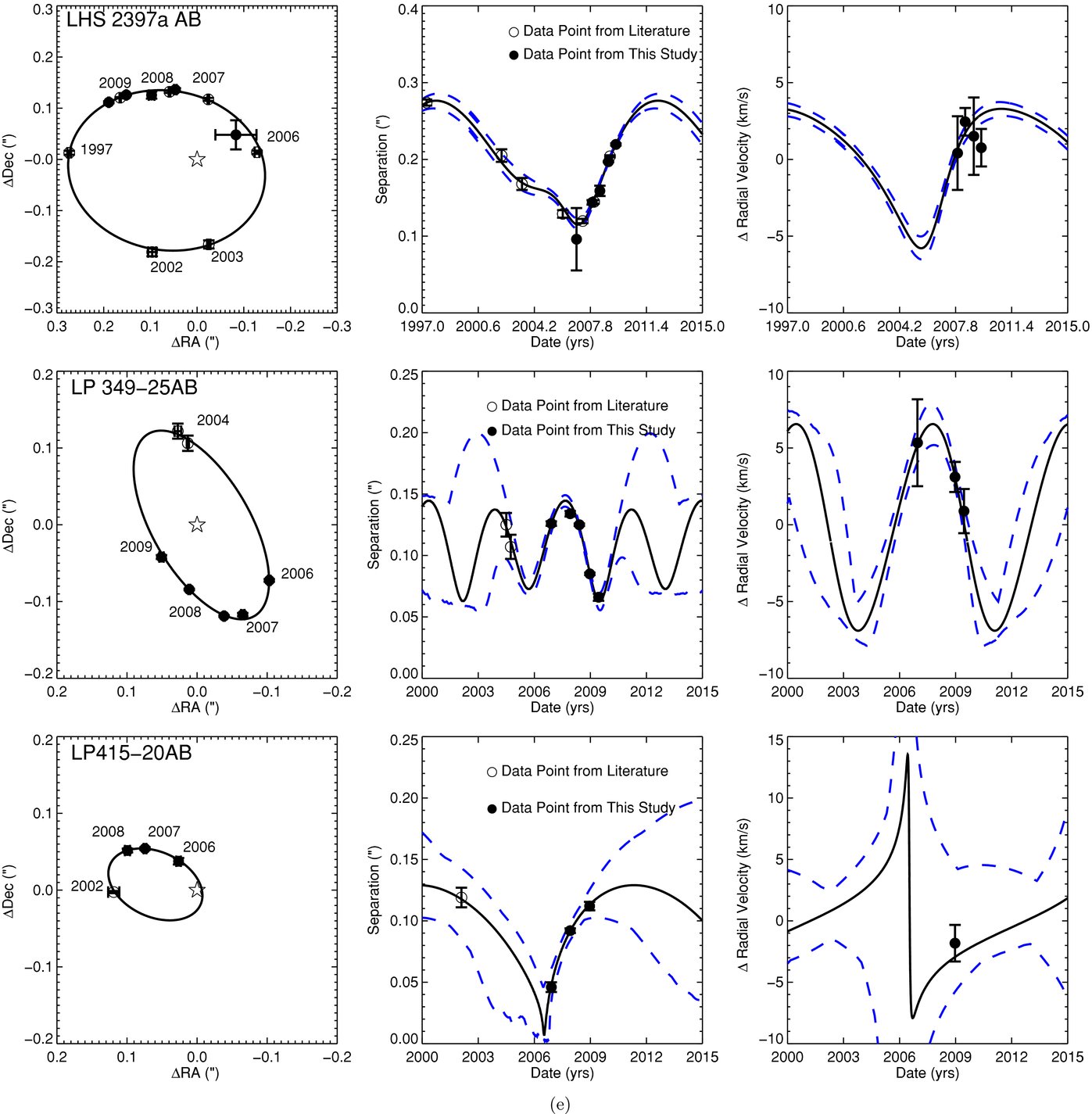
Figure 20. Probability of eclipse as a function of date of occurrence for 2MASS 0920+35 AB. Overall, the system has a 6.8% chance of being an eclipsing system, with the most likely date of eclipse having occurred in 2009 April. The next most likely date of an eclipse is in mid-2012.
Download figure:
Standard image High-resolution image
9. CONCLUSIONS
We have calculated relative orbital solutions for 15 VLM binary systems, using a combination of astrometric and radial velocity data obtained with the Keck Observatory LGS AO system. For ten of these systems, this is the first derivation of the relative orbits, one of which gives the most precise mass yet measured for a brown dwarf binary. We have also calculated the absolute orbital solutions for six systems, five of which are the first for those systems, representing the first individual component masses for several L dwarfs.
The masses we have calculated based on these orbital solutions and our derived temperatures have allowed us to perform the first comprehensive comparison of a sample of VLM objects to theoretical evolutionary models. All systems with mass precision better than 60% show discrepancies with the predictions of evolutionary models. We find that for six systems, their total system masses are underpredicted by both evolutionary models considered. In these systems, 11 of the 12 components have spectral types earlier than L4. We find that one binary T dwarf has its total system mass overpredicted by the evolutionary models. We postulate that for those systems in which we see a discrepancy, the possible cause is either an incorrect radius prediction by the evolutionary models, an incorrect temperature prediction by the evolutionary models, or an incorrect temperature prediction by the atmospheric models.
Future work that would illuminate the apparent mass discrepancies include (1) improving the precision of the dynamical masses, with a particular emphasis on obtaining more individual masses across a broader range of spectral types and (2) obtaining radius measurements for our sources, which we can potentially pursue through the calculation of surface gravity (which, with individual mass, provides a means for calculating radius), or measure directly if 2MASS 0920+35AB is eclipsing. Such measurements will allow us to test the evolutionary and atmospheric models independently.
The authors thank observing assistants Joel Aycock, Heather Hershley, Carolyn Parker, Gary Puniwai, Julie Rivera, Chuck Sorenson, Terry Stickel, and Cynthia Wilburn, and support astronomers Randy Campbell, Al Conrad, Jim Lyke, and Hien Tran for their help in obtaining the observations. We thank Jessica Lu, Tuan Do, Sylvana Yelda, Marshall Perrin, and Will Clarkson for helpful discussions of this work. We also thank an anonymous referee for helpful suggestions for the improvement of this document. Support for this work was provided by the NASA Astrobiology Institute, the Packard Foundation, and the NSF Science & Technology Center for AO, managed by UCSC (AST-9876783). Portions of this work were performed under the auspices of the U.S. Department of Energy by the Lawrence Livermore National Laboratory under Contract DE-AC52-07NA27344. Q.M.K. acknowledges support from the NASA Graduate Student Research Program (NNG05-GM05H) through JPL and the UCLA Dissertation Year Fellowship Program. This publication makes use of data products from the 2MASS, which is a joint project of the University of Massachusetts and the Infrared Processing and Analysis Center/California Institute of Technology, funded by the National Aeronautics and Space Administration and the National Science Foundation. The W. M. Keck Observatory is operated as a scientific partnership among the California Institute of Technology, the University of California and the National Aeronautics and Space Administration. The Observatory was made possible by the generous financial support of the W. M. Keck Foundation. The authors also recognize and acknowledge the very significant cultural role and reverence that the summit of Mauna Kea has always had within the indigenous Hawaiian community. We are most fortunate to have the opportunity to conduct observations from this mountain.
Footnotes
- 10
Though the official publication of Burgasser et al. (2007) in the Protostars and Planets V Conference Proceedings was in 2007, the article was published on astro-ph in 2006 February.
- 11
- 12
- 13
While this method has been shown to produce reliable radial velocities, the V sin i's have known systematics that are perhaps due to an additional degeneracy with the instrumental PSF.
- 14
In contrast to Konopacky et al. (2007), we are not obtaining temperatures based upon the color of our systems. The atmospheric model fits are only linked to bolometric luminosity through the K-band magnitude, and thus the correlations between the two parameters are very weak in this study.
- 15
Since only one system has a spectral type later than L5, we do not perform this exercise for the COND models.