


ABSTRACT
Understanding the connection between the magnetic configurations of a coronal mass ejection (CME) and their counterpart in the interplanetary medium is very important in terms of space weather predictions. Our previous findings indicate that the orientation of a halo CME elongation may correspond to the orientation of the underlying flux rope. Here we further explore these preliminary results by comparing orientation angles of elongated LASCO CMEs, both full and partial halos, to the EUV Imaging Telescope post-eruption arcades (PEAs). By analyzing a sample of 100 events, we found that the overwhelming majority of CMEs are elongated in the direction of the axial field of PEAs. During their evolution, CMEs appear to rotate by about 10° for most of the events (70%) with about 30°–50° for some events, and the corresponding time profiles display regular and gradual changes. It seems that there is a slight preference for the CMEs to rotate toward the solar equator and heliospheric current sheet (59% of the cases). We suggest that the rotation of the ejecta may be due to the presence of a heliospheric magnetic field, and it could shed light on the problems related to connecting solar surface phenomena to their interplanetary counterparts.
Export citation and abstract BibTeX RIS
1. INTRODUCTION
The occurrence of geomagnetic storms is well associated with Earth-directed coronal mass ejections (CMEs), which appear in coronagraph images as bright halos around the Sun (halo CME; Howard et al. 1982). CMEs are eruptions of the solar magnetic field and plasma into interplanetary space, which occur following a large-scale magnetic rearrangement in the solar atmosphere (Zhang et al. 2003; Crooker & Horbury 2006; Gopalswamy et al. 2006; Schwenn et al. 2006). Potential magnetic field modeling (Luhmann et al. 1998, 2003; Zhao & Webb 2003) suggests that the origin of CMEs is global and is related to helmet streamer configurations which are sensitive to the stability of the active regions and/or filaments spanned by the streamers. Depending upon the orientation of the magnetic field in the CME-originating region and the sign of magnetic helicity, the Earth-directed CME may, or may not, have an intense southward Bz field (Yurchyshyn et al. 2001). Hence, the origin of CMEs, the structure of their source regions, and their signatures in the solar wind near the Earth are of fundamental interest in the physics of the Sun, space plasmas, and space weather research.
Interplanetary counterparts of CMEs are called interplanetary CMEs (ICMEs). Those ICMEs that encounter the Earth are usually observed either as complex ejecta or magnetic clouds (MCs). For a number of years now researchers have been trying to establish the relationship between CMEs, their solar progenitors and interplanetary ejecta (see, for example, Gopalswamy 2008a). Since the complex ejecta (Burlaga et al. 1981) represent unorganized and compound magnetic structures, they were not the subject of these studies. Instead, effort was focused on MCs (Burlaga et al. 1981) that generally exhibit a magnetically organized geometry, which is thought to correspond globally to a curved flux rope (Bothmer & Schwenn 1998; Marubashi 2000; Riley et al. 2006) and can be related to the corresponding solar parameters (Crooker & Horbury 2006; Gopalswamy 2008b). In particular, significant research effort was devoted to finding whether the direction of the magnetic field and the sense of twist found in MCs correspond to those in CME source regions (which include both active region and filaments).
According to various case and statistical studies many interplanetary ejecta maintain nearly the same orientation and twist as the source regions they are associated with (Marubashi 1986; Rust & Kumar 1996; Bothmer & Schwenn 1998; Zhao & Hoeksema 1998; McAllister & Martin 2000; Yurchyshyn et al. 2001, 2005a, 2006; Leamon et al. 2002; Ruzmaikin et al. 2003; Ishibashi & Marubashi 2004; Gopalswamy et al. 2005; Hu et al. 2005; Rust et al. 2005; Krall et al. 2006; Wang et al. 2006; Qiu et al. 2007; Yurchyshyn 2008). Several statistical studies, however, produced inconclusive results (Leamon et al. 2002; Wang et al. 2006): while many events show satisfactory agreement between solar and interplanetary fields, there always are outliers, which do not fit the common pattern.
Yurchyshyn et al. (2007) compared orientations of 25 halo CMEs to the corresponding parameters determined for MCs. In this study, CME orientation angles (or tilt) were determined by fitting an ellipse to an irregularly shaped "halo" around the C3 occulting disk and measuring its tilt in the clockwise (CW) direction from the positive Geocentric Solar Ecliptic (GSE) y-axis (roughly corresponding to solar east) to the ellipse semimajor axis. The fitted white-light-propagating structure is thought to represent a shock often associated with CMEs. The main conclusion drawn from this study was that for about 64% of CME–MC events, there is a good correspondence between their orientation angles, which supports the idea that the semimajor axis of an ellipse-shaped halo CME may indeed reflect the underlying structure of the erupting magnetic fields. This was later confirmed by X. P. Zhao (2007, private communication). If this is true, then these results also imply that the majority of interplanetary ejecta do not significantly change their orientations (less than 45° rotation) while traveling from the Sun to the near Earth environment. At the same time, this somewhat weak correspondence between CME and MC orientations seems to reflect the existing general confusion about the relationship between solar and MC fields: while for the majority of events magnetic fields at the Sun and 1 AU seem to be in agreement, a non-negligible minority displays quite different behavior.
Therefore, the question about the magnetic connection between interplanetary ejecta and solar surface phenomena is still not well understood. Hence, no well-defined scheme exists to predict the magnetic field structure at 1 AU based on solar surface measurements. Here we will further explore this problem by utilizing magnetic field information derived from EUV Imaging Telescope (EIT) post-eruption arcades, coronal magnetic field maps, and halo CMEs.
2. CME ORIENTATION AND DIRECTION OF THE AXIAL FIELD IN POST-ERUPTION ARCADES
The event list that we used for this study was originally presented in Tripathi et al. (2004), who analyzed association between 236 PEAs and the corresponding CMEs. For each PEA event, the authors determined its heliographic position and length along the axis, which was generally the overlying magnetic polarity inversion line. The heliographic length of the PEAs was found to be in the range of 2°–40°, with an average of 15°. Because we are interested in exploring the details of the PEA structure, we discarded all narrow and limb CMEs, so that the final list includes 101 PEA–CME events (Table 1). Figure 1 shows the distribution of the selected events on the solar disk with nearly half of the sample originated near the disk center, i.e., at angular distances not exceeding 30° (indicated by a circle in Figure 1).
Figure 1. Distribution of CME source regions on the solar disk. Open/closed circles represent full/partial halos. The 30° circle encloses the disk center halo events.
Download figure:
Standard image High-resolution imageTable 1. List of Full and Partial Halo CMEs
| Event Number | Date | Time (UT) | Location | CME Orientation (deg) | CME Orientation (rms) | PEA Orientation (deg) | Rotation Rate (deg hr−1) | Rotation Rate (rms) |
|---|---|---|---|---|---|---|---|---|
| 1 | 1997 Feb 7 | 04:15:00 | S37W28 | 169.1 | 11.4 | 137.2 | −0.1 | 1.3 |
| 2 | 1997 Apr 7 | 15:33:00 | S29E20 | 139.4 | 59.5 | 136.5 | −18.8 | 8.0 |
| 3 | 1997 May 12 | 08:06:00 | N22W08 | 8.4 | 3.0 | 78.5 | −0.6 | 0.2 |
| 4 | 1997 Aug 30 | 04:01:59 | N30E12 | 240.6 | 23.7 | 145.3 | 5.9 | 3.7 |
| 5 | 1997 Oct 21 | 20:44:00 | N17E05 | 319.3 | 2.9 | 394.6 | −0.3 | 0.0 |
| 6 | 1997 Oct 23 | 14:56:59 | N22E09 | 342.9 | 3.8 | 359.2 | −0.2 | 0.5 |
| 7 | 1997 Dec 6 | 15:36:00 | N28W42 | 127.4 | 79.1 | 40.4 | 21.6 | 6.4 |
| 8 | 1998 Jan 3 | 06:48:59 | N27W39 | 33.7 | 70.5 | 37.3 | −2.7 | 7.2 |
| 9 | 1998 Jan 25 | 17:58:00 | N24E26 | 49.6 | 52.7 | 34 | 0.8 | 1.2 |
| 10 | 1998 Apr 20 | 11:48:00 | S28W84 | 19.7 | 5.2 | 61.5 | 5.4 | 0.8 |
| 11 | 1998 Apr 27 | 11:44:00 | S17E51 | 224.8 | 10.8 | 240.6 | 2.9 | 0.4 |
| 12 | 1998 Apr 29 | 18:38:59 | S15E20 | 240.8 | 66.3 | 211.9 | −25.3 | 11.2 |
| 13 | 1998 May 6 | 10:45:00 | S16W72 | 158.2 | 3.7 | 83.5 | −0.1 | 0.4 |
| 14 | 1998 Nov 2 | 17:29:00 | S33E42 | 158.3 | 3.6 | 89.9 | 2.2 | 0.1 |
| 15 | 1998 Nov 4 | 11:27:59 | N26W02 | 94.2 | 21.2 | 44.6 | 6.9 | 1.9 |
| 16 | 1998 Nov 5 | 00:29:00 | N23W20 | 150.5 | 5.9 | 162.1 | −5.9 | 0.8 |
| 17 | 1998 Nov 9 | 20:29:00 | N18W00 | 77 | 85.3 | 24.9 | −31.2 | 46.4 |
| 18 | 1998 Dec 18 | 18:44:00 | N28E36 | 28.8 | 10.9 | 79.1 | −7.6 | 1.6 |
| 19 | 1999 Apr 4 | 06:18:00 | N13E67 | 146.8 | 63.8 | 4.1 | −37.7 | 14.6 |
| 20 | 1999 Apr 18 | 11:17:00 | N16W04 | 25 | 4.5 | 46 | 3.1 | 3.1 |
| 21 | 1999 May 3 | 06:41:00 | N20E43 | 328.4 | 62.3 | 295.3 | −41.5 | 12.8 |
| 22 | 1999 May 10 | 08:17:00 | N29E51 | 194.2 | 5.4 | 202.5 | −2.2 | 0.5 |
| 23 | 1999 Jun 22 | 20:38:59 | N25E39 | 40.6 | 7.7 | 51.1 | −3.9 | 5.1 |
| 24 | 1999 Jun 24 | 14:40:00 | N31W08 | 80.8 | 30.4 | 37.3 | 10.8 | 9.9 |
| 25 | 1999 Jul 7 | 20:40:59 | N22W50 | 206.8 | 7.3 | 216.8 | −3.1 | 1.8 |
| 26 | 1999 Jul 25 | 14:40:00 | N39W75 | 209.6 | 7.1 | 265 | 1.3 | 1.7 |
| 27 | 1999 Aug 17 | 18:40:59 | N22E38 | 42.3 | 12.7 | 97.4 | 9.1 | 1.3 |
| 28 | 1999 Aug 28 | 20:40:59 | S32W12 | 113.8 | 82.9 | 151.6 | −61.6 | 14.5 |
| 29 | 1999 Sep 12 | 03:14:00 | S14W41 | 70.5 | 6.8 | 136 | 0.7 | 1.1 |
| 30 | 1999 Nov 16 | 08:15:59 | N10W35 | 32 | 1.8 | 36.8 | −0.5 | 0.4 |
| 31 | 1999 Dec 22 | 04:39:59 | N35E30 | 34.6 | 22.8 | 88.8 | −5.7 | 3.3 |
| 32 | 2000 Jan 18 | 20:15:59 | S20E08 | 236.9 | 10.5 | 334.6 | −6.1 | 1.4 |
| 33 | 2000 Feb 8 | 10:41:00 | N22E29 | 260.8 | 67.8 | 337 | 28.3 | 4.9 |
| 34 | 2000 Feb 9 | 20:39:59 | S16W37 | 78.8 | 5.4 | 137.2 | −3.5 | 0.6 |
| 35 | 2000 Feb 17 | 21:39:59 | S29E07 | 97.6 | 32.8 | 63.7 | 37.3 | 3.8 |
| 36 | 2000 Apr 4 | 17:16:59 | N18W58 | 51.6 | 6.5 | 81.8 | −10.9 | 0.7 |
| 37 | 2000 Apr 13 | 01:41:00 | S26W34 | 91.6 | 94.0 | 146.5 | −56.6 | 10.5 |
| 38 | 2000 Jun 6 | 16:16:59 | N19E11 | 93.8 | 8.0 | 42.2 | −4.3 | 1.4 |
| 39 | 2000 Jun 27 | 14:37:59 | N18W68 | 19.8 | 2.5 | 43.7 | 1.7 | 0.6 |
| 40 | 2000 Jun 28 | 20:16:59 | N20W80 | 126.4 | 81.8 | 54.8 | −5.3 | 32.2 |
| 41 | 2000 Jul 7 | 14:17:00 | N13W05 | 68.2 | 6.5 | 89.1 | −5.9 | 1.0 |
| 42 | 2000 Jul 14 | 11:17:00 | N19E00 | 15.9 | 2.1 | 13.7 | −0.7 | 4.1 |
| 43 | 2000 Jul 17 | 10:40:00 | S08E30 | 290 | 11.5 | 296.4 | 6.6 | 2.5 |
| 44 | 2000 Aug 3 | 10:40:00 | N24W71 | 214.5 | 71.3 | 231.6 | −12.4 | 12.5 |
| 45 | 2000 Aug 9 | 17:15:59 | N11W10 | 89 | 32.2 | 77.8 | 14.5 | 3.0 |
| 46 | 2000 Sep 4 | 08:17:00 | N24W32 | 247.1 | 66.6 | 280.1 | 27.3 | 15.4 |
| 47 | 2000 Sep 12 | 12:40:00 | S18W06 | 210 | 8.8 | 142 | 6.4 | 1.6 |
| 48 | 2000 Sep 16 | 05:41:00 | N13W04 | 33.8 | 23.8 | 3.6 | −9.9 | 1.8 |
| 49 | 2000 Oct 9 | 00:41:00 | N00W13 | 311.6 | 9.5 | 333.1 | −1.4 | 1.6 |
| 50 | 2000 Oct 25 | 11:17:00 | N09W53 | 38.7 | 14.6 | 39 | 5.7 | 2.1 |
| 51 | 2000 Nov 1 | 18:16:59 | S13E32 | 113.8 | 8.9 | 159.5 | −5.1 | 0.6 |
| 52 | 2000 Nov 2 | 20:40:59 | N24W56 | 103.4 | 14.9 | 30.5 | 11.2 | 2.6 |
| 53 | 2000 Nov 3 | 23:40:59 | N05E01 | 52.2 | 16.2 | 138.3 | 0.2 | 1.2 |
| 54 | 2000 Nov 16 | 00:39:00 | S24E35 | 283.9 | 7.4 | 281.1 | 3.4 | 0.4 |
| 55 | 2000 Nov 26 | 18:15:59 | S24W48 | 126.6 | 60.1 | 137.2 | −9.2 | 13.1 |
| 56 | 2001 Jan 10 | 02:41:00 | N14E37 | 95.5 | 5.6 | 46.7 | 0.9 | 0.4 |
| 57 | 2001 Jan 20 | 20:16:59 | S05E40 | 35.9 | 14.5 | 86.9 | 9.7 | 1.8 |
| 58 | 2001 Feb 2 | 21:40:59 | N21E55 | 25.6 | 6.6 | 26.9 | −6 | 0.8 |
| 59 | 2001 Feb 28 | 17:40:59 | S13W07 | 316.2 | 10.4 | 238.2 | −1.9 | 1.4 |
| 60 | 2001 Mar 16 | 06:16:59 | N12W11 | 34.6 | 6.6 | 41.1 | 0 | 0.5 |
| 61 | 2001 Apr 5 | 17:40:59 | S21E55 | 265.5 | 12.9 | 330.5 | −7.1 | 2.7 |
| 62 | 2001 Apr 9 | 03:15:00 | S24E09 | 94.6 | 21.4 | 125.1 | 1.2 | 2.2 |
| 63 | 2001 Apr 9 | 16:37:59 | S21W05 | 309.7 | 14.2 | 240.5 | −5.8 | 7.3 |
| 64 | 2001 Apr 10 | 06:13:59 | S23W04 | 99.5 | 23.0 | 102.2 | −31.1 | 7.1 |
| 65 | 2001 Apr 26 | 14:15:00 | N23W07 | 81.4 | 8.9 | 40.5 | −4.7 | 2.1 |
| 66 | 2001 Aug 14 | 16:37:00 | N21W21 | 33.3 | 8.7 | 42.5 | 5 | 0.4 |
| 67 | 2001 Aug 25 | 17:40:59 | S22E35 | 272.5 | 48.0 | 249.2 | −27.6 | 1.2 |
| 68 | 2001 Sep 24 | 11:17:00 | S21E26 | 55.7 | 8.6 | 130.9 | 6.5 | 1.3 |
| 69 | 2001 Sep 28 | 09:38:59 | N09E18 | 287.1 | 69.1 | 292.9 | 17.5 | 15.0 |
| 70 | 2001 Oct 9 | 12:12:59 | S29E05 | 291.4 | 58.4 | 341.5 | −7.1 | 7.9 |
| 71 | 2001 Oct 19 | 18:16:59 | N10W20 | 48 | 16.2 | 82.7 | −4.7 | 1.5 |
| 72 | 2001 Oct 22 | 16:16:59 | S19E20 | 129.8 | 14.5 | 141.8 | 10.3 | 1.6 |
| 73 | 2001 Nov 17 | 06:16:59 | S07E45 | 280.8 | 15.0 | 334.8 | 12.6 | 4.2 |
| 74 | 2001 Nov 22 | 22:15:59 | S24W64 | 239 | 44.0 | 326 | −62.3 | 0.0 |
| 75 | 2001 Nov 23 | 23:40:59 | S19W30 | 207.2 | 8.3 | 271.2 | −0.5 | 0.3 |
| 76 | 2001 Dec 20 | 03:14:00 | S37W19 | 310.5 | 22.1 | 333.8 | −17.4 | 6.9 |
| 77 | 2001 Dec 28 | 21:15:59 | S27E82 | 237.6 | 6.1 | 262 | 0.8 | 0.7 |
| 78 | 2002 Jan 28 | 15:15:00 | S32E23 | 140.9 | 9.2 | 154.2 | 2 | 1.3 |
| 79 | 2002 Feb 12 | 21:17:59 | N10E39 | 381.6 | 5.1 | 359.4 | −4.2 | 1.5 |
| 80 | 2002 Mar 16 | 00:40:00 | S06W09 | 129.7 | 10.2 | 122.3 | −1.9 | 1.5 |
| 81 | 2002 Mar 18 | 04:15:00 | S08W24 | 89.3 | 13.5 | 70.6 | 6.2 | 4.6 |
| 82 | 2002 Apr 15 | 04:41:00 | S15W05 | 38.2 | 11.1 | 138.6 | −5.4 | 2.5 |
| 83 | 2002 Apr 17 | 09:17:00 | S12W35 | 136.7 | 39.2 | 137.2 | −10.9 | 10.4 |
| 84 | 2002 Apr 21 | 02:15:59 | S13W80 | 101.2 | 82.9 | 133 | −50.4 | 23 |
| 85 | 2002 May 22 | 02:16:59 | S20W74 | 83.8 | 61.1 | 114.7 | −57.2 | 7.0 |
| 86 | 2002 May 22 | 04:41:00 | S21W52 | 388.1 | 22.9 | 306.6 | 18.2 | 5.1 |
| 87 | 2002 May 27 | 14:41:00 | N24E16 | 295.2 | 7.3 | 234 | 0.7 | 2.8 |
| 88 | 2002 Jul 15 | 22:16:59 | N27E04 | 48.5 | 10.9 | 78.8 | −5.9 | 1.0 |
| 89 | 2002 Jul 29 | 15:17:00 | S11W15 | 305.9 | 10.5 | 318.2 | 1.1 | 1.0 |
| 90 | 2002 Aug 16 | 14:15:00 | S16E19 | 108.6 | 20.5 | 101.8 | 33.7 | 4.2 |
| 91 | 2002 Sep 5 | 17:39:59 | N05E27 | 62.1 | 89.6 | 118.9 | 41.4 | 38.1 |
| 92 | 2002 Nov 9 | 14:41:00 | S12W27 | 53.5 | 13.8 | 107.2 | −13.7 | 2.4 |
| 93 | 2002 Nov 10 | 03:41:00 | S13W36 | 48.3 | 8.0 | 110.8 | −1.2 | 0.7 |
| 94 | 2002 Nov 24 | 21:16:59 | N18E38 | 284.1 | 16.5 | 235.1 | 11.8 | 4.1 |
| 95 | 2002 Dec 19 | 23:40:59 | N18W09 | 138.1 | 74.5 | 86.4 | −1 | 18.8 |
| 96 | 2003 Mar 18 | 14:17:00 | S14W49 | 111.6 | 68.6 | 131.8 | −40.5 | 13.2 |
| 97 | 2003 Aug 14 | 00:41:00 | N23W02 | 111.3 | 4.6 | 94.4 | 2.6 | 0.8 |
| 98 | 2003 Oct 28 | 11:41:00 | S16E06 | 230.6 | 12.6 | 209.4 | 9.7 | 23 |
| 99 | 2003 Oct 29 | 21:40:59 | S20W06 | 91 | 12.3 | 71.2 | −29 | 0.0 |
| 100 | 2003 Nov 18 | 09:15:59 | S01E15 | 306.3 | 62.4 | 370.9 | −36.6 | 17.3 |
| 101 | 2005 May 13 | 17:10:59 | N11E10 | 59.3 | 44.4 | 45.1 | −121.5 | 0.0 |
Figure 2 presents the distribution of the events depending on their distance (measured in degree of the heliographic coordinate system) from the global coronal neutral line (CNL) determined at 2.5 solar radii from the Stanford coronal field maps (Hoeksema et al. 1983; Hoeksema 1984). About 2/3 of the events are located close to the CNL (or streamer belt), which agrees with earlier reports (Kahler et al. 1999a; Subramanian et al. 1999). Also, the distribution appears to be of a log-normal type with a well-defined maximum at 20° and a long tail, which suggests that there may not be a characteristic distance between the CME source and the CNL.
Figure 2. Distribution of distances (in deg) from the eruption site to the CNL as determined from the Stanford coronal field maps. About 2/3 of the events are situated in close proximity (<30°) to the neutral line, or in other words, to the coronal streamer belt.
Download figure:
Standard image High-resolution imageTripathi et al.'s (2004) data allowed us to determine the tilt (orientation) of the PEAs relative to the solar east–west line and compare it to that of the associated CMEs. The tilt was measured in degrees in the CW direction starting from the east. We estimated that in most cases the absolute error of measurements of PEA angles was ±20°, although in six events the absolute error was estimated to be as large as 90°. This error was determined from many repeating measurements of the PEA angles. Since a PEA is an organized magnetic structure, it has a well-defined axial magnetic field; therefore, we can assign the direction to the PEA orientation angles. The axial field and the direction of twist (helicity sign) in a PEA may be determined from solar data based on (1) direct calculations of the predominant current helicity (Seehafer 1990; Pevtsov et al. 1994; Abramenko et al. 1996), (2) force-free field modeling, (3) magnetic orientation angles (Song et al. 2006), and (4) visual inspection of the loop pattern seen in chromospheric and coronal images such as S- and Z-shaped sigmoids (Rust & Kumar 1996; Canfield et al. 1999) and/or dextral and sinistral filaments (Martin 2003).
CME orientations were determined by fitting an ellipse to an irregularly shaped "halo" around the occulting disk (Yurchyshyn et al. 2007) using L1 level LASCO C3 data (Morrill et al. 2006). Eight points, evenly spaced in the position angle, were measured along the outer edge of the halo in each image available for a given event. At each angle, the edge of the halo is chosen to be the outermost point on the overall expanding CME structure. The measured points were then fitted with an ellipse, and its tilt angle, αCME, was measured in the CW direction from the positive y-axis. To estimate the error of an individual measurement, two researchers independently defined the position of the eight points in the same image. This procedure was repeated for 20 times and the standard deviation of these measurements was found to be 2 6, which we accept as an error of each individual measurement of CME orientation. To compare the CME orientation angles to those of PEAs, we needed to resolve 180° ambiguity in the measured CME angles. It was done by assuming that the direction of the axial field and twist of a flux rope CME corresponds to those of the EIT/Hα flare arcade associated with the eruption. We required that the axial field of the PEA makes an acute angle with that of the CME. We would like to emphasize that the disambiguation process itself does not automatically ensure a good correlation between the two parameters. While their difference may not exceed 90° they might still be poorly correlated and large scatter of data points may be present.
In Figure 3, we plot the CME directional angles versus those of PEAs. The panels represent (from left to right) disk halo CMEs, off-disk halo CMEs, and partial CMEs. First of all, it is worth noting that in all three cases the data points are mainly focused near the bisector: for approximately 58% out of 101 events the difference angle is less than 45°. This ratio is higher (65%) for disk halo CMEs (20 out of 32 events). Figure 3 thus supports our previous reports that, on average, the elongated halos are oriented along the axis of the corresponding EIT post-eruption arcades (Yurchyshyn 2008) and that the ellipse-shaped halo CMEs may indeed bear information on the geometry of the underlying flux rope.

Figure 3. CME orientations plotted vs. those of PEAs. The plots are (from left to right) for disk halo CMEs that originated within a 30° circle centered at the disk center (see Figure 1), off-disk halo CMEs, and partial CMEs. Black (gray) symbols represent events launched from southern (northern) hemisphere. The partial halo events are plotted with pie segments, whose orientation indicates the solar disk quadrant where they originated. The horizontal error bars are standard deviations of measurements associated with each CME event. Vertical error bars represent the absolute error of measurements of PEA orientations, which is accepted for all events to be 20°. The solid line is a bisector and the two dashed lines indicate a 45° range relative to the bisector.
Download figure:
Standard image High-resolution image3. TIME PROFILES OF CME ORIENTATIONS AS MEASURED FROM LASCO IMAGES
In Figure 4, we show a sample of typical CME orientation time profiles. The horizontal axis there represents time, and the vertical axis is the CME orientation angle measured clockwise from the solar east (0° and 90° correspond to solar east and north, accordingly) and the error of individual measurement is smaller than the size of plotting symbols. On average, about half of the events in the data set display clear and gradual changes in their orientation profiles (left panels), while data points for other events are more scattered, so that the time profiles are not gradual (right panels). As it follows from the figure, the total change in the orientation is relatively small: in 70% of cases it does not exceed 10°, although in some cases data show up to 50°–60° change. Figure 5 shows two LASCO C3 difference images for the 2000 September 16 event, and the corresponding time profile is shown in the left column of Figure 4. The halo structures in these two LASCO images were fitted with an ellipse, and it is evident that the orientation of this CME has changed. The CME shape and orientation were mainly determined by the bright core early in the eruption (06:18 UT), which was later superseded by a faint halo at 09:42 UT.
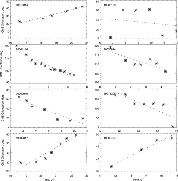
Figure 4. CME orientation time profiles. Each data point represents the orientation angle measured clockwise from the solar east from one LASCO C3 image. The size of the plotting symbol exceeds the absolute error of measurement. Nearly half of the events in our pool display gradual rotation, while data points for the other half are scattered, so that the trend is less prominent but nevertheless present.
Download figure:
Standard image High-resolution image
Figure 5. LASCO C3 images for the 2000 September 16 event. They illustrate the regular rotation of the white-light structure of the CME outlines by the white ellipses.
Download figure:
Standard image High-resolution imageTo probe whether there is any preferable direction of this apparent rotation, we introduced the rotation-rate parameter, which was determined as follows. First, we calculated the angle difference between an ellipse-shaped white-light CME structure in each LASCO C3 frame and the solar equator. We will call this difference the angular distance of the CME from the solar equator. Second, we calculated a derivative of the angular distance time profile, i.e., the rotation rate. The derivative was calculated by fitting the orientation time profile with a line, which also provided a 1σ uncertainty of the fit (see the last two columns in Table 1). Negative/positive rotation rate indicates rotation toward/away from the solar equator, while its magnitude gives us the rotation speed in terms of degree per hour. We chose the solar equator as a reference line because it approximately represents the magnetic equator and the heliospheric current sheet. We most certainly recognize that the heliospheric current sheet is a wavy, complex, and ever changing three-dimensional structure and substituting it with a plane is a gross simplification; however, our current intention is to see if there is any regular pattern in changes of CME orientations.
Figure 6 shows distributions of the rotation rate for all events and for all full halos originating within 30° of the disk center. Both distributions are somewhat asymmetrical relative to zero, with a detectable bulge on the negative side. A simple Gaussian fitting shows that the distributions are centered near x = −3.4 deg hr−1 and 58% of all events (59 out of 101) have negative rotation rate, i.e., 59 events seem to rotate toward the equator during their evolution. This percentage appears to be higher in the case of the disk center full halo CMEs: 69% or 22 events out of 32. We also calculated the average magnitude of the rotation rate separately determined for events with negative and positive rates. In both distributions, the average negative rate of −15 deg hr−1 exceeds the average positive rate of 10 deg hr−1. This suggests that the CMEs with negative rotation rate may rotate faster than those with positive one. We repeated these calculations by discarding all events with the rotation rate smaller than the corresponding uncertainty of the fit. In this case, there were 57% of event with negative rate (44 out of 78 events) and the average negative rate of −15 deg hr−1 exceeded the average positive rate of 7 deg hr−1. We also discarded events with small rotation rate using threshold of 10 deg hr−1 and 20 deg hr−1 (Table 2). Note that the average uncertainty of the fits listed in the last column of Table 1 is 5.5 deg hr−1 with a standard deviation of 8 deg hr−1. As it follows from Table 2, the ratio of events with negative and positive rotation rates increases when higher threshold is used and so does the average rotation rate.

Figure 6. Distribution of the CME rotation rate (deg hr−1) plotted separately for all events (left panel) and halo CMEs (right panel). The rotation rate was calculated relative to the solar equator. Negative/positive rotation rate indicates rotation toward/away from the solar equator. The distribution is weakly asymmetrical and centered at x = −3 deg hr−1. There are 61 out of 101 events with negative rotation rate. These events that turn toward the equator, on average, do so faster as compared to ones with positive rotation rate.
Download figure:
Standard image High-resolution imageTable 2. Distribution of Events Depending on Their Rotation Rate (RR) and the Threshold Used
| Threshold (deg hr−1) | Events with Negative RR | Average Negative RR (deg hr−1) | Events with Positive RR | Average Positive RR (deg hr−1) | Event Ratio (%) |
|---|---|---|---|---|---|
| 0 | 59 | −15.9 | 42 | 9.6 | 58 |
| 10 | 21 | −37.8 | 14 | 21.2 | 60 |
| 20 | 15 | −47.3 | 6 | 31.9 | 71 |
Download table as: ASCIITypeset image
Figure 7 shows results similar to those in Figure 6; however, the rotation rate here was determined relative to the CNL as indicated in the relevant Stanford coronal field maps (Hoeksema et al. 1983; Hoeksema 1984) instead of the solar equator. Although the distributions of the rotation rate calculated relative to the CNL and the solar equator appear somewhat different, their parameters are very similar with dominating negative rotation rate.
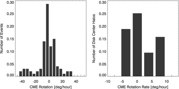
Figure 7. Distribution of the CME rotation rate calculated relative to the CNL as determined from the Stanford coronal field maps. The left (right) panel shows distribution for all (halo) events.
Download figure:
Standard image High-resolution imageOne of the questions which immediately arises and that is relatively easy to address is whether this apparent rotation is in any way associated with CME dynamics. In Figure 8, we show two probability distributions of the rotation rate separately plotted for slow and very fast ejecta. Here, the speed threshold was set to 1200 km s−1. This choice is arbitrary and based on the fact that CMEs with speeds exceeding 1200 km s−1 are relatively rare and often associated with intense geomagnetic storms (Yurchyshyn et al. 2005a, 2005b; Gopalswamy 2008b). These two plots are different and changes in the speed threshold did not result in significant variations of the distributions. As it follows, the bulk of slower ejecta tends to display smaller rotation rates (taller and narrower distribution with a sigma of 6.2 deg hr−1), while the very fast events seems to be more often prone to rotate faster (the distribution is flatter and wider with σ = 12.9 deg hr−1).
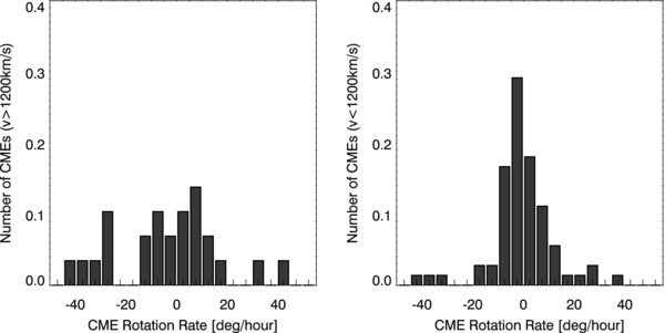
Figure 8. Distribution of the CME rotation rate (deg hr−1) for fast (v > 1200 km s−1, left) and slow (v < 1200 km s−1, right) CMEs.
Download figure:
Standard image High-resolution image4. CONCLUSIONS AND DISCUSSION
First, we would like to briefly summarize the above research.
- 1.We found a good correlation between the orientation of the axial field in EIT post-eruption arcades and that of halo CMEs; this holds true for both full and partial halos.
- 2.Majority of eruptions occurred near the CNL (streamer belt) as determined from the Stanford coronal field maps, while the location of approximately 1/3 of eruptions was more than 30° away from the CNL.
- 3.Most of the CMEs in our data set display gradual changes in their orientation time profiles during their evolution. There seems to be a week tendency (60% of events) for ejecta to have a negative sense of rotation, i.e., toward the solar equator. On average, the rotation rate for the CMEs rotating toward the equator was found to be higher than that for CMEs rotating away from the equator.
- 4.There seems to be a tendency for fast CMEs (v > 1200 km s−1) to display higher rotation rates as compared to slower CMEs.
Rotation of CME structures, reported in this study, may occur for several reasons. First, an operator error during manual measurements could introduce variations in the CME orientation time profiles. Our estimates are that the operator errors are of order of 26. However, they should be random and do not cause gradual changes in the time profile. Nevertheless, analysis of an extended CME data set performed with a robust automated tool is needed in order to confirm these findings.
Another possibility is that this apparent rotation may be caused by variation of intensity of Thompson scattering as the CME moves away from the Sun. Vourlidas & Howard (2006) tested plane-of-the-sky assumption and analyzed brightness of CMEs as seen in a coronagraph, depending on the location of an observer relative to the Sun, and they found that CME brightness remains constant at all heliocentric distances below 50 R☉ and the Thompson scattering should be taken into account only when analyzing heliospheric images such as provided by the STEREO HI instruments (Eyles et al. 2009). However, it should be noted that due to uneven distribution of material and different brightness contrast at the outer and inner edges (relative to the center of the Sun) of the ejecta a bias may be introduced in measurements of the edge of the CME, thus leading to the time dependence of CME orientation. We hope that multipoint data on CME evolution from STEREO and Advanced Composition Explorer (ACE) missions may help to resolve this question.
Apart from possible measurement and instrumental errors mentioned above, the apparent rotation of CMEs could also be due to the evolution of the erupted magnetic fields. Coronal ejecta have a tendency not only to be deflected toward the heliomagnetic equator and channeled into the heliospheric current sheet (HCS; Crooker et al. 1993; Zhao & Hoeksema 1996; Mulligan et al. 1998; Kahler et al. 1999b), but also to be locally aligned with it (Mulligan et al. 1998; Zhao & Hoeksema 1998; Yurchyshyn 2008). These ideas, though, are not always supported by observations (Huttunen et al. 2005; Forsyth et al. 2006).
An example that illustrates the proposed CME rotation is presented in Figure 9. It shows CCMC coronal field model results for Carrington rotation (CR) 2006. The left panels are coronal field maps at 1.6 R☉, while maps at 2.5 R☉ are shown in the right panels. Overplotted ellipses show orientation of the 2003 August 14 CME associated with a weak C3.6 flare in NOAA AR 10431. The orientation of the corresponding MC is indicated by the cylinder over-plotted on the right panels. This CME was relatively slow (∼400 km s−1), associated with the streamer belt and its orientation initially matched the local tilt of the CNL at 1.6 R☉ (thick curve, left panels). However, further out from the Sun the neutral line changed its orientation, which is evident from the 2.6 R☉ map (lower right). It is quite possible that the associated CME rotated too, since the corresponding MC measured at 1 AU was well aligned with the CNL at 2.6 R☉.

Figure 9. Coronal field maps calculated for Carrington rotation 2006 with the potential field solar surface model run at Community Coordinated Model Center. Left panels show maps for source surface radius of 1.6 solar radii; right panels show maps at 2.5 radii. The thick black contour is the CNL. The oval represents the halo CME on 2003 August 14, which was aligned with the CNL at 1.6 solar radii. Magnetic topology has changed further outward from the solar surface so that the neutral line was rotated by approximately 50° and was co-aligned with the MC at 1 AU (cylinder, lower right panel).
Download figure:
Standard image High-resolution image
The rotation of this CME structure was inferred based on measurements of an ejecta-associated shock, instead of the underlying flux rope. It is usually thought that a shock associated with a CME is a three-dimensional shell-like structure enveloping the erupting magnetic fields, which often may have a flux-rope-like structure (see, for example, Vourlidas et al. 2003). Therefore, in our view it is reasonable to assume that a shock, driven by an expanding flux rope, will change it orientation as the underlying flux rope rotates. Based on this speculation and data in Figure 9 we present one possible interpretation of this event.
The black dotted line in the upper left panel approximately indicates the location and shape of the CNL. As it follows from the figure, the erupting flux rope, which was sigmoid shaped, could undergo kink or torus instability, so that the loop top could rotate as it evolves (Török et al. 2004; Green et al. 2007). Thus, the direction of rotation in the 2003 August 14 eruption as well as the preferred rotation of CMEs toward the solar equator qualitatively agrees with findings by Green et al. (2007): this Z-type sigmoid (negative helicity) rotated counterclockwise. Isenberg & Forbes (2007) reported that flux rope rotation may occur due to J × B force that appears when the ejecta's axial field is not aligned with the large-scale overlying magnetic field. The degree and direction of the rotation are governed by the strength of the large-scale field. It is in accord with the Yurchyshyn (2008) report that those ejecta which were not initially aligned with the CNL appear to be rotating so that the resulting MC is locally aligned with the heliospheric current sheet. Also, Lynch et al. (2008, 2009) and Gibson & Fan (2006) proposed that an expanding flux rope can reconnect with the surrounding fields so that the footpoints of the erupting fields can be displaced. The problem with this interpretation is that the rotation of a shock may occur if it is driven by a rotating flux rope and the shock it is coupled to the flux rope, i.e., the CME is accelerating. However, when the CME begins to decelerate, the shock de-couples and it may no longer respond to the rotating CME body. Because the deceleration occurs within the LASCO C3 field of view, the above interpretation may not be valid (at least for part of the events) since for most of time the shock seen in LASCO C3 may be decoupled and thus not driven.
Another equal and/or additional possibility can be that a CME, which was not initially aligned with the heliospheric current sheet, experiences strong interaction with the coronal fields (drag) due to coronal viscosity, which may affect CME speeds (Gopalswamy et al. 2001) and, quite possible, their orientation. The drag is thought to be a quadratic function of CME velocity (Vrsnak et al. 2004), so that faster CMEs may be affected in larger degree. These considerations seem to agree with our data showing faster CMEs to have larger rotation rates. Other solar surface features such as nearby coronal holes may affect the ejecta too (Liu 2007).
Finally, whatever the reason of the rotation may be, the present analysis suggests that the rotation of CMEs may play an important role in the present confusion in the understanding of the magnetic connection between the interplanetary ejecta and their corresponding solar surface phenomena. Therefore, a rotation of the CME structure should be taken into account while attempting to make a correlation between the CME source region configuration and their interplanetary counterparts.
We thank the referee for careful reading of the manuscript and valuable suggestions and criticism that led to significant improvement of the paper. The CME catalog is generated and maintained by the Center for Solar Physics and Space Weather, the Catholic University of America in cooperation with the Naval Research Laboratory, and NASA. We acknowledge the usage of the list of geomagnetic storms compiled during a Living With a Star Coordinated Data Analysis Workshops. SOHO is a project of international cooperation between ESA and NASA. We thank A. Vourlidas for fruitful discussions and assistance in obtaining LASCO C3 level 1 data. The authors also thank B. Kliem and LWS TR&T focus team "Interplanetary magnetic fields" for insightful discussion. V.Y.'s work was supported under NASA's GI NNX08AJ20G and LWS TR&T NNG0-5GN34G grants.