


ABSTRACT
A study of the magnetic configuration and evolution of a long-lasting quiescent coronal sigmoid is presented. The sigmoid was observed by Hinode/XRT and Transition Region and Coronal Explorer (TRACE) between 2007 February 6 and 12 when it finally erupted. We construct nonlinear force-free field models for several observations during this period, using the flux-rope insertion method. The high spatial and temporal resolution of the X-Ray Telescope (XRT) allows us to finely select best-fit models that match the observations. The modeling shows that a highly sheared field, consisting of a weakly twisted flux rope embedded in a potential field, very well describes the structure of the X-ray sigmoid. The flux rope reaches a stable equilibrium, but its axial flux is close to the stability limit of about 5 × 10²⁰ Mx. The relative magnetic helicity increases with time from February 8 until just prior to the eruption on February 12. We study the spatial distribution of the torsion parameter α in the vicinity of the flux rope, and find that it has a hollow-core distribution, i.e., electric currents are concentrated in a current layer at the boundary between the flux rope and its surroundings. The current layer is located near the bald patch separatrix surface (BPSS) of the magnetic configuration, and the X-ray emission appears to come from this current layer/BPSS, consistent with the Titov and Démoulin model. We find that the twist angle Φ of the magnetic field increases with time to about 2π just prior to the eruption, but never reaches the value necessary for the kink instability.
Export citation and abstract BibTeX RIS
1. INTRODUCTION
Flares and coronal mass ejections (CMEs) are thought to be due to magnetic eruptions, i.e., the explosive release of magnetic free energy initially stored in a twisted and/or highly sheared, non-potential magnetic field (Priest & Forbes 2002). It has been noted based on images from the Yohkoh soft X-ray telescope (SXT; Tsuneta et al. 1991) that many of these eruptions originate in sinuous structures, usually located near or in active regions (Acton et al. 1992; Moore et al. 2001; Canfield et al. 1999). Canfield et al. (1999, 2007), show that 68% of the erupting active regions have this specific shape before the eruption. Rust & Kumar (1996) call these coronal structures sigmoids. Since most sigmoids are connected to CMEs or flares and these events are of great interest, it is important to understand the magnetic structure of sigmoids prior to eruption.
Sigmoids are generally classified as transient (tens of minutes to hours; Sterling & Hudson 1997; Moore et al. 2001) or long-lasting (days or weeks; Leamon et al. 2003), and appearing in active or quiet regions. All sigmoids have an S- or inverse-S shape with two elbows curved in opposite directions. Sigmoids are located above polarity inversion lines (PILs) in the photosphere. Usually, one elbow is rooted in the positive magnetic polarity and the other in the negative polarity, while in the middle of the sigmoid the loops are aligned with the PIL. It is now known that sigmoids are composed of multiple loops that run low and parallel to the central part of the sigmoid and curve at the elbows (McKenzie & Canfield 2008). The arms of the elbows come close together in the middle of the sigmoid where they can interact (Moore et al. 2001). Sigmoids are thought to contain highly sheared magnetic fields embedded in envelope fields that are considerably more potential (Moore & Roumeliotis 1992). Canfield et al. (1999, 2007) studied 107 sigmoids in Yohkoh SXT images and found that most of the sigmoids in the Southern hemisphere are S-shaped and composed of right-bearing loops, and those in the North are inverse S-shaped and consist of left-bearing loops (see also Rust & Kumar 1996; Zirker et al. 1997; Pevtsov et al. 2001).
Leamon et al. (2003) measured the twist angles of 191 sigmoidal active regions and reported that most often the twist in these structures is much less than 2π for erupting active regions. They concluded that the kink instability does not play an important role in the eruptions. However, Leamon et al. (2003) estimated the twist based on the best α value from linear force-free models of the whole active regions. According to Leka et al. (2005), this approach yields systematically lower twists and instead one should use the peak α on the axis of the flux rope in order to give a more realistic estimate.
Some active region sigmoids are associated with Hα filaments (Rust & Kumar 1996; Gibson et al. 2002; Pevtsov 2002). Both the filament and the sigmoid lie above the PIL. At least in cases when there is a sigmoid eruption and no significant disruption of the filament, the sigmoid is situated higher in the corona than the filament, and no loops come in between them (Pevtsov 2002). The filament is considered to be supported against gravity in the dips of a twisted flux rope, which is usually invoked to explain the magnetic topology of the filament–sigmoid system (e.g., Rust & Kumar 1994). In this picture, most of the filament lies under the sigmoid. In the case of a transient sigmoid, the standard model of a two-ribbon flare (Shibata 1999) can be employed to explain the existence of sigmoidal loops under the rising filament.
Filaments lie above filament channels in the chromosphere (Gaizauskas 1998), and can be classified as either dextral or sinistral depending on the direction of the magnetic field along the channel as seen from the positive polarity side of the channel (Martin et al. 1992). S-shaped sigmoids are typically associated with sinistral channels and right-helical twist, and inverse-S sigmoids are associated with dextral channels and left-helical twist. Pevtsov et al. (1997) find 90% positive correlation between the orientation of the S and the sign of the helicity. A hemispheric pattern has also been observed for filaments (Leroy 1989; Martin et al. 1994; Martin 1998; Pevtsov et al. 2003).
Several models have been developed to explain the shape of sigmoids and the associated eruptions (Titov & Démoulin 1999; Low & Berger 2003; Kliem et al. 2004; Fan & Gibson 2004; Kusano 2005). For a summarized description of sigmoid models, one can refer to Green et al. (2007). The model by Titov & Démoulin (1999) (referred to as the TD model hereafter) is based on the emergence of a twisted flux tube through the photosphere into an external potential field. A special separatrix surface forms where the field lines touch the polarity inversion line at the so-called bald patch (BP). These lines form a bald patch separatrix surface (BPSS) that separates the flux rope from its surroundings. Subsequently, a current sheet develops at the BPSS, and reconnection occurring at this current sheet can release enough energy to heat the plasma to X-ray temperatures (e.g., Parker 1994). This picture is consistent with a persistent sigmoid. The TD model predicts that a dextral flux rope (with left-handed twist) produces an inverse-S current sheet and a sigmoid, and correspondingly a sinistral flux rope (with right-handed twist) forms an S-shaped sigmoid, consistent with observations. According to this model, the flux rope can remain stable for a long time before it rises enough to develop a kink instability and erupt. After the instability develops, the field lines that graze the photosphere just above the BP are free to lift off, which is consistent with observations of long diffuse clouds lifting off along the axis of the sigmoid. When the field lines detach, the arms of the sigmoid come closer together to fill the vacated space, and this is when a short arcade of loops forms across the PIL. Both of these structures have been observed (e.g., Rust & Kumar 1996; Moore et al. 2001).
Y. Fan and S. Gibson published a series of papers in which they numerically model an emerging flux rope in a potential coronal arcade (Fan & Gibson 2004, 2006, 2007; Gibson & Fan 2006). In some of their models, they obtain that the kink instability plays an important role in the eruption of the flux rope (Fan & Gibson 2004, 2007) and in these cases their models are suitable for describing transient sigmoids that brighten up minutes to hours before the eruption and quickly die out afterward (Sterling & Hudson 1997; Moore et al. 2001). These models predict that when a sufficient amount of magnetic helicity is transported into the corona from the points where the flux tube is anchored in the photosphere, the flux tube writhes and a filamentary current sheet is formed, which appears as the sigmoid. The other case considered in Fan & Gibson (2007) also describes the eruption of a sigmoidal flux rope but as a consequence of the development of a torus instability with much less twist present within the flux rope. Therefore, based on this set of simulations, we can conclude that the presence of a kink instability is not a necessary condition for eruption. The work of Fan & Gibson (2006) and Gibson & Fan (2006) can be regarded as numerical simulations of the analytical TD model since they also demonstrate the existence of the same basic features of this model—the current sheet at the BPSS where extensive heating takes place and facilitates the appearance of a persistent sigmoid.
The question whether the kink instability is important in sigmoid eruptions takes a central place in the discussion of sigmoid models. In our study, we address this question by estimating the twist angle of the sigmoid field lines. An equally important problem for such a discussion is the value of the twist angle at which a kink instability can develop. This value highly depends on the configuration of the flux rope and the ambient coronal field. The value of 2π is often mentioned but it is important to note that this is a too low of a value since it is based on nonline tied magnetic fields which is not the case for the coronal flux ropes. Models of flux ropes in an external field, which is the configuration we use in our models, give values closer to 3.5π for the critical twist (Fan & Gibson 2003, 2004; Török et al. 2004). This value even increases with increasing aspect ratio of the loops involved (Baty 2001; Török et al. 2004).
The study of the structure, evolution, and eruption of sigmoids is made possible by the unprecedented spatial and temporal resolution of the X-Ray Telescope (XRT; Golub et al. 2007) on Hinode. McKenzie & Canfield (2008) observed a long-lasting sigmoid in 2007 February. They found that the Titov & Démoulin (1999) model best matches the observations of this sigmoid. In the present paper, we further analyze the XRT observations of this sigmoid, and we develop nonlinear force-free field (NLFFF) models describing its three-dimensional (3D) magnetic structure.
The purpose of the NLFFF modeling is to determine whether the observed fine structures of the sigmoid can be explained in terms of stable quasi-static models (as suggested by the long lifetime of the sigmoid). We test the hypothesis by Titov & Démoulin (1999) that the most prominent coronal loops are located near a BPSS. We also investigate how electric currents are distributed within the sigmoid, which is important for understanding whether the kink instability plays a significant role in its eruption. A series of NLFFF models covering a seven-day period are constructed. Using these models, we investigate how the parameters of the magnetic configuration (axial and poloidal fluxes, magnetic energies) change in time. The NLFFF models are constructed using the flux-rope insertion method (van Ballegooijen 2004; van Ballegooijen et al. 2007; Bobra et al. 2008; Su et al. 2009). This method involves inserting a weakly twisted flux rope into a potential field and then allowing the field to relax to a force-free state. The models are constrained by the observed shapes of coronal loops seen in the XRT images. For the photospheric boundary conditions, the flux-rope insertion method only requires line-of-sight (LOS) magnetograms (as opposed to extrapolation methods, which require vector magnetograms). The flux-rope insertion method has some limitations that we will discuss, but provides good insight into the three-dimensional magnetic structure of sigmoids.
The paper is organized as follows. In Section 2 we discuss the observations of the sigmoid. We consider the question of how the sigmoid was formed, and whether it evolved into a 2-J or S-shape at its most prominent. We were able to identify single loops from the elbows and arms of the sigmoid that can be used as observational constraints on the NLFFF models. In addition, we use images from the Transition Region and Coronal Explorer (TRACE; Handy et al. 1999) to constrain the position of the flux rope, and full-disk LOS magnetograms from the Michelson Doppler Imager (MDI) on the Solar and Heliospheric Observatory (SOHO; Scherrer et al. 1995) to obtain the radial magnetic field at the photosphere. In Section 3, we describe the modeling, including details of the flux-rope insertion method, the fitting of model parameters to the observations, the magnetic structure of the sigmoid, and its evolution over 7 days. In Section 4, we discuss the distribution of electric currents and the stability of the magnetic configurations. The conclusions are summarized in Section 5.
2. OBSERVATIONS
During the period 2007 February 6–12, Hinode/XRT performed high-resolution (1'') observations of a long-lasting coronal sigmoid (McKenzie & Canfield 2008). Between February 11 06:11 UT and February 12 05:30 UT, the cadence of the images was about 30 s, and the rest of the time the evolution of the sigmoid could be followed using full-disk synoptic images taken every 6 hr. The field of view of the high-cadence images is 384'' × 384''. The primary filter for these observations was the "thin-aluminum/polyimide" (Al/poly) filter, but images taken at lower cadence with the "titanium/polyimide" (Ti/poly) filter were also used. These XRT observations give us an opportunity to study the evolution of the sigmoid's multiple loops. In addition, we obtain MDI full-disk magnetograms (resolution 4'') for the period February 6–12. Figure 1 shows a comparison of XRT images and MDI magnetograms for February 7 and 12.

Figure 1. XRT Ti/poly images (left) and corresponding MDI magnetograms (right). The first set is for February 7, 12:14 UT, and the second one is for February 12, 05:32 UT. The upper magnetogram shows two bipolar regions, and the lower one shows them merged together into one. White is positive polarity, and black is negative.
Download figure:
Standard image High-resolution imageThe MDI data indicate that in the early days of the observation (February 6 and 7) two bipolar regions have come close together but are still separate (see the upper right panel of Figure 1). The regions emerged on the far side of the Sun, so we do not have data on the formation of these regions. In the later days, these two regions seem to merge and form a larger one with a single PIL. Estimates of the magnetic flux in the 384'' × 384'' region on the magnetogram are not conclusive on the issue of flux emergence or cancellation due to high noise levels close to the limb. On the other hand, close inspection of an MDI movie1 encompassing the whole period that the sigmoid region is on the disk shows that there might be some evidence of photospheric flux cancellation. The two separate regions move toward each other along the SE–NW direction, and during this motion the opposite polarity sections of the two regions meet and at this place flux cancellation may take place. This observation is interesting because it has been suggested that magnetic reconnection associated with flux cancellation plays an important role in the formation of flux ropes in the solar atmosphere (e.g., Mackay et al. 2008).
The XRT images from February 6 and 7 show that on these dates the sigmoid is not yet clearly defined. Only the southern region shows evidence for the non-potential structure, while the northern region contains loops that are consistent with a potential field (see upper panels of Figure 1). However, over the course of the next several days the merged region develops a clear S-shape. From February 9 until its eruption on February 12 the sigmoid is remarkably stable. The length of the sigmoid as measured on the XRT images from February 12 is about 182 Mm, and the elbow separation is about 106 Mm.
On most days the sigmoid clearly consists of a collection of S-shaped coronal loops. However, a closer inspection of the XRT images from February 12 indicates that there are faint S-shaped loops together with two J-like structures composed of multiple loops and curved in opposite directions at the elbows. The overlap of the J-shape and the faint S-shape coronal loops creates the impression that the X-ray emission comes from a two-J-like structure which has been proposed by McKenzie & Canfield (2008). From the bottom magnetogram in Figure 1 one can notice two opposite polarity magnetic elements near the bend of the PIL, which most likely are the locations where the J-like loops start. We will explore this issue further when we consider the NLFFF models for this date and time.
Around 6:00 UT on February 12 the first signs of an eruption appear with an onset of a series of large-scale motions. Then a faint diffuse linear structure, almost as long as the sigmoid, appears to lift off from the central part where the two J's come together (McKenzie & Canfield 2008). Around 7:40 UT a low-lying sheared arcade of X-ray loops starts to brighten, which signifies the moment when the X-ray flare begins (see footnote 1). By the end of the next day (February 13), no S-shape remains distinguishable. Similar motions of coronal structures before and during X-ray flares in sigmoids have been reported by other authors (Rust & Kumar 1996; Sterling et al. 2000; Moore et al. 2001).
We utilize images from the Global High-Resolution Hα Network2 to determine whether a filament is present below the sigmoid. A thin filament can be seen in the Hα images from Observatoire de Paris (Meudon), and from Kanzelhöhe Solar Observatory for the period February 7–14. The filament is located above the PIL in the magnetograms. The position of the observed filament provides a constraint on the location and length of the flux rope in the NLFFF models. It is interesting to note that the filament is most prominent on February 11 and 12. Then, it gets disrupted by the eruption of the sigmoid and reappears again on February 13. This can be evidence that the flux rope has only partly erupted at the time of the flare and the remaining part is still able to support a filament. Gibson & Fan (2006) construct a numerical simulation that shows the partial eruption of a flux rope and the formation of post-flare loops after the departure of the erupting part and on top of the remaining part. A large number of observational cases of partly expelled flux ropes have been reported by Pevtsov (2002).
We also use TRACE 171 Å images taken on February 11 and 12 to further constrain the position of the filament. Figure 2 shows that a faint dark filament is visible in the TRACE images from those days. On February 11, the filament seems to be composed of two parts which meet in the middle and on February 12 the filament is one whole structure. At the north-western and south-eastern ends of the filament are regions of bright diffuse "moss" (e.g., Berger et al. 1999), which represents the footpoints of the hot S-shaped coronal loops seen in the XRT images. In addition, TRACE and XRT images from February 12 after the eruption (Figure 3) show the presence of two transient coronal holes at the two ends of the sigmoid. Similar structures have been observed by Zarro et al. (1999). A possible explanation is that coronal material has been evacuated by the eruption (possibly by the lifting off of the long diffuse cloud) and thus lowering the density in the corona on both sides of the sigmoid.

Figure 2. Two TRACE 171 Å images taken on 2007 February 11, 06:41UT (left) and on 2007 February 12, 04:00 UT (right). The field of view is 384'' × 384''. The dark filament as well as some bright coronal loops are clearly visible. On February 11 the filament consists of two parts that nearly touch in the middle of the region, while on February 12 it is one whole filament.
Download figure:
Standard image High-resolution image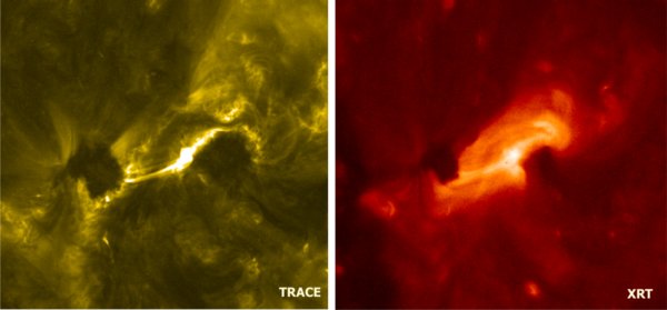
Figure 3. Transient coronal holes at the two ends of the sigmoid. On the left is a TRACE 171 Å images taken on 2007 February 12, 10:05 UT, and on the right an XRT Ti/poly image from the same time.
Download figure:
Standard image High-resolution image3. MODELING THE NON-POTENTIAL MAGNETIC FIELD OF THE CORONAL SIGMOID
As mentioned earlier, a coronal sigmoid contains a highly sheared and/or twisted magnetic field that is embedded in a more potential envelope field (Moore & Roumeliotis 1992). The sheared field can be modeled as a flux rope that is held down by an overlying coronal arcade (e.g., Titov & Démoulin 1999). For long-lasting sigmoids the magnetic field must be in an equilibrium state such that the forces due to the plasma (pressure gradients and gravity) are balanced by the Lorentz force. Most sigmoids lie in regions of the corona where the plasma pressure is small compared to the magnetic pressure (β ≪ 1). Therefore, the Lorentz force must be small, j × B ≈ 0, where B(r) is the magnetic field and j(r) is the electric current density. Using Ampere's law, the force-free condition can also be expressed as a balance between magnetic pressure and tension forces, or by the fact that the electric currents must flow parallel to the field lines: ∇ × B ≈ αB, where α(r) is the so-called torsion parameter. When α = 0 we have a potential field; when α is constant we have a linear force-free field; and when α is a function of position we have a NLFFF. In a NLFFF, α must be constant along field lines (because B · ∇α = 0), but different field lines can have different values of α.
Linear force-free field models cannot accurately describe both the sheared field of the sigmoid and the unsheared field in its surroundings, so we must resort to NLFFF models. Many authors have developed NLFFF models by "extrapolating" vector magnetograms from the photosphere into the corona. For a discussion of these extrapolation methods and various optimization techniques, please refer to Schrijver et al. (2006, 2008), Metcalf et al. (2008) and DeRosa et al. (2009). In the present case, vector magnetograms are not available, so we use a different method in which the NLFFF models are constrained directly by the observed coronal loop structures and only a LOS magnetogram is required. The method involves inserting a coronal flux rope into a potential field model of the active region, and then relaxing the field to a force-free state using magneto-frictional relaxation (van Ballegooijen 2004). The method for constructing the models is described in more detail in the following subsection. In Section 3.2, we describe how the model parameters are fitted to the XRT observations. The results of this fitting are presented in Sections 3.3 and 3.4.
3.1. Flux-rope Insertion Method
To construct three-dimensional magnetic models of the sigmoid, we consider a wedge-shaped domain covering a large area surrounding the sigmoid and extending from the solar surface (r = R☉) to r ≈ 2 R☉. The magnetic field B(r) in the domain is expressed in terms of the vector potential A(r), so that the condition ∇ · B = 0 is automatically satisfied. The numerical computation uses a three-dimensional grid with variable grid spacing, so that the number of cells is minimized while the spatial resolution in the low corona is maximized (Bobra et al. 2008). The cell size on the photosphere is δϕ = 1.5 × 10⁻³R☉ for all models.
The radial component of the magnetic field on the lower boundary, Br(R☉, λ, ϕ) as a function of latitude λ and longitude ϕ, is derived from an MDI magnetogram. We assume that Br = B∥/cos θ, where B∥ is the observed LOS magnetic field and θ is the heliocentric angle. This method is most accurate when the observed photospheric field is radially oriented (as is usually the case outside sunspots), or the object is close to the disk center (so that Br = B∥). The method fails in sunspot penumbrae away from the disk center because penumbral fields are inclined with respect to the radial direction. However, this does not concern us here because the observed active region does not contain sunspots. Once the radial field Br(R☉, λ, ϕ) is known, the potential field Bpot(r) can be computed (for details see the Appendix in van Ballegooijen et al. 2000).
The next step is to specify the parameters of the flux rope, including its path on the solar surface and its axial and poloidal fluxes. The flux-rope path is manually selected. For February 11 and 12, the selection is guided by the observed location of the filament in the TRACE images. The path starts in the positive polarity on one side of the PIL, follows the PIL along the observed filament, and ends on the negative polarity on the other side of the PIL. Figure 4 shows the selected path for February 12, 05:32 UT, overlaid on the longitude–latitude map of the radial field. Note that the selected path has a sinistral orientation compared to the surrounding fields. On the later dates, the path extends along the full length of the PIL of the merged region, but for February 6 and 7 we select a shorter path that extends only along the PIL of the southern-most region (see Figure 1). Other parameters are the axial flux of the flux rope, Φaxi (in Mx), and the poloidal flux per unit length along the flux rope, Fpol (in Mx cm−1). We then modify the surface field Br(R☉, λ, ϕ) by inserting two magnetic sources at the ends of the selected path with fluxes equal ±Φaxi. This modification is necessary to ensure that, upon inserting the flux rope into the three-dimensional model, the original observed flux distribution is recovered.

Figure 4. Selected path of the flux rope (blue line) is overlayed on the MDI magnetogram for February 12, 05:32 UT. The two circles at the ends of this path indicate where the axial flux of the flux rope is anchored in the photosphere. White is the positive polarity.
Download figure:
Standard image High-resolution imageWe then compute the potential field of the modified magnetic map, and we further modify this field so as to create a "cavity" in the region above the selected path. In essence, the field lines immediately above the path are pushed upward, creating a region with B ≈ 0. The flux rope is inserted into this cavity by making appropriate changes to the vector potentials. The axial flux is represented by a thin tube that runs horizontally along the length of the selected path (at a small height above the photosphere). At the two ends of the path, the tube is anchored in the photosphere via two vertical sections. The poloidal flux is inserted as a set of closed field lines that wrap around this tube. For more detail on how the flux rope is inserted, see Bobra et al. (2008).
The above field configuration is not in equilibrium, so the next step is to relax it to a force-free equilibrium state using a process called magneto-frictional relaxation (e.g., Yang 1986; van Ballegooijen 2004). The vector potentials A(r, t) above the photosphere are evolved according to the magnetic induction equation with a plasma velocity v(r, t) that is proportional to the Lorentz force. The horizontal components of A on the photosphere are kept fixed, so that Br(R☉, λ, ϕ) on the photosphere is unchanged and equal to the observed flux distribution. Magneto-friction has the effect of expanding the flux rope until its magnetic pressure balances the magnetic tension applied by the surrounding potential arcade. The induction equation includes hyperdiffusion (Boozer 1986; Bhattacharjee & Hameiri 1986), which acts to suppress numerical artifacts while preserving the topology of the magnetic field as much as possible. In previous work we have found that the magneto-frictional evolution has two possible outcomes: either the flux rope settles into a force-free state, or the field expands indefinitely and never reaches a force-free state (Bobra et al. 2008; Su et al. 2009). The loss of equilibrium occurs when the axial and poloidal fluxes are larger than a certain value (the stability limit). In the present case, the stability limit is about 5 × 10²⁰ Mx for the axial flux.
For each time of observation we construct a grid of NLFFF models with different values of the axial and poloidal fluxes of the flux rope. The purpose is to determine which of these models best fits the observed coronal loop structures (see Section 3.2 for details on how this fitting is done). The path of the flux rope is the same for all models from a given time. For each NLFFF model we compute a number of parameters: magnetic energy, free energy (difference between force-free and potential energies), and relative magnetic helicity. The latter is a measure of the linkage of magnetic flux in the NLFFF (Berger & Field 1984), and is closely related to the amount of axial flux (and to a lesser degree the poloidal flux) that has been inserted into the model. The method for computing the relative helicity is described in Appendix B of Bobra et al. (2008).
Table 1 gives a summary of these parameters for all stable models for February 12 05:32 UT. Based on convergence diagnostics, we can say that all of these models converge to an equilibrium state with j ∥ B, and the axial flux is below or close to the stability limit (about 5 × 10²⁰ Mx). We conclude that the overlying arcade succeeds in holding the flux rope, and the models are stable against flux rope eruption. For the period February 6–11, we choose a grid of seven models, which provides enough choice to find a good fit to the observations before the eruption. For February 12 we constructed a larger and finer grid of models in order to explore more combinations of the free parameters and to obtain a better fit to the observations around the time of the flare. The choice of the axial and poloidal fluxes used in these models was motivated by previous works that made use of the flux-rope insertion method (van Ballegooijen 2004; Bobra et al. 2008; Su et al. 2009).
Table 1. Model Grid Parameters for 2007 February 12, 05:32UT
| Φaxi (1020 Mx) | Fpol (1010 Mx cm−1) | Etot (1031 erg) | Efree (1031 erg) | hrel (1041 Mx2) | AD (R☉) |
|---|---|---|---|---|---|
| 1 | 1 | 3.78 | 0.27 | 3.24 | 0.0190 |
| 3 | 1 | 4.31 | 8.07 | 9.74 | 0.0063 |
| 5 | 1 | 4.80 | 1.29 | 16.2 | 0.0164 |
| 1 | 3 | 3.79 | 0.29 | 3.31 | 0.0169 |
| 3 | 3 | 4.37 | 0.86 | 9.93 | 0.0062 |
| 5 | 3 | 4.99 | 0.45 | 15.7 | 0.0057 |
| 1 | 5 | 3.82 | 0.31 | 3.37 | 0.0143 |
| 3 | 5 | 4.43 | 0.92 | 10.1 | 0.0060 |
Download table as: ASCIITypeset image
3.2. Fitting Model Parameters to Observations
After computing the grid of NLFFF models and extracting all necessary parameters, we compare every model with the XRT observations and find the best-fit model for each time of observation. The method involves tracing field lines through the three-dimensional models and comparing these field lines with coronal loops seen in the XRT images. The fitting uses a three-dimensional visualization tool that displays field lines in projection on the plane of the sky as seen from the XRT, and overlaid on an XRT image. First, the image is aligned with the model using the limb of the Sun. Then we trace several loops from the XRT image and save their (x, y) coordinates relative to Sun center (in units of R☉). The loops are chosen to be prominent and to sample the sigmoid as fully as possible. We select loops that are part of the elbows (more potential), sheared loops comprising the spine, as well as loops that cross the PIL at about 30°–45°. This was specifically done so we can determine the axial and poloidal fluxes of the flux rope as well as possible.
We then compare each selected loop with a set of 100 field lines traced through the three-dimensional magnetic model. The field lines are traced from 100 starting points that lie along a LOS that intersects the observed loop. The starting points are equally spaced along the LOS, and cover the full height range in the corona. If the model matches the observations, one of the projected field lines should match the observed loop. Therefore, we search for the field line that best matches the observed loop as projected onto the image plane. If none of the field lines match very well, the model must be wrong. To determine how well a field line matches the observations, we consider a set of points (x, y) along the observed loop, and for each point we compute the distance d to the nearest point on the projected field line. We then average these distances over all points to obtain an average distance  . The value of
  is calculated for all 100 field lines, and the line with the smallest
  is provisionally selected as the best-fit field line for that loop. Sometimes the projection of the selected field line is much longer than the observed loop, indicating that the height of the selected field line is too large. In such cases, we manually select another field line (with slightly larger
  ) that better fits the overall shape of the observed loop.
The value of  for the best-fit field line is a measure of how well the model fits the shape of one particular loop. To obtain a measure of the overall fit of the model to the observations, we then take the quadratic average of these
  values for all loops observed at a given time. The resulting "average distances" (AD) for February 12 05:32 UT are given in the sixth column of Table 1. Note that these values vary significantly from one model to another, so the XRT loops provide important observational constraints on the models. The best-fit model (i.e., the model with the lowest value of AD) is indicated in boldface type, and has AD = 0.0057R☉. Therefore, the average deviation of the projected field lines from the observed loops is about 5'' for this model.
Table 2 lists date and time of the best-fit models, the axial and poloidal fluxes of the flux rope (as inserted), the value of the "average distance" indicating the quality of fit for the final model, the number of loops used in the fitting, the length L of the flux rope, and the twist angle Φ. Figure 5 shows a comparison of the best-fit models with the observations for five different times. One can see the XRT images (first column), the selected coronal loops (second column), the best-fit field lines to these loops (third column), and other field lines (last column). Comparison of Columns 2 and 3 indicates that the NLFFF models fit the XRT observations quite well for all times.
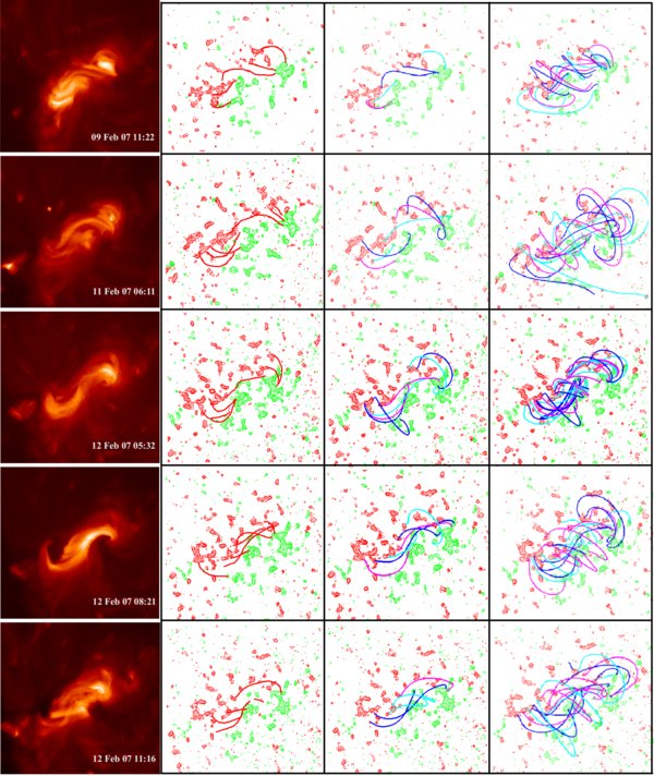
Figure 5. XRT Ti/poly images for the different dates (left column), selected coronal loops from these images (second column), best-fit field lines to the selected coronal loops (third column), and general view of the field configuration (right). Red is the positive polarity, and green is the negative polarity.
Download figure:
Standard image High-resolution imageTable 2. Summary of Best-fit Models
| Date | Φaxi (1020 Mx) | Fpol (1010 Mx cm−1) | AD (R☉) | # loops | L (Mm) | Φ (rad) |
|---|---|---|---|---|---|---|
| Feb 6, 06:11UT | 3 | 1 | 0.0055 | 3 | 80 | 1.7 |
| Feb 6, 06:11UT | 3 | 10 | 0.0057 | 3 | 80 | 16.7 |
| Feb 7, 12:14UT | 3 | 10 | 0.0062 | 6 | 80 | 16.7 |
| Feb 7, 12:14UT | 3 | 5 | 0.0066 | 6 | 80 | 8.4 |
| Feb 7, 12:14UT | 3 | 0.5 | 0.0066 | 6 | 80 | 0.8 |
| Feb 8, 11:29UT | 5 | 1 | 0.0039 | 5 | 95 | 1.2 |
| Feb 9, 11:22UT | 3 | 1 | 0.0041 | 5 | 95 | 2.0 |
| Feb 9, 11:22UT | 5 | 1 | 0.0043 | 5 | 95 | 1.2 |
| Feb 10, 17:59UT | 5 | 1 | 0.0091 | 6 | 119 | 1.5 |
| Feb 11, 06:27UT | 3 | 1 | 0.0067 | 6 | 119 | 2.5 |
| Feb 11, 06:27UT | 3 | 5 | 0.0069 | 6 | 119 | 12.5 |
| Feb 12, 05:32UT | 5 | 3 | 0.0057 | 7 | 99 | 3.7 |
| Feb 12, 05:32UT | 3 | 5 | 0.0060 | 7 | 99 | 10.4 |
| Feb 12, 06:41UT | 5 | 3 | 0.0079 | 6 | 142 | 5.4 |
| Feb 12, 08:38UT | 3 | 0.5 | 0.0050 | 6 | 144 | 1.5 |
| Feb 12, 08:38UT | 3 | 10 | 0.0057 | 6 | 144 | 30.1 |
| Feb 12, 09:26UT | 5 | 0.5 | 0.0042 | 4 | 123 | 0.8 |
| Feb 12, 09:26UT | 5 | 5 | 0.0046 | 4 | 123 | 8.0 |
| Feb 12, 11:15UT | 5 | 0.5 | 0.0057 | 5 | 133 | 0.8 |
| Feb 12, 11:15UT | 5 | 5 | 0.0066 | 5 | 133 | 8.0 |
Download table as: ASCIITypeset image
3.3. Magnetic Structure of the Sigmoid
The models shown in Figure 5 were constructed by inserting a single S-shaped flux rope into the three-dimensional model as described in Section 3.1. The resulting magnetic structure can be described as follows: (1) the magnetic field in the core of the sigmoid is highly sheared in the direction along the PIL. (2) There exist S-shaped field lines in these models that extend along the full length of the sigmoid. (3) The core field is only weakly twisted and exhibits less than one full turn as we follow the field lines from one end of the sigmoid to the other. (4) Surrounding the core is an arcade of field lines that are much less sheared and closer to the potential field. The configuration is similar to that found in previous models (e.g., Titov & Démoulin 1999; Fan & Gibson 2004).
Figure 6 shows magnetic field lines in the model for February 12, 5:32 UT. Here we have selected a series of field lines that range from the interior of the flux rope to the overlying arcade. The left panel shows the field lines in a vertical cross section through the flux rope, and in the central panel the same field lines are plotted on top of the magnetogram as seen from Earth. From these panels it is apparent that field lines that lie close to the core of the flux rope run parallel to the flux rope axis, and with increasing height they become more and more perpendicular, and finally transition to the overlying arcade. This is supported by the right panel of the figure where the model is rotated to the limb and one can see that high-altitude field lines are perpendicular to the flux-rope axis. Such differential shear was previously observed by Schmieder et al. (1996), and is exactly what is expected from the magnetic configuration of a flux rope inserted in a potential arcade. Note that the sheared core field extends only a few hundredths of R☉ above the solar surface; therefore, it is difficult to detect the flux rope in coronagraph observations.
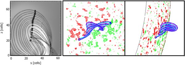
Figure 6. Different views of the flux rope on February 12, 05:32 UT. The left panel shows some field lines projected onto a vertical cross section of the flux rope; the black circles indicate where these field lines cross the vertical plane. The gray scale image shows the distribution of α with lighter gray meaning a higher positive value of α. The center panel shows the same field lines in a view from Earth, plotted on top of the magnetogram. Note how the shear angle of the field lines changes with the height from parallel to the PIL at low heights to perpendicular at large height. On the right, the scene is rotated to the west limb in order to demonstrate the extent of the field lines in height. Red is the positive polarity.
Download figure:
Standard image High-resolution imageAs mentioned above, the single flux-rope models contain S-shaped field lines that extend the full length of the sigmoid. However, on February 12, the overall shape of the sigmoid is reproduced in our model solely by J-like field lines. As discussed in Section 2, this is consistent with the XRT observations and also with what McKenzie & Canfield (2008) report. On the other days, we can see S-shaped coronal loops in the images which match the S-shape field lines from the models. In addition, in the elbows there are J-like field lines that add to the X-ray emission. Therefore, our conclusion differs from the idea presented in McKenzie & Canfield (2008) that the sigmoid is always composed of two J-like structures and is not a single S-shape. From our models we conclude that in cases where the sigmoid seems to be composed of two J-like structures only, the S-shape field lines are more sheared and lie a bit lower than the more potential J-like ones. In Figure 7, one can see one sheared S-shaped field line and two J-like field lines (left) and a vertical cross section along the axis of the sigmoid that gives an impression of the relative height of the three field lines. The overlapping of the J-like field lines with the ends of the S-shaped ones builds up the X-ray emission and the sigmoid acquires a more distinct 2-J shape.
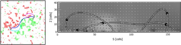
Figure 7. Three model field lines—one S-shaped and two J-like face-on view (left) from 08:21 UT, 2007 February 12, and the same field lines in a cross section along the axis of the sigmoid (right).
Download figure:
Standard image High-resolution imagePevtsov et al. (1996) and Moore et al. (2001) discuss brightenings developing in the center of the sigmoid around the time of eruption. The authors explain these brightenings as resulting from tether-cutting reconnection between two J-like structures. To determine whether a 2-J configuration gives a better fit to the XRT observations prior to eruption, we constructed additional models for February 11 by inserting two flux ropes into the model instead of a single one. This modeling was also inspired by TRACE images that showed the presence of two dark filaments instead of just one at that time. The flux ropes almost touch each other in the center of the sigmoid. We constructed a series of models with different values of the axial and poloidal fluxes, and compared the models to the observations as described in Section 3.2. The average distances were found to be similar to those for the single flux-rope models, and S-shaped field lines still can be seen in the model as a consequence of the interaction of the two flux ropes. We conclude that the 2-J model does not provide a significantly better fit to the observations and thus, we decided to use the single flux-rope model for simplicity.
We could identify the BPSS in our best-fit model fields. Bald patches are parts of filed lines that have low-lying dips and graze the photosphere. The top panel of Figure 8 shows BPs (light and dark blue features) and associated field lines for February 12, 05:32 UT (other dips at larger height are not shown). The bottom panel shows a vertical cross section along the bundle of field lines. One can notice that some of the field lines have a well-defined dip and/or a plateau that reaches well under the flux-rope base. All the field lines shown in this figure define a warped surface that can be identified with a BPSS—for comparison, see w 7 of Titov & Démoulin (1999). The coronal loops that make up the sigmoid lie close to this surface. Based on this figure we can infer that most of the X-ray emission of our sigmoid originates from the region near the BPSS, consistent with the Titov and Demoulin model. Cool filament plasma may accumulate in the dips of the field lines. The position of the dips near the PIL is consistent with the location of filaments along the PIL.
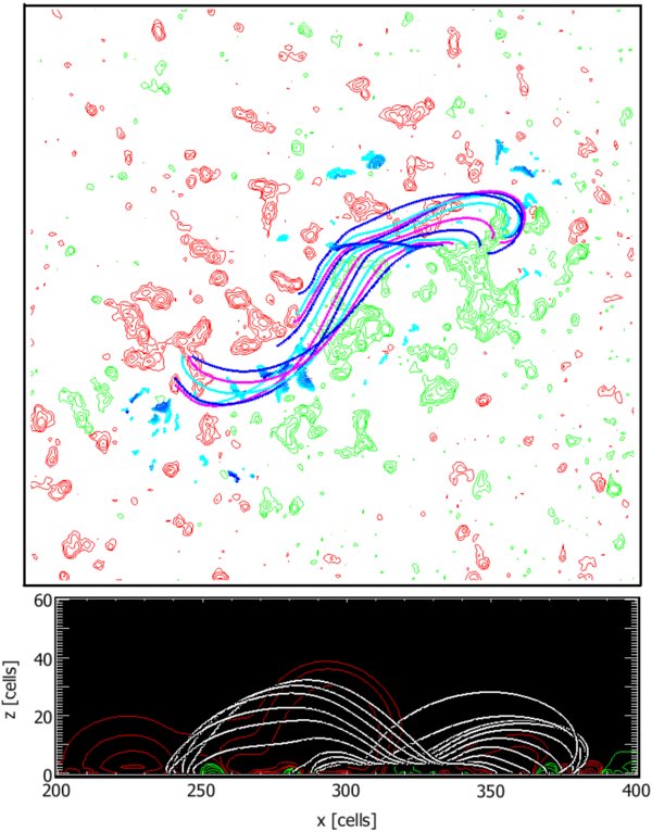
Figure 8. Field lines in the best-fit model for February 12, 05:32 UT. In the top panel, the light and dark blue features show the locations of BPs, which are low-lying dips in the field lines (here drawn at a height of 2–5 Mm). The field lines are traced from these dips. The field lines outline the BPSS that separates the flux rope from the surrounding arcade. The different colors of the field lines help to easily distinguish them. The bottom panel shows a side view of the field lines in a vertical cross section along the length of the sigmoid, demonstrating the dips and plateaus of the field lines. The white field lines correspond to the color ones from the top panel. The green and red contours represent the positive and negative magnetic fields.
Download figure:
Standard image High-resolution image3.4. Evolution Over 7 Days
Figure 5 shows the evolution of the observed sigmoid and the modeled magnetic field from February 9, 11:22 UT to February 12, 11:16 UT. On February 9 (first row in Figure 5) the flux rope is shorter as compared with later days, and the sigmoidal shape is not entirely developed. On February 11 (second row) the sigmoid has reached its final length of about 182 Mm. On February 12 at 5:32 UT (third row) the sigmoid is fully formed, and the axial flux Φaxi of the flux rope is estimated to be (5 ± 2) × 1020 Mx. The fourth row of Figure 5 represents the sigmoid around the time of the eruption that started at about 6:00 UT on February 12. The XRT image from 8:21 UT shows an arcade of short bright loops that cross the PIL in the middle of the sigmoid, similar to post-flare loops. The corresponding magnetic model (shown in column 4) indicates that the axial flux is about (3 ± 2) × 1020 Mx. This is lower than the value for 5:32 UT, but given the large uncertainties in the axial fluxes it is not clear that the difference is real. The last row in Figure 5 shows the post-eruption corona at 11:16 UT when the X-ray sigmoid has largely disappeared. Our modeling indicates that a flux rope is still present at this time.
In Figure 9, we have summarized the results of the best-fit models for all times. The axial and poloidal fluxes of the flux rope, as well as the potential, free, and total magnetic energies and the relative magnetic helicity, are plotted as functions of time. The error bars have been estimated based on the average distances of the best-fit field lines that we determined for each model. Sometimes we find that more than one model can fit the data very well; in this case, the error bars encompass the parameters of all good models. The data points without bars have only one model that is significantly better than the rest, so it is difficult to estimate the errors for such models.
Figure 9. Summary of the model parameters for each observation: axial flux (upper left), poloidal flux (upper right), total energy (middle left), potential energy (middle right), free energy (bottom left), and relative magnetic helicity (bottom right). The start time is 2007 February 6, 06:11 UT.
Download figure:
Standard image High-resolution imageThe potential energy plot shows that the potential energy is smaller on February 6 and 7 while the two regions are separate and the sigmoid is not fully formed. Then it reaches a maximum value and then decreases toward the moment of the eruption. The total energy plot shows the same decrease in time as the potential energy with the lowest value just before the flare brightenings begin (February 12, 06:41 UT). The data points on the free energy plot have large error bars and the behavior of the curve is very erratic which makes it difficult to reach a conclusion based on this curve. Within the error bars the free energy might just as well be constant. On the other hand, the relative helicity plot shows relatively consistent behavior of the curve. The relative helicity seems to build up toward the eruption and then it is suddenly released just before the flare. Then there is indication that the helicity increases shortly after the eruption, but then our data stop and we cannot say if this is an intrinsic and prolonged effect. In general, one might want to put less weight on the data points from February 6 and 7 when the region is still far from the disk center, and the method for estimating the radial field Br from the MDI magnetogram is questionable.
Based on Figure 9 we can infer that the sigmoid stays remarkably stable throughout the length of the observation which comprises the formation and evolution. At the end, the system is disrupted with the appearance of the flare, but there are no clearly identifiable changes in the flux-rope parameters associated with the flare.
4. DISCUSSION
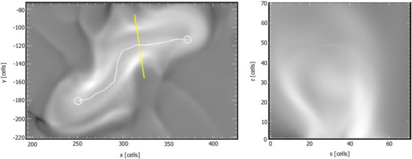
In order to obtain more insight into the structure of the field, we look at the distribution of α(r) in the vicinity of the sigmoid. In Figure 10 (left panel) we have shown this distribution in a horizontal surface at a height of 21 Mm above the photosphere for February 12, 05:32 UT. The brighter regions correspond to areas with higher values of α. Note that there are two ribbons of higher α on either side of the path (white curve) where the flux rope was originally inserted. The right panel of this figure shows the α distribution in a vertical cross section of the flux rope at the location of the yellow line in the left panel. The highest values of α occur at the interface between the flux rope and the envelope field, i.e., the field-aligned currents have a "hollow-core" distribution (Bobra et al. 2008; Su et al. 2009). The reason for this hollow-core distribution is that the magnetic field changes rapidly with the position across the interface, whereas in the central parts of the flux rope the field changes gradually because the flux rope is only weakly twisted. Such current sheets at the boundary of the flux rope were also found in earlier models (Titov & Démoulin 1999; Kliem et al. 2004).
Figure 10. Distribution of the torsion parameter α in a horizontal cross section through the flux rope at a height of 21 Mm (left), and in vertical cross section (right) at the location of the yellow line in the left panel. Bright is the higher value of α; the maximum value is 95 R−1☉. The white curve is the flux-rope path used in the construction of the model. The hollow-core distribution of the electric currents can be seen on both plots.
Download figure:
Standard image High-resolution image
We now consider the stability of our solutions with respect to the ideal-MHD kink mode. Since the solutions were obtained by magneto-frictional relaxation, one expects them to be stable to the kink mode; otherwise the instability would already have developed during the relaxation process. Therefore, we may compare our results with criteria for the kink instability published in the literature. The most relevant works are those in which the arcade surrounding the flux rope is taken into account. Hood & Priest (1980) considered several arcade-like configurations and found that photospheric line-tying has a dominant stabilizing effect. One of these configurations consists of a large flux tube, anchored at its ends and surrounded by an arcade, so that the field transverse to the PIL contains a magnetic island. Such a configuration is found to become unstable if either the length of the structure, the twist of the flux tube, or the height of the magnetic island becomes too great. Instability requires that the twist angle Φ of the flux rope is greater than some critical value, but for Φ < 2π the configuration is definitely stable (see Appendix B in Hood & Priest 1980).
For the present models, the twist angle can be estimated as Φ = 2πFpolL/Φaxi, where Φaxi is the axial flux of the flux rope (in Mx), Fpol is the poloidal flux per unit length along the rope (in Mx cm−1), and L is its length. These parameters are listed in Table 2 for the different models. The boldface model parameters refer to the best fit models in terms of average distance. In addition, in an attempt to estimate the error on these values we also present the closest in AD models with the corresponding twist. Except for February 7, the twist angles Φ (last column of Table 2) are less than 2π rad, which is due to the low value of α in the center of the flux rope as compared to the edge (see Figure 10). There appears to be an increase in Φ from February 11, 06:27 UT until February 12, 06:41 UT (just before the eruption), when Φ ∼ 2π. However, the fact that Φ is less than any of the discussed limits (see the introduction) for the kink instability suggests that the magnetic configuration is stable against the kink mode.
The eruption of the sigmoid occurs between 7:20 UT and 8:20 UT on February 12. While our model does not include the eruption, the XRT observations on the other hand support the standard model of ejective flares (Moore & LaBonte 1980; Moore et al. 2001). According to this model, the two arms of the sigmoid come together in the middle and reach underneath the core field, creating a small region with strong electric currents where reconnection can occur. Magnetized plasma flows horizontally toward the reconnection site, and is ejected in the vertical direction. During an eruption this reconnection becomes a runaway process, creating a vertical current sheet that spreads both in height and in position along the sigmoid. Below the current sheet lies an arcade of "post-flare" loops, and above it lies an elongated structure that lifts off along the entire length of the sigmoid. The reconnection causes the axial field of the sigmoid to split into two parts: an upper part that is ejected and a lower part that remains behind in the low corona (see also Su et al. 2006). In the early stages of the eruption, the post-flare loops are highly sheared because they are formed in an environment where there is a significant component of the magnetic field along the PIL. Later on, the reconnection begins to draw in the envelope field, which is less strongly sheared, so the post-flare loops are less sheared as well. In the present case, the less sheared loops are not seen, perhaps because they are too faint in the late phases of the eruption (February 12, 11:16 UT). Several hours after the eruption there is no sign of the sigmoid, indicating that the coronal field has been significantly reconfigured.
5. CONCLUSIONS
The magnetic configuration of a long-lasting quiescent coronal sigmoid is investigated. NLFFF models of the sigmoid are constructed for several different observations between 2007 February 6 and 12. The modeling uses the flux-rope insertion method (van Ballegooijen 2004; Bobra et al. 2008). A grid of models with different combinations of axial and poloidal fluxes of the flux rope is developed, and each model is checked against the Hinode/XRT observations. We find that the observed features of the sigmoid can be reasonably well fit. We infer that the magnetic field of a sigmoid is highly sheared along the PIL. The configuration can be described as a weakly twisted flux rope surrounded by a potential-field arcade. The axial flux of the flux rope is close to the stability limit, which is about 5 × 10²⁰ Mx for this active region. The field-aligned currents (as indicated by α) are concentrated near the boundary between the flux rope and its surroundings. This current layer more or less coincides with the BPSS (Titov & Démoulin 1999). Most of the X-ray emission appears to come from this current layer.
We also study how the axial and poloidal fluxes, magnetic free energy, and magnetic helicity vary with time. All of these quantities have large uncertainties, and it is difficult to discern clear trends. However, the relative magnetic helicity seems to build up toward the eruption, and a similar trend is found for the twist angle Φ of the field lines inside the flux rope. Although Φ increases with time, we find that the twist angle is less than any of the limits for the kink instability. This is consistent with the observed long-term stability of the magnetic structure. We conclude that the eruption is most likely not due to the kink instability, and another kind of eruption mechanism must be explored in order to explain the X-ray flare.
Hinode is a Japanese mission developed, launched, and operated by ISAS/JAXA in partnership with NAOJ, NASA, and STFC (UK). Additional operational support is provided by ESA, NSC (Norway). This work was supported by NASA contract NNM07AB07C to SAO. We also thank the referee for very useful comments which helped making this work better.
Footnotes
- 1
- 2