


ABSTRACT
This paper shows results from experiments diagnosing the development of the Rayleigh–Taylor instability with two-dimensional initial conditions at an embedded, decelerating interface. Experiments are performed at the Omega Laser and use ∼5 kJ of energy to create a planar blast wave in a dense, plastic layer that is followed by a lower density foam layer. The single-mode interface has a wavelength of 50 μm and amplitude of 2.5 μm. Some targets are supplemented with additional modes. The interface is shocked then decelerated by the foam layer. This initially produces the Richtmyer–Meshkov instability followed and then dominated by Rayleigh–Taylor growth that quickly evolves into the nonlinear regime. The experimental conditions are scaled to be hydrodynamically similar to SN1987A in order to study the instabilities that are believed to occur at the He/H interface during the blast-wave-driven explosion phase of the star. Simulations of the experiment were performed using the FLASH hydrodynamics code.
Export citation and abstract BibTeX RIS
1. INTRODUCTION
Blast-wave-driven instabilities are important phenomenon that have consequences in several areas including, but not limited to, astrophysics (Ribeyre et al. 2004) and Inertial Confinement Fusion (ICF; Lindl 1998). Blast waves occur following a sudden, finite release of energy, and consist of a shock front followed by a rarefaction wave. Many explosions, including stellar explosions, lead to the development of blast waves. Other examples of blast wave occurrences include the collision of a comet with a planet or planetary atmosphere (McGregor et al. 1996) and the interaction of the solar wind with the energy released from a solar flare (Drake 2006). A blast wave creates a pressure gradient in the direction of its propagation. If the structure of a system produces a density gradient in an opposing direction to the pressure gradient then the Rayleigh–Taylor (Rayleigh 1900; Taylor 1950) instability will occur. This will happen when a blast wave crosses an interface or transition where the density decreases.
The Rayleigh–Taylor instability is also a common process, occurring whenever denser fluid is accelerated against less dense fluid, whether in a gravitational field or otherwise. The Rayleigh–Taylor instability occurs in core-collapse supernova (SN) explosions when the blast wave moves outward across transitions of more-rapidly decreasing density (Arnett et al. 1989; Bandiera 1984; Chevalier 1976; Falk & Arnett 1973; Fryxell et al. 1991; Hachisu et al. 1990; Herant & Benz 1991; Herant et al. 1992; Muller et al. 1991; Shigeyama & Nomoto 1990; Shigeyama et al. 1988) and in young supernova remnants as the stellar ejecta are decelerated by the shocked circumstellar medium (Chevalier et al. 1992). Rayleigh–Taylor is also evident in the Crab Nebula, at the boundary of the pulsar-wind nebula, where hot gas from the SN explosion is accelerated into the surrounding interstellar medium creating a fingerlike structure (Hester et al. 1996). Imperfections in the target or nonuniform laser irradiation induce the Rayleigh–Taylor instability in ICF experiments. The performance of an ICF target is limited by the growth of hydrodynamic instabilities. Also, because of the mixing brought on by the Rayleigh–Taylor instability, the further understanding of this phenomenon may lead to a better understanding of turbulent mixing (Zhou et al. 2003).
The experiments described in the present paper focus on the Rayleigh–Taylor instability at the blast-wave-driven He/H interface in a core-collapse SN, with a specific focus on SN1987A. This SN has been widely studied, due in part to its close proximity to Earth, at about 50 kpc. It is also of great interest because some heavy elements were observed earlier than anticipated and had larger than expected Doppler shifts. The mechanism for the transport of heavy, core elements through the star at very high velocities has led to a number of computer simulations of the exploding star (Shigeyama et al. 1988; Shigeyama & Nomoto 1990; Arnett et al. 1989; Fryxell et al. 1991; Hachisu et al. 1990; Herant & Benz 1991; Herant et al. 1992; Muller et al. 1991; Kifonidis et al. 2000; Kifonidis et al. 2003; Kifonidis et al. 2006). At present, only one simulation has been able to produce metal-rich material moving at velocities approaching the observed values, using a specific model of anisotropic neutrino-driven convection (Kifonidis et al. 2006). However, a fully three-dimensional calculation of the entire star with realistic perturbations on all relevant interfaces is not currently feasible, and in addition current simulations are limited to a numerical Reynolds number, Re, below the turbulent transition threshold at ∼20,000 (Dimotakis 2000). Therefore, it is worthwhile to further study material transport mechanisms that may be present in this or similar SNe by means of relevant, well-scaled (Ryutov et al. 1999) experiments having Re above the transition threshold.
The system of interest can be scaled to an experiment performed with a high-powered laser (Ryutov et al. 1999). This is possible only because these two systems, the experiment and the relevant part of the SN, satisfy similarity conditions based on the Euler equations so their hydrodynamics will evolve in a similar way. Both systems remain invariant under a transformation of the Euler equations. The Euler equations can be used to describe both SN1987A and a well-scaled laboratory experiment if several conditions are met. First, both systems must be highly collisional. In both the experiment and the SN, the collisional mean free path is much smaller than the characteristic scale height of the system, so both systems are indeed highly collisional. Second, heat conduction must be negligible. Both systems have high Peclet numbers, which is the ratio of heat convection to heat conduction, so we can neglect heat conduction for both systems. For the SN, Pe ∼ 1012 and for the laboratory experiment Pe ∼ 103. Also, the radiation flux must be small. For the SN, the photon Peclet number, Peγ, which is inversely proportional to the thermal diffusivity for photons, must be considered. Since Peγ is ∼1016 for the SN we can neglect radiation flux for that system. However, Peγ is difficult to estimate in the experiment. Therefore, the blackbody cooling time must be used to estimate the effects of radiation flux. For the experiment, the blackbody cooling time is much longer than the characteristic hydrodynamic time. Also, viscosity must be negligible. In both systems the Reynolds number, which is the ratio of the inertial force to viscous force, is large. For the experiment, the Reynolds number is ∼105 and for the SN, Re ∼ 2 × 10¹⁰. While the Re, Pe, and Peγ numbers for the two systems are different they are both sufficiently large so that the corresponding effect is minimal. Furthermore, gravitational and magnetic forces must be negligible. In an SN explosion, the acceleration due to the explosion is far greater than acceleration due to gravity. Also, the magnetic pressure is small compared to the plasma pressure during the explosion phase. With all of these conditions met, we can conclude that for a finite amount of time the hydrodynamic evolution of these two systems will be similar.
When designing our experiment it is also important that the boundary conditions in space and time are also scaled to those in the SN. Figure 1(a) shows one-dimensional simulations performed with the Prometheus code (Fryxell et al. 1991) code of the He/H interface velocity in SN1987A versus time as well as the experimental interface velocity versus time, which was simulated using the Hyades code (Larsen & Lane 1994) code. These images were adapted from Kane et al. (1999) and Drake et al. (2002). This plot has different time and velocity scales for the experiment and the model SN, but the motion of the interface has the same shape in both cases. This is also true for the profiles of pressure and density near the interface as seen in Figures 1(b) and (c). One can see that the structures of pressure and density are very similar between the experiment and the model star, although they are not strictly identical. These similarities in spatial and temporal structures imply that the evolution of the two systems will be similar, and certainly should exhibit the same instability mechanisms for some period of time.
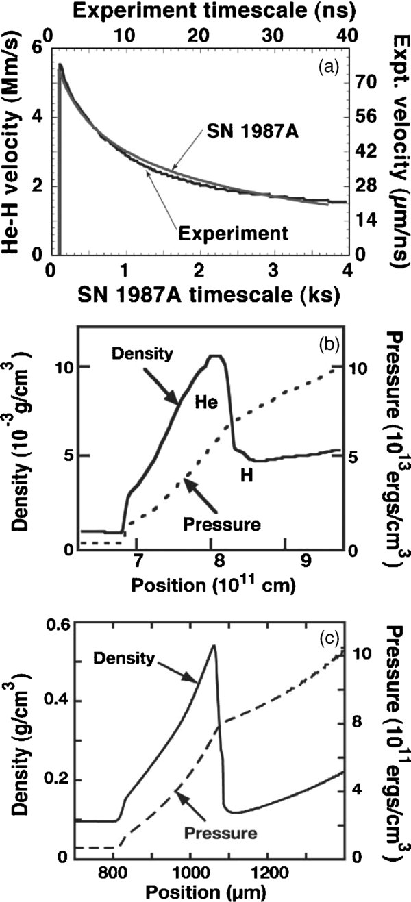
Figure 1. Comparison of (a) interfacial velocity, pressure, and density in the (b) star and (c) laboratory experiment. Although the two systems are shown on different scales they have similar profiles. These plots were adapted from Kane et al. (1997) and Drake et al. (2002).
Download figure:
Standard image High-resolution imageHowever, it should be noted that there are some limitations in the correspondence between the experiment and the SN. The two materials in our experiment are an approximation of the density change in the outer layers of the SN. In contrast to the experiment, which initially has layers of uniform density, the density of an individual layer in a star is not uniform within a layer. However, there is a much more rapid density change at the interface between two layers in the SN. Once the blast wave crosses the interface the shape of the density profile for the experiment and SN1987A are similar as discussed above. Also, the target itself is only representative of a small portion of the SN since it is planar and not spherical. This leads to the experiment only being well scaled for a finite amount of time. Once the disturbances from the edges of the target reach the center of the target the experiment is no longer scaled to the SN. Even with these limitations, during the length of the experiment, up to 30 ns, the hydrodynamic instabilities that occur in the experiment are similar to those that are thought to be responsible for the observed characteristics of core-collapse SN (e.g., SN1987A).
2. EXPERIMENTAL CONDITIONS
These experiments were conducted using millimeter-scale targets designed to create a similar, scaled interfacial acceleration history to the blast-wave-driven H/He interface during the explosion phase in SN1987A. This target can be seen in Figure 2. The target body consists of a Be washer and shock tube. The washer has an inner and outer diameter of 950 μm and 2.5 mm, respectively. This washer is used to protect the diagnostics and outer target from the laser beams. In some cases, a gold washer coated with a thin layer of plastic was used instead of the Be washer. The Be shock tube holds the target package and has a 1.1 mm outer diameter and 150 μm thick, Be walls. Inside the tube is a disk, 800 μm in diameter and 150 μm thick of polyimide (a type of plastic), which has a chemical composition of C22H10O5N2 and a density of 1.41 g cm−3. Behind the plastic disk is 2–4 mm of carbonized resorcinol formaldehyde (CRF) foam with a density of 100 mg cm−3. After the passage of the blast wave, the density jump between the plastic disk and the foam provides a density jump similar to that of the hydrogen and helium interface in SN1987A as was discussed in the previous section and shown in Figure 1. A gold grid is placed on the outside of the shock tube for calibration of position and magnification of the resulting radiographic images. Figure 2(a) shows a cross section of the target described above and Figure 2(b) is an image of the target. This target had a plastic-coated gold washer and is mounted on a glass stalk. The two fibers protruding from the target are used for alignment of the target in the Omega chamber. The large foil attached to the target is a Ti backlighter and will be further discussed later in this paper. These targets were fabricated at Lawrence Livermore National Laboratory.

Figure 2. Experimental target (a) shown in a cross section with a washer and shock tube. Inside the shock tube is a high-density plastic layer and a lower density foam layer. The plastic layer has a seed perturbation machined at the interface between the two materials. The laser beams irradiate the plastic component of the target. Part (b) shows a photograph of the target. This target has an Au washer. This image also shows the glass stalk on which the target is mounted and gold fiducial grid. The backlighter foil is positioned 4 mm from the target opposite the diagnostic, a gated X-ray framing camera.
Download figure:
Standard image High-resolution imageOn the rear surface of the polyimide disk a 75 μm thick, 200 μm wide slot was milled out of the plastic. A "tracer" strip of C500H457Br43 (CHBr) with a density of 1.42 g cm−3 was glued into this slot. The tracer strip was used because the bromine component in the CHBr more readily absorbs the 4.7 keV backlighter X-rays than the surrounding plastic material. X-ray radiography was the primary diagnostic of this experiment so the bromine provides contrast in the radiographic images. CHBr and polyimide are predominately low Z and have similar densities, therefore, the two materials will have a similar hydrodynamic response to the extreme pressure created by the laser beams incident upon the target. Also, since the tracer strip is in the center of the target it allows the diagnostic to "look through" the polyimide surrounding the strip and Be shock tube since they are both nearly transparent to the X-rays used to diagnose the experiment. This allows the radiograph to diagnose primarily a slice through the center of the target, unaffected by edge effects along any given line of sight. Also, one experiment was performed without a shock tube to learn how the interaction with the tube walls affects the results.
Several different types of two-dimensional sinusoidal patterns have been machined onto the rear surface of the plastic disk. These patterns serve as a seed perturbation for the Rayleigh–Taylor instability. The purpose of these patterns is to determine whether or not more complex seed perturbations lead to the displacement of more material. The basic machined pattern is a single-mode sine wave, a0cos(k1x) where a0 = 2.5 μm and k1 = 2π/(50 μm). The majority of experiments performed with a single-mode perturbation were done with the aforementioned specifications; however, some of the experiments had target interfaces with a longer wavelength single-mode pattern, where a0 = 2.5 μm and k1 = 2π/(100 μm). For clarity, the former perturbation will be referred to as single mode and the latter will be referred to as long-wavelength single mode. The more complex patterns have additional sine waves added to the basic pattern. The two-mode pattern is defined by
Also, there is an eight-mode perturbation defined by
where λi = (180 μm)/i. The amplitude components, ai, range from 0.4 μm to 0.7 μm and are shown in Table 1, with the total amplitude for the multimode perturbation being ∼2.5 μm, similar to the two-mode and single-mode patterns. Cross sections of these three perturbations can be seen in Figure 3. The experimental perturbations were chosen based on the length scale of the system as well as the ability to easily diagnose the growing perturbation.

Figure 3. Cross sections of the (a) single-mode (one-mode), (b) two-mode, and (c) eight-mode seed perturbations. The patterns are machined onto the plastic component of the target in one direction as a ripple. The overall amplitudes of all the patterns are similar.
Download figure:
Standard image High-resolution imageTable 1. Description of the Eight-Mode Perturbation
| i | λi | ai |
|---|---|---|
| 1 | 180 | 0.602669 |
| 2 | 90 | 0.502309 |
| 3 | 60 | 0.526604 |
| 4 | 45 | −0.683793 |
| 5 | 36 | 0.564115 |
| 6 | 30 | −0.625269 |
| 7 | 25.7143 | −0.474363 |
| 8 | 22.5 | −0.546737 |
Notes. The subscript, i, indicates a specific mode, λi and ai, indicate the wavelength and amplitude of that mode, respectively. Note that λi = 180 μm/i and the total amplitude of the pattern is ∼2.5 μm.
Download table as: ASCIITypeset image
Some of the plastic components were machined with a flat surface. Experiments using such targets can determine the position of the one-dimensional, or "mean," fluid interface. In contrast, due to extensive material mixing, one cannot directly determine the actual mean interface position in experiments with sinusoidal surfaces, as one cannot determine the relative amplitude of the spikes and the bubbles. The best one can then do is to estimate the mean interface position from the midpoint between the bubbles and spikes. All of the plastic components, the planar and patterned surfaces, have some amount of small grooves due to the tools used in the machining process. This surface roughness is akin to having additional short-wavelength, small-amplitude modes on the surface. These modes, while small, will still cause some Rayleigh–Taylor growth, however, on the sinusoidal patterns these small modes will be damped and the larger modes will dominate.
Ten Omega (Boehly et al. 1995) laser beams with 1 ns flat-topped pulse shapes irradiate the dense plastic disk of the target. The laser beams have a wavelength of 0.35 μm. Each beam passes through a distributed phase plate (DPP) that produces a spot size of 820 μm FWHM that is smooth overall with fine speckles on a 5 μm scale. The total energy of the beams is ∼5 kJ and the average irradiance is ∼9.5 × 10¹⁴ W cm−2, producing an ablation pressure of ∼50 Mbar in the plastic layer of the target. This large pressure difference in the plastic layer creates a strong shock wave.
This shock wave traverses about halfway through the 150 μm dense plastic layer in the 1 ns while the laser is activated. After the laser pulse ends, the plasma that has been created is allowed to freely expand away from the irradiated surface. This causes a rarefaction wave, a decrease in density and pressure due to outward flow, to overtake the shock wave. Then the initial, abrupt acceleration of the shock is followed by the extended deceleration in the rarefaction, creating the desired planar blast wave structure moving toward the interface between the plastic and foam. At ∼2.2 ns the blast wave crosses this interface, launching a forward shock into the foam. The density ratio between the plastic and the foam is greater than can be sustained by a single shock, which is accompanied by a backward moving rarefaction. This rarefaction causes the plasma behind the interface to accelerate and begin to accumulate at the interface. The accumulation of shocked foam ahead of the interface causes it to decelerate relative to the plasma flowing toward the interface from the denser matter. As the ram pressure of the inflowing plasma, in the plane of the interface, increases above the thermal pressure of the shocked foam a reverse shock forms.
The creation of this blast wave structure was simulated using the Hyades code, a one-dimensional, Lagrangian, code with a multigroup flux-limited diffusion radiative transport model. Although the radiation transport model is not as accurate as the full treatment of the radiative transfer equation and while two-dimensional effects play an important role in our experiments, one-dimensional Hyades remains a useful tool for experimental scoping and analysis. In its Lagrangian description, the computational mesh that describes the target moves with the material so that each element of mass in the mesh is conserved over time. Hyades uses equations that describe a three-temperature, single fluid. The pressure in the continuity and momentum equations represent the summed contributions from electrons, ions, and radiation. There is an energy equation for ions, for electrons, and for each radiation group. Electron heat transport is approximated by flux-limited diffusion. The multigroup radiation method allows the user to assign energy ranges to many different photon groups, for each of which the opacity is calculated using an average atom model.
Simulation codes similar to Hyades are known to overestimate the ablation pressure when run in one-dimension with an actual laser irradiance in the range of the present experiments (Reighard et al. 2007). This is due at least in part to the absence of lateral heat transport in one dimension. In order to correct for this unrealistically large ablation pressure the laser irradiance is reduced in simulations. To quantify this reduction, Hyades runs were performed at different irradiances and the shock and mean interface positions were found. The mean interface is defined at the average of the Rayleigh–Taylor spike-tip and bubble-tip positions. These positions were compared to the experimental shock and mean interface positions. These results are shown in Figure 4. It shows that Hyades, run with a laser irradiance of 6.0 × 10¹⁴ W cm−2, or about 60% of the actual value, best represents the experimental data. The positions of the shock and mean interface are also shown for 50% and 70% of the nominal laser irradiance. One can see that variations of about ±10% in the reduced laser irradiance do not reproduce the data nearly as well.
Figure 4. Plots of shock and interface positions vs. time for the experiment and Hyades simulation at several different laser intensities. The laser intensities are 50%, 60%, and 70% of the nominal laser energy. The shock and interface positions are shown as lines, with the shock positions being greater than the interfaces positions. The experimental shock position is shown with open circles and the experimental mean interface position, the average of the spike-tip and bubble-tip position, is indicated with black circles. The gray triangle indicates the position of the interface in a target machined with a flat interface i.e., no perturbation.
Download figure:
Standard image High-resolution imageEven though using an irradiance of 6.0 × 10¹⁴ W cm−2 matches the general trend in the data, one can see that there is a large dispersion of experimental data points. For example, at t = 13.4 ns the shock position varies by ∼150 μm and the interface position by ∼100 μm. These differences are comparable to the lengths of the spikes and bubbles in the experiment. These shot-to-shot variations are most likely due to small differences (e.g., laser energy, target alignment, target fabrication, target metrology) in the experiment, which lead to errors in the inferred absolute position of features. Of these variations, the laser energy for each shot is well known. For the data shown in this paper the laser energy generally varied by about ±7%. However, for three of the shots, the laser energy varied by 30% due to a reduction of beams. These variations cause a change in the shock and interface position of ∼6%.
A simulation of how the desired blast-wave structure is created can be seen in Figure 5. Figure 5(a) is a plot of density versus position, Figure 5(b) is a plot of pressure versus position, and Figure 5(c) is a plot of velocity versus position. Each line on the plots represents a different time. These plots are at t = 0 ns, 1.0 ns, 2.0 ns, and 4.0 ns. The gray, dashed line in the density plot shows the initial condition (t = 0 ns) of the dense plastic layer followed by the lower density foam. The laser beams irradiate the plastic and in this case would come from the left side of the plot. At t = 1.0 ns the pressure is ∼5 × 10¹³ dynes cm−2 or ∼50 Mbar, which has caused a shock wave, visible at ∼65 μm moving at ∼52 km s−1. At 1 ns the laser beam pulse has ended and by 2.0 ns a blast wave has developed with the leading edge at ∼130 μm from the front surface of the target. The blast wave crosses the interface ∼2.2 ns and the forward shock is then launched into the foam. At 4.0 ns the shock is moving at ∼58 km s−1 and located at ∼270 μm while the interface behind it is moving at ∼54 km s−1 and is located at ∼240 μm.

Figure 5. Plots from Hyades simulations showing density (a), pressure (b), and velocity (c) vs. time. Each line on the plot indicates a different time during the experiment. The times shown are t = 0 ns, 1.0 ns, 2.0 ns, and 4.0 ns. The density plot best illustrates the formation of a blast wave. The initial condition of a dense layer followed by a lower density layer is shown at t = 0 ns. The laser beams irradiate the plastic material and a shock wave forms by 1 ns. The laser pulse ends allowing the material to decompress and a rarefaction forms. This rarefaction wave overtakes the shock wave forming a blast wave. The blast wave crosses the interface at ∼2.2 ns.
Download figure:
Standard image High-resolution imageThe experiment is observed at times much later than when the shock crosses the interface. Figure 6 shows results of Hyades simulations of the experiment at times of 8, 14, 20, and 26 ns. At 8 ns the shock can be seen at ∼575 μm, the interface is at ∼450 μm. At this time, the shock and interface have slowed down considerably to 50 km s−1 and 42 km s−1 and they continue to decelerate. By 26 ns, the shock and interface have moved to have 1500 μm and 1000 μm, respectively.

Figure 6. Hyades simulation of density vs. position for late times: t = 8 ns, t = 14 ns, t = 20 ns, and t = 26 ns.
Download figure:
Standard image High-resolution imageThe acceleration of the interface due to the planar blast wave is similar to the model SN and our experiment as discussed earlier. The interface is unstable to the Richtmyer–Meshkov (Richtmyer 1960; Meshkov 1969) instability due to the strong shock crossing the interface and Rayleigh–Taylor instability due to the deceleration phase behind the shock front. Similar dynamics are believed to occur within a core-collapse SN in which the dense, core layers are shocked then decelerated by the less dense, outer layers. In the experiment, the Richtmeyer–Meshkov instability dominates in the first few nanoseconds, but the rate of amplitude increase quickly becomes small compared to the growth rate of the Rayleigh–Taylor instability (Robey et al. 2003). This experiment is observed when the Rayleigh–Taylor growth is dominant.
The main diagnostic during this experiment is X-ray radiography using a gated X-ray framing camera (Budil et al. 1996). As can be seen in Figure 2, an area backlighter, a 4 × 4 mm, 5 μm thick Ti foil is attached to the target via a 4 mm long wire. The backlighter is placed on the side of the target that is opposite the diagnostic. The material of the foil is chosen by matching the energy of the He-α emission of the foil to ∼10% transmission of radiation through the target estimated using a cold opacity library. In this experiment Ti was used for an He-α energy of 4.75 keV. Six to eight Omega beams with 670–750 μm spot size irradiate the front and back of this foil creating X-ray photons, at some time delayed 8–26 ns from the leading edge of the drive beams. These photons pass through the target and are imaged by a 4 × 4 array of pinholes and a gated X-ray framing camera (Budil et al. 1996).
At the front of the framing camera is a microchannel plate (MCP) that generates electrons from the incoming X-ray photons. The electrons are accelerated and multiplied by a gating pulse. Behind the MCP is a phosphor plate that is at 5 kV while the back of the MCP is at ground. The positive potential accelerates the electrons so that they emit light when they strike the phosphor plate. These visible photons then go to a CCD camera or film.
The result is a set of 16 images on four strips. The time delay between the rows is adjustable and was typically set to 200 ps. The images along a given strip, separated in time by 70 ps, are analyzed to give a single shock and interface position at an appropriately averaged time. When the diagnostic is well aligned and works well, one obtains several measurements of positions on a given shot. This can be seen in Figure 4 where there are several points clustered in one area. The features measured on these images for this paper are the shock position, spike-tip position, and bubble-tip position. Recall that Figure 4 shows the mean interface position, which is the average of the spike-tip and bubble-tip positions. The positions of these features are found by taking a one-dimensional profile across the feature. The pixel intensity in the image will vary across the specific feature. The position is determined to be halfway between the start and end of the variation in intensity. This leads to an error in the measurement of about 10 μm for each feature. In Figure 4, one can see that the positions of the mean interface and shock has a fluctuation of greater than 10 μm or, combining the error of the spike and bubble position, 14 μm in the case of the mean interface. This is due to the shot-to-shot variations discussed previously, which affects the absolute calibration of the radiographic images. This leads to a variation approaching ±10% in the calibrated data.
3. EXPERIMENTAL RESULTS
Radiographs of experiments performed using targets with a single-mode interface can be seen in Figure 7. These images are of the single-mode interface with a 50 μm wavelength. The results of targets having a longer wavelength (100 μm) single-mode pattern are not shown, but are very similar to the images in Figure 7. It is worth noting some features in this and following images. The target coordinate x = 0 μm is at the front surface of the dense plastic material where the laser beams irradiate the target and the target coordinate y = 0 μm is at the axis of the target. Figure 7(c) has a triangular region in the upper right corner of the image where the detector was not active. In these images the shock can be seen, as the rightmost transition. The interface has become convoluted, so that one sees dark features extending to the right and light features extending to the left. The dark fingers are spikes of dense material moving to the right. In between the spikes are bubbles of lower density material moving to the left relative to the interface. The spikes and bubbles at the interface are due to the Rayleigh–Taylor and Richtmeyer–Meshkov instabilities. In Figure 7(a), the shock is visible ahead of the interface at ∼550 μm. The reverse shock, at the left edge of the dark vertical feature, is at 400 μm. Further to the left one can see the left edge of the CHBr.

Figure 7. X-ray radiographic images of experiments performed with targets that had a single-mode pattern machined on the plastic component. In each image, the interface and shock wave are moving to the right. The images were taken at the following times: 8 ns (a), 12 ns (b), and 26 ns (c).
Download figure:
Standard image High-resolution imageFigures 7(a)–(c) are taken at t = 8 ns, t = 12 ns, and t = 26 ns after the drive beams irradiated the target, respectively. In these radiographs, note the increasing distance between interface and the shock as well as the decrease in definition of the interface and the reverse shock at later times. Also, note that the spikes appear longer at later times; this is due to both the unstable growth and the gradual expansion of the system as the pressure decreases. Figure 7(b) clearly shows some roll-up on the edges of the target due to Kelvin–Helmholtz effects from the interaction between the plasma and the tube walls. In all of these images the tips of the spikes appear to be thicker than the rest of the spike structure, which is also due to Kelvin–Helmholtz effects.
Experimental images of targets with a two-mode perturbation can be seen in Figures 8(a)–(c). These radiographs were taken at 13, 20, and 26 ns after the start of the initial laser pulse. Along the top of the image a gold calibration grid can be seen. In Figure 7(a), the modal structure of the perturbation can be clearly seen. This definition of the structure decreases with time until it is no longer readily visible at 26 ns. Radiographs of the eight-mode interface are shown in Figures 9(a) and (b) at 13 and 26 ns, respectively. Again, the modal structure is quite distinct early in time. The structure is less definite at t = 26 ns, but it is still visible. Figure 9(c) shows a radiographic image of a target with a planar interface taken at 8 ns. The interface is visible at ∼500 μm and is moving to the right, but the forward shock and reverse shock cannot be seen in this image.

Figure 8. X-ray radiographic images of experiments performed with targets that had a two-mode pattern machined on the plastic component. The images were taken at the following times: 13 ns (a), 20 ns (b), and 26 ns (c). The complex structure is very different from the single-mode pattern and is due to the initial conditions.
Download figure:
Standard image High-resolution image
Figure 9. X-ray radiographic images of experiments performed with targets that had an eight-mode pattern machined on the plastic component. Theses images were taken at 13 ns (a) and 26 ns (b). Part (c) shows an X-ray radiograph of a target with a planar interface taken at 8 ns. The interface is visible at ∼500 μm and is moving to the right. The forward shock is not visible in this image.
Download figure:
Standard image High-resolution imageThe radiographic images shown in this paper have been calibrated using the gold grid. The spacing between grid wires is 63 μm, which is used to find the magnification of the image. For these images, the nominal magnification is 8, but the actual value varies between 7.84 and 8.97. The magnification varies due to errors in target alignment, location of the area backlighter, and location of the X-ray framing camera. The location of the grid is measured with respect to the driven surface of the target prior to the experiment. Using the grid location and magnification, the absolute positions of the shock, spike-tip, and bubble-tip, and other features are found.
The mean interface in experiments performed with a machined sinusoidal pattern is defined here as the average of the spike-tip and bubble-tip positions. The analysis was performed this way because the unperturbed interface position is not known. An experiment was performed using a plastic component that was machined to a flat surface in order to compare with the mean interface of an experiment executed with a machined perturbation. The gray diamond symbol shown in Figure 4 indicates that the planar interface (t = 8 ns) falls on the curve of the mean interface position versus time, and shows the mean interface from all the experiments with machined patterns. These are certainly consistent within the experimental variability.
The spike-tip and bubble-tip position versus time for different types of perturbations can be seen in Figure 10. This shows how far the spikes have penetrated into the foam material with respect to time, and that the total spike penetration is generally increasing with time. The error bars in this image are roughly the size of the symbol and therefore, are not shown. For the multimode experiments, where some spikes penetrate farther than others, the position of the spike-tip shown is referring to the farthest protruding spike. Likewise, the bubbles are moving in the opposite direction, while the entire interface is moving due to the background fluid motion. This plot also shows the mean interface from a one-dimensional Hyades simulation indicated by the black line. The spike-tip and bubble-tip positions generally fall on either side of the simulated interface, as expected. However, this figure shows a rather large spread in data and in some cases shows a spike-tip (bubble-tip) in front of (behind) the mean interface giving nonsensical negative amplitude for the feature. In order to accommodate the large spread in data while still being able to draw a meaningful conclusion, this paper will refer to the mix-layer amplitude, half the distance between the spike and bubble, as a surrogate for individual spike and bubble amplitudes.

Figure 10. Plot of spike-tip and bubble-tip positions vs. time. Targets with different seed perturbations are differentiated by different triangles. The mean interface from a Hyades simulation is also plotted and indicated by line shown. The error bars for this data are smaller than the symbol size and therefore, not shown.
Download figure:
Standard image High-resolution imageFigure 11 shows the amplitude of the mix layer versus time. The mix-layer amplitude is also increasing with time. These data points generally fall on a straight line and based on these data one cannot resolve a difference due to the type of perturbation used during the experiment. There are three outliers in this plot, which will be discussed. The point labeled A was an experiment performed without a Be tube. One can hypothesize that the system was able to freely expand laterally and that this led to less forward growth of the interface. The point labeled B was a two-mode experiment and the result is seen in Figure 8(b). The analysis of other two-mode experiments found the position of the most protruding spike, however, in Figure 8(b) the only spikes visible are the shorter spikes. This would account for the smaller mixing layer amplitude. Point C is an eight-mode experiment seen in Figure 9(b). Due to the poor contrast in this image it is unlikely that the end of the spike can be seen and therefore it has smaller amplitude. These three outlying points are deleted from later plots.

Figure 11. Plot of mix-layer amplitude for the varying seed perturbations used for these experiments. The mix-layer amplitude is defined at the spike-tip position subtracted form the bubble-tip positions and divided by 2.
Download figure:
Standard image High-resolution image4. TWO-DIMENSIONAL SIMULATIONS
Simulations of these same experiments were previously performed using the simulation code CALE and were reported by Miles et al. (2004) The simulations presented in this paper were performed using the FLASH code (Fryxell et al. 2000) code. FLASH is used to model general compressible flow problems common to complex astrophysical systems. This multidimensional code solves the Euler equations using the Piecewise-Parabolic-Method (PPM; Colella & Woodward 1984). FLASH allows for adaptive mesh refinement, using a block-structured adaptive grid and placing resolution elements only in areas where refinement is needed most. These simulations were performed using two-dimensional Cartesian geometry. A gamma law equation of state (EOS) model was used with gamma defined as 1.4 for both the plastic and foam (appropriate for the partially ionized media used here (Drake 2006)).
The FLASH code does not include the means to accurately model what happens while a laser is irradiating a material. Therefore, the output from a one-dimensional Hyades simulation is used as input for a FLASH simulation to set the initial conditions of the simulation as a laser irradiance. The initial setup is the same as for the Hyades simulations described above except that the perturbations used in the experiment have been included. These simulations did not include the Be tube that is used in the experiment. However, the boundary where the tube would be, parallel to the target's symmetry axis, is set to be reflective. The boundaries perpendicular to the target's symmetry axis are out-flowing.
The simulations were set to refine in areas where there was a large change in pressure and concentration of polyimide between neighboring zones. This allows for refinement near the interface and the shock. The domain of this simulation was the size of the inner diameter of the Be tube in the experiment. The resolution for the single-mode and two-mode simulations was about 0.78 μm, corresponding to >50 resolution elements per wavelength for the smallest wavelength. The simulation for the eight-mode pattern was performed at higher resolution, 0.39 μm but at similar resolution elements per smallest wavelength. Resolution studies on similar systems have shown that this resolution is sufficient and that results with a higher resolution simulation will only differ in the small-scale structure (Calder et al. 2002; Miles et al. 2004).
Figure 12 shows results from FLASH simulations for three different types of initial conditions. These images plot the density of the simulation where the darkest region indicates the densest feature. Figure 12(a) shows a FLASH simulation at t = 12 ns with a single-mode initial perturbation. This can be compared to an experimental radiograph at the same time in Figure 7(b). Simulations were also done with a long-wavelength single-mode pattern, but are not shown, as they are very similar to the simulations shown in Figure 12(a). Figure 12(b) shows a FLASH simulation with a two-mode initial perturbation at t = 13 ns. An experimental radiograph with the same initial condition and time is shown in Figure 8(a). Figure 12(c) shows a simulation of a target with an eight-mode initial perturbation at t = 13 ns. The analogous experimental radiograph is shown in Figure 9(a).
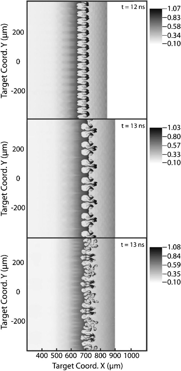
Figure 12. Two-dimensional density plots from FLASH simulations of (a) a one-mode experiment at t = 12 ns, (b) a two-mode experiment at t = 13 ns, and (c) an eight-mode experiment at t = 13 ns.
Download figure:
Standard image High-resolution imageOverall, the mix-layer amplitude resulting from the simulations shows good qualitative agreement with the mix-layer amplitude from the experiments. Due to the higher resolution of the simulation, more detail can be seen than in the radiographs. Also, the shocks in Figure 12 are very flat, while the shocks and interface appeared to be slightly curved in the experimental radiographs. These simulations do not contain a Be tube as the experiment does, therefore, the edges of the simulation domain are not slowed down by interaction with the tube. Also, the edges of the domain do not expand laterally as Be tube does during the experiment. This will cause the shock to appear overly planar in the simulation and move faster than the shock wave in the experiment. Finally, the initial laser condition was set by a one-dimensional Hyades simulation with flat laser irradiance. In the experiment, the laser irradiance profile has a curved shape due to the overlapping of several beams. This causes the ablation pressure to be largest in the center of the target causing the shock and interface velocity to be larger at that point. This will position the center of the shock and interface slightly ahead of their respective edges making them appear curved.
These simulations were analyzed using a method that was similar to the method used to analyze the experimental data. Instead of relying only on the intensity of the radiograph, the polyimide mass fraction and density of a selected region were used. The data are divided into 5 μm bins and the density and polyimide mass fraction are given for each bin. The position of the spike-tip or bubble-tip is found by averaging over several bins when there is a decrease in polyimide mass fraction or density. The error in this measurement is ±10 μm for a spike-tip or bubble-tip position and combining these gives an error of ±14 μm for the mix-layer amplitude. Figure 13 shows the position of the shock from a FLASH simulation, Hyades simulation, and experiments. At late times, the FLASH simulation seems to overpredict the position of the shock. This is most likely due to using a constant gamma of 1.4 for the EOS and the fact that the domain does not allow for lateral expansion as mentioned previously. Miles et al. (2004) showed that adjusting the gamma of the foam had an effect on the shock position, but little effect on the interface position.

Figure 13. Comparison of shock positions from FLASH simulations, Hyades simulations, and experiment.
Download figure:
Standard image High-resolution imageIt is also valuable to compare the amplitude of the mix layer, defined as half the difference of the bubble-tip position and spike-tip position. A plot of mix-layer amplitude is shown in Figure 14 for the simulation of different initial conditions. All of the simulations show the mix layer increasing with time as is seen in the experiment. There are small differences in the mix-layer amplitude between the individual types of perturbations. Initially, the amplitudes are all within 10 μm of each other, but by 28 ns the experiments performed with a one-mode perturbation and a two-mode perturbation differ by ∼20 μm. It should be noted that the error for these measurements is ±14 μm so the mix-layer amplitude for different types of initial conditions show similar growth. This was also the case in the experiment.

Figure 14. Mix-layer width for FLASH for each perturbation type.
Download figure:
Standard image High-resolution imageFigure 15 shows the mix-layer amplitude for the simulation and the mix-layer amplitude for the corresponding initial condition from the experiment. Figure 15(a) shows the single-mode mix-layer amplitude for the experiment and FLASH simulation for both types of single-mode patterns. Figure 15(b) shows the results for the two-mode experiment, and Figure 15(c) shows the results for the eight mode. In general, the FLASH simulations show slightly less growth than the experiment, but the simulations and experiments agree within reasonable error.
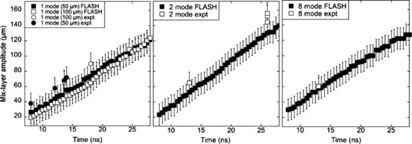
Figure 15. Comparison of FLASH mix-layer amplitude with the (a) one-mode experiment, (b) two-mode experiment, and (c) eight-mode experiment.
Download figure:
Standard image High-resolution image5. BUOYANCY-DRAG MODEL
The growth of the initial perturbation seen in decelerating interface experiments is not entirely due to instabilities. Another significant contributor to mix-layer growth is material expansion. If one hopes to compare the results to simple incompressible models, then it is an important part of data analysis to correct for the mix-layer growth due to material expansion. The following explains how we evaluated the expansion amplitude on the basis of the data and of Hyades simulations.
The amplitude of the mix layer, h, as shown in Figure 11, is a combination of the expansion amplitude, hexp, and the instability amplitude, hinst shown by

Ideally, h from Equation (3) would be the spike or bubble amplitude, which is the difference between the spike or bubble position and the mean interface position from the one-dimensional simulations. However, finding the feature amplitude this way is rather difficult as discussed earlier and instead reference will be made to an overall mix-layer amplitude, half the distance between the spike and bubble.
The expansion amplitude, hexp from Equation (3), is the integral of the velocity of expansion of the mix layer due to the overall expansion of the fluid. This cannot be directly measured from the experiment so a combination of data and one-dimensional simulation results are used. The instantaneous expansion velocity of the spike and bubble is obtained by taking the difference in velocities from the Hyades simulation at the experimental spike-tip or bubble-tip positions. These velocities contain no information about the instability since they are obtained from a one-dimensional simulation. The integral of the instantaneous net expansion velocity results in the net expansion amplitude of the entire mix layer. For the analysis described above the net expansion is divided by 2 to obtain the expansion amplitude, hexp. This analysis was performed separately for the experiments executed using targets with one-mode and two-mode type patterns because experiments using these two types of patterns resulted in the most data. Figure 16 shows the mix-layer amplitude, h, the expansion amplitude, hexp, and the effective incompressible instability amplitude, hinst. The figure indicates that roughly half of the mix-layer growth is due to the instability and half is due to expansion.

Figure 16. Plot of h, half the distance between the spike and bubble, hexp, the amplitude due to expansion, and hinst, the amplitude due to the instability.
Download figure:
Standard image High-resolution imageOnce the material expansion is subtracted from the data a simple, incompressible model for Rayleigh–Taylor mixing, such as the buoyancy-drag model, can be compared to the data. From Oron et al. (2001) and Dimonte (2000) a two-dimensional instability front can be described by
where u is the velocity, g(t) is the acceleration, ρ1 and ρ2 are the post-shock densities of the fluids on either side of the interface. The acceleration of the interface was found from a simulation to be g = −7.5(t/t0)−1.2 and the ratio of the densities is ρ1/ρ2 = 4.26. L is the dynamical length scale of the mixing zone. Dimonte point out that physically L in Equation (4) represents the ratio of volume to cross-sectional area of a single bubble or spike, since volume determines the net buoyant force while area determine drag force. For self-similar multimode turbulence, L, is often related to the wavelength of the dominant bubble. In the present case, it makes more sense to approximate a single spike or bubble as a cylinder (or in the two-dimensional perturbation case, a rectangular prism) so that L becomes the height of the cylinder. Thus, in our case L is the mix-layer amplitude and is now time dependent. It does not depend on the distance between bubbles or spikes. The amplitude changes over time and the expansion corrected data, hinst, was linearly fit to find how the mix-layer amplitude changes with time. This gave a value of 2.72t, where 2.72 is the velocity of amplitude growth in μm ns−1 and t is time in ns, which was used as the length scale in Equation (4). Since the length scale is based only on the available experimental data this analysis is only valid for the time when the experiment was observed, in this case, up to 26 ns. One can see that the dynamical length scale has no dependence on the wavelength of the perturbation only on the amplitude. As all of the patterns have the same amplitude this model predicts that they should all show the same mix-layer amplitude growth. Both the experiments and simulations have shown that the mix-layer amplitude is similar for all cases.
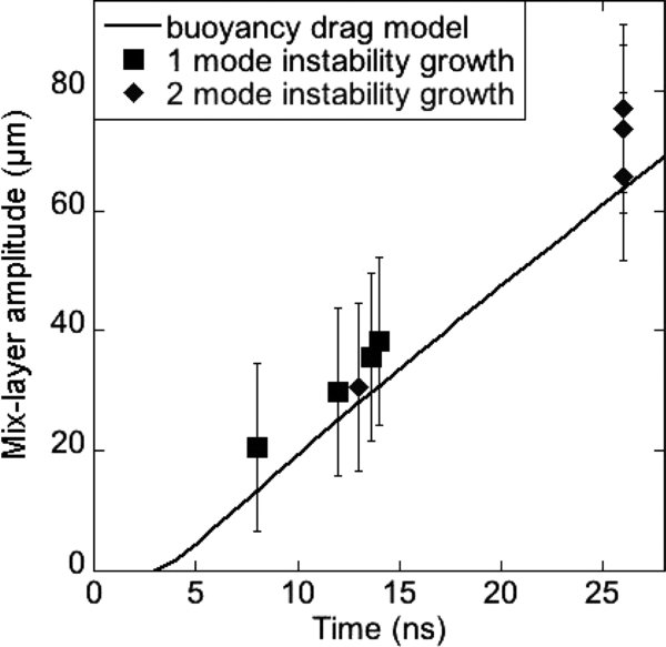
Integrating Equation (4) with respect to time and using results from the Hyades simulations for the initial condition one can solve for the amplitude of the mix layer. The theoretical value of the mix-layer amplitude versus time is shown in Figure 17 along with the inferred hinst for the single- and two-mode type perturbation. The model and experiment are in overall good agreement with the model predicting slightly less growth, but agreeing within the error bars.
Figure 17. Plot of the amplitude vs. time for the (a) single-mode experiments compared to the buoyancy-drag model and (b) plot of the amplitude vs. time for the two-mode experiments and compared to the buoyancy-drag model.
Download figure:
Standard image High-resolution image
6. CONCLUSION
We have presented experiments and simulations relevant to the hydrodynamic processes believed to occurr in SNe. Experiments, dominated by the Rayleigh–Taylor instability, show good agreement with simple, incompressible models. Hydrodynamic simulation results overpredict the shock position, most likely due to the EOS and lateral expansion; yet the results agree within error with experimental mix-layer growth. Further work on hydrodynamic simulations include adjusting the gamma of the foam and polyimide to more accurately predict the shock position. SN relevant experiments are continuing with three-dimensional and more realistic initial conditions.
The authors would like to acknowledge Chuck Source and the Omega operations staff as well as Russell Wallace and the LLNL target fabrication team. The software used in this work was in part developed by the DOE-supported ASC/Alliance Center for Astrophysical Thermonuclear Flashes at the University of Chicago. Financial support for this work included funding from the Stewardship Science Academic Alliances program through DOE Research grant DE FG03-99DP00284, and through DE-FG03-00SF22021 and other grants and contracts.