


ABSTRACT
We examine Advanced Composition Explorer and Helios 1 data in search of evidence for an anisotropic spectrum of interplanetary magnetic and velocity field fluctuations. Specifically, we focus on the power-law indices of the fluctuation spectra and associated second-order structure functions and ask whether the index varies systematically with the angle between the mean magnetic field and the wind velocity. We extend previous results to show convincingly that it does not. Several popular theories for magnetohydrodynamic turbulence predict a significant variation as part of the turbulent cascade dynamic. We offer some observations on why the predicted anisotropy is not present.
Export citation and abstract BibTeX RIS
1. INTRODUCTION
When discussing anisotropy in the interplanetary spectrum at least two different and generally unrelated forms of anisotropy are often considered: the anisotropy in the fluctuation vector (sometimes called the "variance anisotropy" where it is generally the case that more energy resides in fluctuations perpendicular to the mean magnetic field than in parallel fluctuations) and the anisotropy in the underlying wavevector spectrum (where, generally, more energy resides in the wavevectors perpendicular to the mean magnetic field B0 than in those parallel to B0). Unti & Neugebauer (1968), Belcher & Davis (1971), and Klein et al. (1991) have clearly demonstrated the presence of a variance anisotropy. Smith et al. (2006b) attempted to provide partial explanation for this result by noting the correlation between magnetic variance anisotropy and both the plasma β and the magnitude of the inertial range magnetic spectral density. In this paper we explore evidence for one form of anisotropy in the underlying wavevector spectrum: that the power-law index of the spectrum may depend on direction.
The anisotropy of the underlying wavevector spectrum is more difficult to extract than the variance anisotropy using single-spacecraft techniques. This is for two reasons: first, the amplitude of turbulence in the solar wind varies for many reasons, in addition to depending on the direction of the local mean magnetic field; and second, each measured spectrum or correlation function is a reduced quantity that represents an integral over all directions perpendicular to the mean flow. Even if the solar wind were purely homogeneous, the mathematical inversion is difficult and may not be uniquely determined by the data coverage in timescale and angle of magnetic field to solar wind direction. Several schemes have been developed to reveal the wavevector anisotropy in the face of the varying absolute power levels of turbulence in the solar wind, by examining how certain ratios or normalized quantities vary with the direction of the local mean magnetic field.
Matthaeus et al. (1990) offered the so-called "Maltese Cross" result that makes use of rotations in the mean magnetic field to compute correlation functions for magnetic fluctuations as a function of implied spatial separation VSWδt and the angle between the solar wind velocity and mean magnetic field ΘBV. They use 16 months of ISEE-3 data with 15 min resolution that makes use of rotations in the mean magnetic field to plot the reduced correlation function for magnetic fluctuations at 1 AU as computed for large scales (∼7.2 × 10⁵ to 4 × 10⁶ km). They found an admixture of correlation associated with parallel and perpendicular wavevectors with reduced energy levels at intermediate angles to the mean field. Dasso et al. (2005) repeated the analysis using 5 years of 64 s data from the Advanced Composition Explorer (ACE) while separating intervals of fast wind (VSW > 500 km s−1) from slow wind (VSW < 400 km s−1). They focused on slightly smaller spatial scales from 5 × 10⁴ to 1 × 10⁶ km and found two distinct forms in the correlation function with parallel wavevectors dominating the energetics in the fast wind samples and perpendicular wavevectors dominating in the slow wind. Figure 1 shows a model spectrum for turbulence at 1 AU with spatial scales of the above studies marked.

Figure 1. Solid line: model interplanetary spectrum for 1 AU. Break in spectrum is the approximate correlation scale. Onset of dissipation scale at ∼0.3 Hz is omitted. Short dash: estimate of τnl derived from the spectrum. Long dash: estimate of τA assuming VA = 40 km s−1. Lifetime of solar wind from Sun to 1 AU (horizontal arrow). Corresponding spatial/temporal scale in the spectrum matches the approximate correlation scale of the turbulence (vertical arrow). The scale for k relates to the radial component only, kR, and assumes VSW = 400 km s−1.
Download figure:
Standard image High-resolution imageBieber et al. (1996) employed several direct methods to determine the fraction of total energy that resides in perpendicular (two-dimensional) wavevector modes and in parallel (slab) wavevector modes using single-spacecraft measurements. These methods rely on the assumption that the turbulence is axisymmetric about the mean magnetic field. In their "spectrum ratio" test they use the theory of correlation functions in a turbulent fluid and neatly remove the effect of varying absolute power. They study Helios observations selected to occur just before and during 29 solar energetic particle events (Wanner 1993) using 454 intervals lasting 34 minutes each and focus on scales from 49 to 1020 s (1.96 × 10⁴ to 4.08 × 10⁵ km assuming a wind speed of 400 km s−1). They find that on average 85% of the energy resides in the two-dimensional component while only 15% of the energy is associated with parallel wavevectors. Leamon et al. (1998) use 33 one-hour samples of (Wind) magnetic field data and extend this result to the high-frequency end of the inertial range. They find on average 89% of the energy associated with the two-dimensional component. Hamilton et al. (2008) separate fast and slow winds in a study using 960 intervals of ACE data recorded from 1998 through 2002 and find no significant difference between fast and slow wind samples at the smallest scales of the inertial range.
When there is an anisotropy in the power level of the underlying spectrum it is natural to expect there may be an anisotropy in the associated spectral indices. If for no other reason, the spectrum S(k) should be continuous (although it is often modeled as a discontinuous function) and must be the same as k → 0 from any direction. Therefore, at some scale differing power levels must reflect different spectral forms. Sari & Valley (1976) examine spectra from 16 intervals of magnetic field measurements by Pioneer 6 over the frequency range 4 × 10⁻⁴ to 1.6 × 10⁻² Hz. Eight intervals have nearly radial mean magnetic fields and eight have azimuthal mean fields. No significant differences in spectral index are reported. Bavassano et al. (1982) offer similar analyses of 72 spectra computed from Helios magnetic field observations inside 1 AU with similar conclusions. Other authors have provided similar results with equally small sample size. The theories reviewed in the next section make specific predictions for the anisotropy of the spectral index that we examine using 10 years of observations by the ACE spacecraft and additional observations by Helios 1.
In Section 2, of this paper we review developments in magnetohydrodynamic (MHD) turbulence theory that attempt to describe the spectrum that would be seen by a single spacecraft for varying ΘBV. In Section 3.1, we introduce a data analysis scheme that uses the index of second-order structure functions as a proxy for the index of power spectra to study the observed mean spectral indices seen in the solar wind as a function of ΘBV. This constitutes an analysis of 1 to 10 min (2.4 × 10⁴ to 2.4 × 10⁵ km) oscillations in the ACE magnetic field and solar wind velocity data recorded at 1 AU. In Section 3.2, we examine power spectra from within a known database of magnetic spectra computed from ACE observations spanning 10 to 100 s (4 × 10³ to 4 × 10⁴ km). In Section 3.3 we repeat the ACE high-frequency analysis using Helios 1 magnetic field measurements from 50 to 200 s (2 × 10⁴ to 8 × 10⁴ km) recorded from 0.3 to 1 AU. We close by summarizing our results.
2. THEORY OF ANISOTROPIC MHD
There is significant evidence to suggest the observed distribution of energy between quasi-parallel and quasi-perpendicular wavevectors is the result of the natural evolution of MHD turbulence. Experiments using liquid metals (collision-dominated MHD fluids) with an applied DC magnetic field show the turbulence evolves to nearly two-dimensional flow confined to the plane perpendicular to the applied DC field (Lielausis 1975; Tsinober 1975; Volish & Kolesnikov 1976). Likewise, Macrotor tokamak and Zeta-Pinch experiments (plasma MHD systems) have shown two-dimensional geometries in the presence of a strong DC magnetic field (Robinson & Rusbridge 1971; Zweben et al. 1979). MHD simulations by Shebalin et al. (1983), Ghosh et al. (1998), Oughton et al. (1994), Matthaeus et al. (1996), and Cho & Vishniac (2000) and Hall–MHD simulations by Ghosh & Goldstein (1997) have shown that energy in inertial range fluctuations moves to perpendicular wavevectors in the presence of a mean magnetic field. However, a theory that predicts the spectral form of the fluctuations is slow to develop.
At the heart of the problem is the fact that MHD turbulence in the presence of a mean magnetic field exhibits two distinct characteristic timescales. The first is the eddy turnover time τnl(k) ≡ 1/(kuk) where uk is the characteristic speed at scale 1/k, which we write as  for the omnidirectional spectrum
  , which satisfies
  . The second is the Alfvén wave propagation period τA(k) ≡ 1/(k∥VA) where VA is the Alfvén speed
  . Figure 1 plots values for τnl (assuming isotropy and using the model spectrum shown) and τA (assuming k∥ = k and VA = 40 km s−1). For small k∥ compared with k, however, τA will be larger.
In traditional hydrodynamics there is only the eddy turnover time. From τnl and the assumption of local interactions Kolmogorov (1941) predicted that the omnidirectional spectrum of isotropic turbulence would behave as Ek ∼ k−5/3. This same argument is extended to include two-dimensional MHD (Fyfe et al. 1977; Montgomery & Turner 1981; Montgomery 1982, 1989).
Reduced magnetohydrodynamics (RMHD) is an attempt to bring wave dynamics into the scaling of turbulence and address the quasi-parallel wavevector component. Montgomery & Turner (1981) and Montgomery (1982, 1989) conclude that the RMHD component of the spectrum should fall off rapidly in the k∥ direction. Higdon (1984) argues that the marginal condition where the Alfvén time equals the nonlinear time in the inertial range gives a relationship between the parallel and perpendicular wavenumbers of the form k∥ ∼ k2/3⊥. Later Goldreich & Sridhar (1995) develop an example built on the above ideas in the context of the eddy damped quasinormal Markovian approximation (EDQNMA) that we revisit below.
RMHD is the form of nonlinear quasi-two-dimensional MHD that continues to have O(1) timescales and strong nonlinear interactions even as the frequency of Alfvén waves formally approaches infinity. The marginal condition for the perturbative derivation of RMHD is that the Alfvén wave period τA = 1/(k∥VA) is equated with the scale-dependent eddy turnover time τnl(k) = 1/(kuk). This is what Goldreich & Sridhar (1995) term "critical balance." We assume a Kolmogorov spectrum  and that the decay rate is vonKarman in form (
 = u3/L where u is the rms speed or turbulence amplitude). After some simple rearrangement the marginal condition τnl = τA becomes
where we employ the additional assumption that the anisotropy is so strong that k ≈ k⊥ + O(u/VA), thus justifying writing k⊥ on the right-hand side. This boundary is shown in Figure 2.
Figure 2. Depiction of Goldreich & Sridhar (1995) contour under "critical balance" assumption. Vertical hashed lines denote integration over perpendicular wavevector components to yield measured spectrum of reduced wavevectors parallel to mean magnetic field. Figure shows regions of dominant τA and τnl.
Download figure:
Standard image High-resolution imageFor the limited purpose of this paper, and acknowledging that this definition may be at odds with the usual conventions used in observational space physics, we define quasi-parallel (quasi-perpendicular) wavevectors to be those wavevectors on the large-k∥ (large-k⊥) side of the boundary given by τnl = τA. This does not require that the angle between the k∥ axis and the quasi-parallel wavevector is small, but only that it lies on the large-k∥ side of the boundary. With this definition we can assert dynamics which are associated with the two distinct sides of the boundary.
For quasi-perpendicular wavevectors, steady nonlinear effects dominate over wave propagation effects, and a Kolmogorov-like spectrum is expected (as assumed already in Equation (1)). However there is no guarantee that the incompressible RMHD cascade is the only element that may be present in a real instance of plasma turbulence: for quasi-parallel wavevectors, wave-like time variations may be more effective than nonlinear couplings, but various factors including the method of driving, initial or boundary conditions, large-scale instability, or wave–particle interactions may sometimes introduce fluctuations having k∥ larger in magnitude than the marginal Equation (1) value. However even for quasi-parallel wavevectors the resonant nonlinear couplings described by Shebalin et al. (1983) and Oughton et al. (1994) may be dominant. We would like to emphasize that the existence of this boundary and of a strongly turbulent RMHD region of wavenumber space, does not imply that wave-like or resonantly coupled high-frequency MHD turbulence cannot exist within the quasi-parallel wave-vector region. In the following subsection we examine and test some observational consequences of the assumption that power at finite τA (=non-zero k∥) scales as indicated by Equation (1).
2.1. Goldreich & Sridhar Model Spectrum
Goldreich & Sridhar (1995) adopt a particular form of the RMHD spectrum. They assume that perpendicular spectral transfer is governed by triple correlations that decay at the nonlinear timescale τnl(k). Under this assumption of a high degree of anistropy of the type discussed by Shebalin et al. (1983) this timescale depends only on the perpendicular wavenumber k⊥ and parallel transfer is fully suppressed. Building these assumptions into an EDQNMA closure calculation, Goldreich & Sridhar (1995) write a steady model spectral density as
where a is a dimensionless number. The fluctuations are assumed small compared to the mean field, δB/B0 ≪ 1, and the energy-containing length scale is L. The dimensionless function f(ξ) has the property that ∫+∞−∞f(ξ) dξ = 1. In keeping with the critical balance separation of timescales, the reduced spectrum along any line with k∥ = 0 has an infinite Alfvén time and is thus assumed to have the Kolmogorov k−5/3⊥ form resulting from τnl dynamics. At any k with non-zero k∥, however, the three-dimensional spectrum is assumed to scale as some function of τnl/τA ∝ k∥L1/3/k2/3⊥. The three-dimensional spectrum Equation (2) combines these two assumptions in a general form whose implications can be described and tested, which we now proceed to do.
Integration over the parallel wavenumber kz yields a "Kolmogorov" spectrum in perpendicular wavenumber
The two-dimensional model spectrum has dimensions EL2 and one obtains the two-dimensional omnidirectional spectrum from it by integrating over angle, i.e., multiplying by 2πk⊥ as axisymmetry is assumed. Therefore  as expected.
If we integrate the model spectrum over the two k⊥ directions, we obtain a one-dimensional reduced spectrum that depends on kz. This is the spectrum that would be observed if the mean magnetic field of the solar wind were radial with the mean super-Alfvénic flow in the same radial direction. The observed (or "reduced") spectrum is
Letting k'⊥ = k⊥L and q = k∥L/k2/3⊥ the above integral involves
The reduced spectrum is then given by
where a' = a∫∞0dqqf(q). Therefore, following the arguments of RMHD and the critical balance assumption, energy is largely absent from quasi-parallel wavevectors due to nonlinear coupling that transports the energy to larger k⊥. If these arguments apply and under the frozen-in-flow approximation, one expects the observed spectra to approach f−2 as ΘBV → 0°.
We now consider the effect of a sharp cutoff in the spectrum at small scales, say at the ion inertial scale wavenumber kii = ωpi/c = Ωci/VA. The observed inertial range of interplanetary magnetic fluctuations is seen to possess a strong spectral break associated with the ion inertial scale, although this normally marks a transition to a steeper power-law form (Leamon et al. 1998; Smith et al. 2001; Hamilton et al. 2008). For simplicity of this demonstration we assume here that E(k⊥, k∥) = 0 for k⊥ > kii. This sharp cutoff implies also a cutoff in the reduced spectrum computed above. Using Equation (1) we conclude that the observed spectral density reduced over the two perpendicular directions will cutoff sharply at a parallel wavenumber k∥ ∼ kd∥ where
The second form of the right-hand side emphasizes that the cutoff wavenumber scales as δb/B0 (assuming approximate equipartition of magnetic and velocity field turbulence energies) and also that the cutoff depends on the ion inertial scale (assuming that the perpendicular dissipation or steepening scale is of this order). Note that the cutoff in k∥ will be less sharp in all cases in which the kinetic steepening range in the perpendicular direction is less steep than the extreme case considered here. This demonstrates that there should be a change in the spectral slope to steeper than f−2 at the above parallel wavenumber kd∥ when the reduced spectrum is computed along the mean magnetic field.
We note that the above analysis applies to inertial range scales only. We have described the expected cutoff at large k due to dissipation in the Higdon (1984) and Goldreich & Sridhar (1995) theory noting that the observed cutoff kd∥ (kd⊥) in the parallel (perpendicular) directions is highly anisotropic with kd∥ ≪ kd⊥. The inertial range also does not extend to k = 0; there is expected to be an energy-containing range at larger scales associated with boundary data or driving that is not yet processed by the in situ turbulent cascade. We assume that the termination of the inertial range at large scales occurs at a wavenumber k ∼ 1/LC with LC the correlation scale. Combining these ideas we can create Figure 2 to demonstrate both the computed separatrix between τnl- and τA-dominated regions of the spectrum. The vertical hatched bars represent the integration necessary to compute the parallel spectrum. Note how this integration spans both regions of quasi-perpendicular wavevectors dominated by τnl and quasi-parallel wavevectors where, if the Goldreich & Sridhar (1995) model spectrum correctly and completely describes the turbulence, no additional fluctuation power should exist.
3. DATA ANALYSIS
Turbulence in the solar wind at Earth's orbit (1 AU and solar equatorial latitude) has been shown to exhibit a strong collapse to the two-dimensional state with quasi-perpendicular wavevectors dominating the energy spectrum (Matthaeus et al. 1990; Bieber et al. 1996; Leamon et al. 1998; Dasso et al. 2005; Hamilton et al. 2008). The dynamic cascade toward the two-dimensional state has now been measured directly (MacBride et al. 2008). It therefore seems reasonable to search for evidence of the Higdon (1984) and Goldreich & Sridhar (1995) prediction of a critical balance boundary in k-space as evidenced by spectral steepening of the measured power spectrum when the mean magnetic field is aligned with the mean wind velocity. In the process, we can ask whether the measured spectral indices are dependent in any manner on their orientation relative to the mean magnetic field as general axisymmetric turbulence ideas would suggest the spectrum may be.
We have employed traditional analysis methods to study three separate datasets where each dataset is selected for a different reason. In the first instance we use second-order structure functions to infer spectral indices for power spectra without the need to compute the spectra directly. We apply this technique to a merged dataset of magnetic field and thermal ion data recorded by the ACE spacecraft at 1 AU with 64 s resolution and obtain estimates for the spectral index over a frequency range from 1.6 to 16 mHz. In the second instance we compute power spectra from 960 hand-picked intervals of high-resolution (3 vector s−1) magnetic field data recorded by the same spacecraft and examine the spectral indices in the range 10 mHz to 0.2 Hz. In the last instance we examine magnetic field spectra computed from 380 hand-picked intervals recorded by the Helios 1 spacecraft from 0.3 to 1 AU during solar minimum conditions using 6 vector s−1 data and focus on frequencies from 5 to 20 mHz. In each instance we examine the statistics of spectral indices as a function of ΘBR, the angle between the mean magnetic field and the radial direction from the Sun to the spacecraft (taken to be the direction of the solar wind flow).
3.1. ACE 64 s Merged Data
We examine ACE data from day 23 of 1998 through day 56 of 2007. This period spans both solar maximum and solar minimum conditions. We use the merged dataset of thermal ion and magnetic field measurements recorded by the SWEPAM and MAG instruments (McComas et al. 1998; Smith et al. 1998). The data have 64 s resolution because this is the collection rate of the SWEPAM instrument. MAG data are averaged to the same time resolution in a manner that is syncronized to the data collection times of SWEPAM in producing this merged dataset.
The data are recorded in RTN coordinates (R is the radial direction from the Sun to the spacecraft, T is the azimuthal direction coplanar with the Sun's equatorial plane and directed in the sense of rotation, and N is the normal such that R × T = N). The solar wind flows in the +R direction, unless deflected by stream interaction, ejecta, or planetary magnetospheres. Systematic excursions of the wind velocity away from the radial direction are minimal except for the fluctuations that constitute the turbulence. When measurements are recorded within or near the Sun's equatorial plane, as they are here, the N component is directed northward. This has certain advantages as we shall see below.
We take 1 hr intervals of the merged data and perform several tasks: (1) we compute means and uncertainties for each component of the magnetic field and solar wind vector in RTN coordinates; (2) we perform a linear detrend of the data interval in anticipation of obtaining computed variances that are consistent with first-order structure function statistics; (3) we compute variances and uncertainties for each component of the magnetic field and solar wind vector in RTN coordinates; (4) we compute second-order structure functions for each component of the magnetic vector for lags from 1 to 10 points (64 to 640 s), then sum to obtain the trace of the magnetic structure function matrix; (5) we do the same for velocity vectors; and (6) we fit the structure functions for each hour (amplitude and power-law index with uncertainties) assuming a power-law form. This results in ∼74, 000 independent intervals used in this analysis.
The second-order structure function S2(L) of a variable Z(x) measured at positions x is defined to be

where 〈 ⋅ ⋅ ⋅ 〉 denotes ensemble average. It is common to replace the ensemble average with an average over the data interval and we assume that S2 is not a function of x. It is then possible to compute the power spectrum of the same time series by transforming S2 (Smith et al. 1990). However, one can infer directly the spectral index q of the resulting power spectrum (in the sense that the spectrum varies as kq) if S2(L) ∼ ALn according to q = −(n + 1). We may therefore fit the computed estimates for S2 and infer a spectral index together with uncertainty without computing the power spectrum directly.
Figure 3 shows the distribution of computed structure function indices for four measured variables used in this study: the trace of the second-order structure functions for the magnetic vector, the velocity vector, the N component of the magnetic vector, and the N component of the solar wind velocity. We include the statistics for BN because this component is relatively free of current sheet crossings, which can contaminate the analysis of individual samples. We include the statistics for VN because variation in wind speed over an hour, as seen in VR, can dominate the trace analysis for some intervals whereas VN is largely only a fluctuation due to the turbulence and lacks these large-scale trends. We further subset the data into slow wind (VSW < 400 km s−1) and fast wind (VSW > 500 km s−1) in the manner of Dasso et al. (2005) in addition to using all wind conditions. These subsets are based on the mean wind speed for the hour. Several things become readily apparent: first, the most probable structure function index for the magnetic field measurements (both trace and BN) is centered near 2/3 whereas the most probably index for velocity measurements (also both trace and VN) is centered near 1/2. In fact, the latter is more nearly 0.4 as we shall see. A structure function index n = 2/3 implies a spectral index q = −5/3 while n = 1/2 is consistent with q = −3/2. Podesta et al. (2006, 2007) report a velocity spectra index that is approximately −3/2 at 1 AU and −3/2 is a prominent prediction in MHD turbulence theory (Kraichnan 1965). Second, the statistics for the N-component fluctuations are in good agreement with the trace values, suggesting that concerns over possible contamination by objects such as current sheet crossings are unwarranted at this level. Third, values of n = 1 implying q = −2 are less common, but not unrepresented in the dataset. Fourth, there is a systematic variation in the fit indices for fast and slow winds in both magnetic and velocity measurements that is beyond the scope of this analysis. Fifth, there are a finite number of events with indices n ∼ 0 implying q ∼ −1, but flatter spectra are not found.
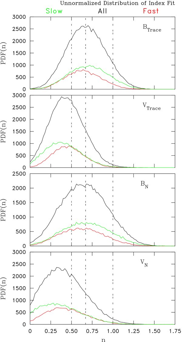
Figure 3. Analysis using ACE data from 1998–2007 with 1 hr intervals and 64 s resolution. Statistics for fast, slow, and all winds are shown. Top panel shows distribution of fitted power-law indices for trace of B tensor. Middle panel shows distribution of indices for trace of V tensor. Bottom panel shows distribution of indices for north–south component of B. Vertical dashed lines mark n = 0.5, 0.67, and 1.0 (q = −1.5, −5/3, and −2, respectively.)
Download figure:
Standard image High-resolution imageBefore proceeding to the ΘBR dependence we compute the distribution functions for the standard deviations in the fit indices. These are shown in Figure 4. The key feature is that the uncertainties are generally several times smaller in comparison with the fitted means with most probable values of the uncertainties ⩽0.1. This suggests that fit indices are generally well determined and is a necessary condition to obtaining good statistics in the next stage of the analysis.
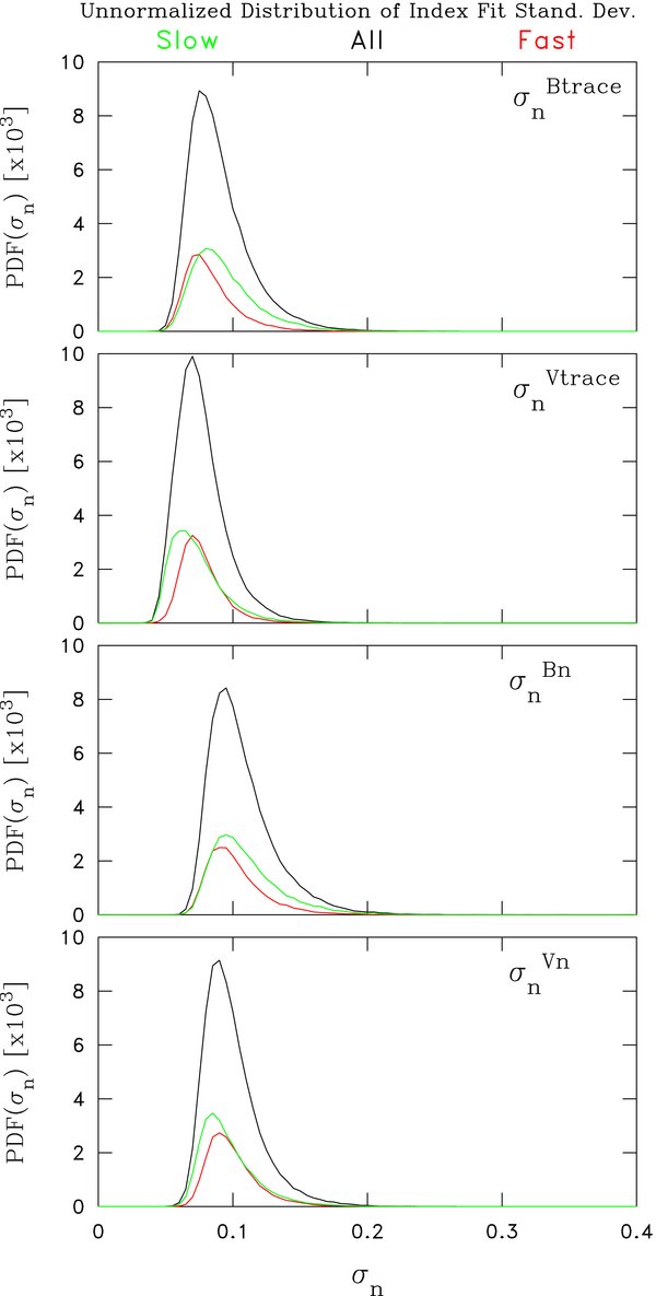
Figure 4. Same as Figure 3 showing distribution of computed uncertainties in power-law indices for each fitted interval.
Download figure:
Standard image High-resolution imageFrom this point on we compute error-weighted means according to the prescription
where ni is an individual fit index and σi is the error associated with the fit. We can then compute the variance of the associated distribution
with σstdev being the standard deviation. Since there are two sources of error, the individual measurement error and the computed width of the distribution which may arise from many other sources and reflect the natural variation of the parameters, we define the error-of-the-mean σerr according to

where N is the number of hourly fits. Each ΘBR bin shown in subsequent plots contains several hundred to several thousand independent estimates of the index, so the computed error-of-the-mean for each binned quantity is considerably smaller than the symbols used in plotting.
Since the widths of the distributions in Figure 3 are greater than the most probable value of the fit uncertainties in Figure 4, we assume there is a natural variation to the distribution of n apart from simple measurement error. This is the motivation for the above definition of σ2err. We will use standard deviations when plotting uncertainties unless otherwise stated to reflect the broad distribution of values that underly each mean. We do this to demonstrate that spectra with −2 indices are more than one standard deviation off the mean of the distribution, which is an indication that it is relatively rare. If we assume there is a single universal theory governing the distribution of n, then it would be appropriate to compare −2 indices with the error-of-the-mean. As we accumulate estimates the error-of-the-mean becomes progressively smaller and the −2 spectra become an increasing number of uncertainties from the mean, but its occurrence rate in the distribution does not change. Readers are left to ponder which interpretation they favor.
Figure 5 shows the computed average indices according to the above error analysis gathered into 5° bins of the variable ΘBR. As stated, error bars again represent the computed standard deviation. No statistically significant dependence on ΘBR is seen in any of the four panels. In each case the mean value of the S2 index is consistent with the most probable values shown in Figure 3. The computed standard deviations in all ΘBR bins are comparable to the width of the distribution shown in Figure 3. This means that the predicted structure function index 1, or equivalently the spectral index −2, is consistently more than one standard deviations from the mean for all values of ΘBR.

Figure 5. Same analysis as Figure 3, but accumulating mean and variances for fitted power-law indices as a function of ΘBR.
Download figure:
Standard image High-resolution imageCoverage in each bin varies according to ΘBR and the quantity in question. For instance, the BTrace distribution for 40° < ΘBR < 45° contains 5793 estimates of ni. The computed 〈ni〉 is 0.674 while the computed standard deviation is 0.219 and the error of the mean is 0.003. For the bin 0° < ΘBR < 5° there are 384 estimates of ni. The computed 〈ni〉 = 0.702 while the computed standard deviation is 0.22 and the error-of-the-mean is 0.01. If the Goldreich & Sridhar (1995) theory is an occasional truth under carefully prescribed conditions, then its occurrence rate is 1.4 standard deviations from the mean. If it is proposed as a universal theory of MHD turbulence, then its occurrence rate is 30 error estimates from the mean.
It is reported that the wavelet methods of Horbury et al. (2007) better resolve the expected low-amplitude spectra anticipated for the small-ΘBR spectrum. While this is less of a problem for low-latitude measurements at 1 AU than for the high-latitude Ulysses measurements used by Horbury et al. (2007), since δB/B0 is smaller in the ACE dataset than for Ulysses measurements, we can address the possibility by limiting our analysis to those intervals with low fluctuation levels so that the instantaneous magnetic field remains within the assigned ΘBR range. This is also beneficial to comparison with the Goldreich & Sridhar (1995) prediction that is based on the assumption that the mean field is much larger than the fluctuations. To do this, we define ΘB ≡ arctan(B⊥,rms/|B0|) where B⊥,rms is the root-mean-square variation of the component of the magnetic field perpendicular to the mean field direction. In this way ΘB becomes a measure of the variability of the field direction and intervals with both small ΘBR and small ΘB can be inferred to sample the τA-dominated region of the spectrum without contamination from the τnl-dominated portion of the spectrum.
Figure 6 shows the resulting mean values of n and q when ΘB is limited to less than 30°, less than 15°, and less than 5°. To leading order the computed standard deviations do not change with decreasing ΘB. There is, in fact, a slight decrease in the standard deviations as ΘB is made small. In the interest of full disclosure, there are only nine intervals for ΘBR < 10° and ΘB < 5°. However, their spectra fail to show any trend toward n = 1 or q = −2. The spectral index of magnetic fluctuations continues to be ∼−5/3 and for velocity fluctuations ∼−1.4 for all values of ΘBR. There is no evidence of spectral indices q = −2 associated with small ΘBR.

Figure 6. Same analysis as Figure 5, but limiting samples to those hours when ΘB< prescribed angles.
Download figure:
Standard image High-resolution image3.2. ACE High-Resolution MAG Data
Hamilton et al. (2008) argue that small-scale fluctuations within the inertial range evolve more rapidly than large-scale fluctuations as a result of the arguments put forward by Kolmogorov (1941) and his assumption that cascade dynamics are local. In an effort to extend these results to smaller spatial scales (higher frequencies) we examine the database used by Smith et al. (2005, 2006a, 2006b) and Hamilton et al. (2005, 2008). This database is built on five years of ACE observations spanning 1998 through 2002 and includes 960 data intervals with 393 intervals from 28 distinct magnetic clouds. Data intervals are from 1 to 3 hr in duration and nonoverlapping. A complete description of the spectral analysis technique and the resulting database parameters is provided in the above references. Unlike the above analysis, we now focus on the fitted results of power spectra and not the inferred spectral characteristics derived from second-order structure functions. The database uses 3 vector s−1 magnetic field data and we focus on frequencies at the high end of the inertial range (typically from 8 mHz to 0.1 Hz). The exact frequency range varies with individual data intervals so as to remain at frequencies smaller than the spectral break and larger than any poorly resolved spectral features that depart significantly from power law. Typically, any such variation in the frequency interval is small.
Figure 7 shows the results of this analysis. The trace of the magnetic power spectral matrix (the spectrum of total power in the magnetic fluctuation) is computed and the spectral index is fitted over the above frequency interval. The indices are averaged in 10° bins of ΘBR using the same uncertainty-weighted averaging scheme described above. Uncertainties on the plot are again representations of the standard deviation of the underlying distribution. Errors-of-the-means are several to ten times smaller than the standard deviations. As before, the database is subsetted for fast and slow winds of open field conditions and to this we add the above subset of magnetic cloud observations. Results for ΘBR ⩾ 30° seem perfectly consistent with −5/3 indices seen above. The 20° ⩽ ΘBR < 30° bin for fast winds and the 0° ⩽ ΘBR < 10° bin for slow winds may constitute anomalous results due to poor coverage. For ΘBR < 30° there is some degradation of the results, but no evidence of a trend toward a −2 spectral index. In fact, the cloud set clearly shows a small angle trend toward a flatter than normal spectrum.
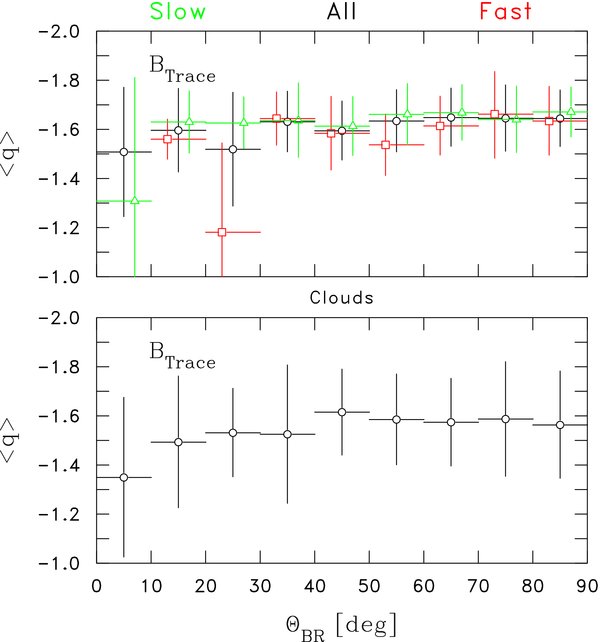
Figure 7. Accumulating mean and variances for fitted power-law indices as a function of ΘBR for magnetic trace spectra using the Hamilton database. Top: mean indices for all open field line (black), fast wind open field lines (red), and slow wind open field lines (green). Bottom: mean indices for all cloud observations.
Download figure:
Standard image High-resolution imageTo summarize the analysis using the high time resolution dataset, there is no evidence of a trend toward −2 spectral indices at any value of ΘBR. Furthermore, this is strong evidence against steepening to spectral indices steeper than −2 that would be due to projection of a perpendicular range cutoff as described by Equation (7).
We should note that despite using 960 data intervals in this analysis, only 23 intervals of open field lines fell in the range ΘBR < 20° and no intervals of fast wind fell in ΘBR < 10°. Cloud results were much more likely to exhibit radial mean initial mass function (IMF) conditions. We attempted to increase the number of radial IMF intervals by examining the years 2003–2006 (solar minimum conditions), but found that virtually every interval selected was contaminated by upstream waves from Earth. We do not believe that any existing intervals suffer from this contamination, but most of those additional events selected from solar minimum conditions for possible incorporation into the database were contaminated. We were left with little alternative but to examine data from locations far beyond the Earth–Sun line.
3.3. Helios 1 MAG Data
To escape the possible contamination of the analysis in Section 3.2 by upstream waves and to extend the range of validity of our conclusions to include measurements recorded closer to the Sun where the solar wind turbulence is less evolved, we now examine 380 intervals of IMF spectra measured by the Helios 1 spacecraft in the range 0.3 < RHelios < 1 AU during the years 1974–1976. Intervals are typically several hours in duration and we again employ the same analysis method as used in Section 3.2. We limit our analysis to the frequency range 5 to 20 mHz, which is generally in the middle of the inertial range spectrum. As with the above analysis, every effort was made to cover the broadest possible range of solar wind conditions made available in these years.
Figure 8 shows the results of our analysis. As above, we find no evidence of a consistent shift in the spectral index toward −2 or any steepening of the spectrum associated with nearly radial mean field conditions. Instead, there appears to be a general flattening of the spectrum associated with radial mean field conditions ΘBR < 40°. To the extent that a greater number of radial events may be found at smaller heliocentric distances, this general trend is reported by Bavassano et al. (1982) where it is shown that the inertial range spectrum of interplanetary magnetic field fluctuations steepens with increasing heliocentric distance from 0.3 to 1 AU. Additionally, our analysis shows that fast wind spectra are generally flatter than slow winds. The distribution of indices as a function of ΘBR over the range 0.3 < RHelios < 0.4 AU is statistically equivalent to what is shown in Figure 8. Nowhere in the Helios dataset do we find evidence for −2 spectra in association with radial mean magnetic fields.
Figure 8. Same as top panel in Figure 5 except using Helios 1 magnetic field data over the range 0.3 < RHelios < 1.0 AU spanning the years 1974–1976 for frequencies 5–20 mHz.
Download figure:
Standard image High-resolution image
4. DISCUSSION
Our efforts to find evidence of a measured power spectral index dependent upon the orientation of the mean magnetic field have confirmed the conclusions of Podesta et al. (2006, 2007) who find that the velocity spectral index at 1 AU is more nearly −3/2 than −5/3 and we find no dependence of this result upon the orientation of the mean magnetic field. Specifically, we find the velocity spectra center on a −1.4 spectral index with an error-of-the-mean that makes this result distinct from −3/2. However, the standard deviation is such that −3/2 is well within the range of credible interpretations and as a general statement for the spectral characteristics at 1 AU we are unable to determine whether the velocity spectrum is consistent with Kraichnan (1965) dynamics or coincidental for other reasons. Roberts (2007) argues that the velocity spectrum evolves to have a −5/3 index by 5 AU. The velocity result remains unexplained and points to likely solar wind source dynamics for resolution.
We have examined the conclusion drawn from Goldreich & Sridhar (1995) that measured spectral indices of magnetic and velocity spectra when the mean magnetic field is nearly radial will approach −2 and steeper values and find no evidence of this in either the ACE or Helios data. Nowhere in our presentation do we argue that spectra with −2 indices are unobserved. In fact, Figure 3 clearly shows that such results can be found. Each of the analyses presented here reveals that such events are possible, if infrequent. What we find is that there is no consistent trend toward −2 spectra associated with radial mean fields and that −2 spectra are no more common under radial IMF conditions than for any other orientation of the mean IMF. They are, in general, more than one standard deviation from the mean of the distribution across all orientations of the mean IMF. As a prediction for a potentially universal theory of turbulence, the −2 spectra are many errors-of-the-mean removed from the mean spectral index. The question before us would seem to be "Under what circumstances can we reliably find −2 spectra and is this the result of MHD turbulence or some other interplanetary process?"
The Goldreich & Sridhar (1995) theory descends from the assumption of a strong and well defined mean magnetic field where δB/B0 is small. We take δB to be the characteristic fluctuation for a given scale size, in which case inertial range fluctuations at 1 AU generally satisfy this restriction reasonably well considering that a precise prescription for "small" is not available. However, we are sensitive to this issue. This is one of several reasons why we have examined the small-ΘB limit shown in Figure 6. Still, even then we find no evidence for a consistent −2 spectrum at small ΘBR.
What is most striking in this analysis is the reproducibility of a single spectral index for all values of ΘBR. Magnetic and velocity spectra differ, but their spectral indices do not vary with ΘBR. This seems to suggest that the quasi-parallel and quasi-perpendicular wavevectors remain sufficiently coupled to a common dynamic that they share identical spectral forms. How this can occur within the RMHD formulation, or even why it should be the case, has yet to be shown.
5. SUMMARY
We have examined data recorded by the ACE spacecraft at 1 AU and the Helios 1 spacecraft as it journeyed from 0.3 to 1 AU. We have focused on fluctuations with 640 s spacecraft frame periods and smaller. We verify the Podesta et al. (2006, 2007) conclusions that the velocity fluctuations possess a shallower spectrum than the magnetic fluctuations and have a mean spectral index of −1.4. The magnetic spectra possess an average index of −5/3.
We have systematically explored the spectral index as a function of the angle between the mean magnetic field and average flow velocity and find no evidence for the −2 spectral index predicted by Goldreich & Sridhar (1995). This may not be surprising. MacBride et al. (2008) demonstrate that the turbulent cascade at 1 AU is active in both the perpendicular and parallel directions with the perpendicular cascade dominating. A pure RMHD model, as well as the particular case of Goldreich & Sridhar (1995), assume that the cascade is completely dominated by low-frequency modes with wavevectors almost perpendicular to the mean field. While such turbulence may be energetically important, there is also published evidence in spectral analysis (Bieber et al. 1996) and in particle scattering observations (Bieber et al. 1994) that seem to require that a non-negligible component of the turbulence lies in modes on the k∥ side of the RMHD boundary that may even be in quasi-parallel wavevectors. The present study may be regarded as a further direct test of the idea espoused in the Goldreich & Sridhar (1995) theory—that RMHD modes are a complete representation of the turbulence. This seems not to be the case in the solar wind, at and within 1 AU. However, additional study would be needed to evaluate this possibility as the system evolves further out in the heliosphere, or at high latitudes.
The authors thank the ACE/SWEPAM team for providing the thermal proton data used in this study. J.A.T., B.T.M., and C.W.S. are funded by Caltech subcontract 44A-1062037 to the University of New Hampshire in support of the ACE/MAG instrument. C.W.S. and M.A.F. are supported by NASA Sun–Earth Connection Guest Investigator grant NNX08AJ19G. J.A.T., C.W.S., and J.E.B. are supported by NASA grants NNH04AA17I (RSSW@1AU), NNH06AD52I (Solar & Heliospheric SR&T), and NNG05HL43I (Sun–Earth Connection GI). W.H.M. acknowledges support of National Science Foundation (NSF) ATM-0539995, ATM-0752135 (SHINE) and NASA NNX08AI47G (Heliophysics Theory). J.A.T. is an undergraduate physics major at the University of New Hampshire. B.T.M. was an undergraduate at UNH when he constructed the Helios database used here and he is now a graduate student at UC/Berkeley. We acknowledge helpful discussions with B. J. Vasquez.