


ABSTRACT
We present an analysis of stellar populations and evolutionary history of galaxies in three similarly rich galaxy clusters MS0451.6−0305 (z = 0.54), RXJ0152.7−1357 (z = 0.83), and RXJ1226.9+3332 (z = 0.89). Our analysis is based on high signal-to-noise ground-based optical spectroscopy and Hubble Space Telescope imaging for a total of 17–34 members in each cluster. Using the dynamical masses together with the effective radii and the velocity dispersions, we find no indication of evolution of sizes or velocity dispersions with redshift at a given galaxy mass. We establish the Fundamental Plane (FP) and scaling relations between absorption line indices and velocity dispersions. We confirm that the FP is steeper at z ≈ 0.86 compared to the low-redshift FP, indicating that under the assumption of passive evolution the formation redshift, zform, depends on the galaxy velocity dispersion (or alternatively mass). At a velocity dispersion of σ = 125 km s−1 (Mass = 1010.55 M☉) we find zform = 1.24 ± 0.05, while at σ = 225 km s−1 (Mass = 1011.36 M☉) the formation redshift is zform = 1.95+0.3−0.2, for a Salpeter initial mass function. The three clusters follow similar scaling relations between absorption line indices and velocity dispersions as those found for low-redshift galaxies. The zero point offsets for the Balmer lines depend on cluster redshifts. However, the offsets indicate a slower evolution, and therefore higher formation redshift, than the zero point differences found from the FP, if interpreting the data using a passive evolution model. Specifically, the strength of the higher order Balmer lines Hδ and Hγ implies zform > 2.8. The scaling relations for the metal indices in general show small and in some cases insignificant zero point offsets, favoring high formation redshifts for a passive evolution model. Based on the absorption line indices and recent stellar population models from Thomas et al., we find that MS0451.6−0305 has a mean metallicity [M/H] approximately 0.2 dex below that of the other clusters and our low-redshift sample. We confirm our previous result that RXJ0152.7−1357 has a mean abundance ratio [α/Fe] approximately 0.3 dex higher than that of the other clusters. The differences in [M/H] and [α/Fe] between the high-redshift clusters and the low-redshift sample are inconsistent with a passive evolution scenario for early-type cluster galaxies over the redshift interval studied. Low-level star formation may be able to bring the metallicity of MS0451.6−0305 in agreement with the low-redshift sample, while we speculate whether galaxy mergers can lead to sufficiently large changes in the abundance ratios for the RXJ0152.7−1357 galaxies to allow them to reach the low-redshift sample values in the time available.
Export citation and abstract BibTeX RIS
1. INTRODUCTION
One of the main goals of the studies of cluster galaxies is to establish their evolution in terms of the star formation history, the effect of mergers, and the changes in the morphologies as a function of redshift and galaxy mass. Through these studies the aim is to understand how the galaxies evolve from the high-redshift galaxies in protoclusters to the low-redshift nearby galaxies as we observe them in rich clusters like the Coma and the Perseus clusters.
At the highest redshift the challenge is to find the protoclusters, and then study their properties and galaxy populations (see Hatch et al. 2011 for a recent survey aimed at identifying protoclusters). An important milestone in the evolution is when the red sequence of passively evolving galaxies is established and when the most massive galaxies are in place in the clusters, a process that seems to take place between redshifts of z = 3 and z = 2 (e.g., Kodama et al. 2007; Zirm et al. 2008). To follow the evolution over the last half of the age of the universe, the galaxies in rich clusters from redshift z ≈ 1 to the present are studied in detail; see, e.g., Jørgensen et al. (2005, 2006, 2007), Barr et al. (2005, 2006), van Dokkum & van der Marel (2007), Sánchez-Blázquez et al. (2009), and Saglia et al. (2010), and references therein. Finally, very detailed spatially resolved studies of the stellar populations and kinematics, which are only possible for low-redshift galaxies, provide the fingerprint of the evolutionary processes as they are seen at the present, e.g., Kuntschner et al. (2010) and Cappellari et al. (2011).
Previous work, which focused on the studies of galaxy clusters between z = 1 and the present, has established that the Fundamental Plane (FP) zero point changes with redshift and found that the change for massive galaxies is in agreement with passive evolution, with a formation redshift zform ≈ 2 or higher (Jørgensen et al. 2006, 2007; van Dokkum & van der Marel 2007; Saglia et al. 2010, and references therein). The formation redshift zform should be understood as the approximate epoch of the last major star formation episode. The FP is a tight empirical relation between the effective radius re, the mean surface brightness within that radius 〈I〉e, and the central velocity dispersion σ, linear in log-space

(Dressler et al. 1987; Djorgovski & Davis 1987; Jørgensen et al. 1996). The relation can be interpreted as a relation between galaxy masses and mass-to-light (M/L) ratios, e.g., Faber et al. (1987)

and can as such be used to study the evolution of galaxies as a function of redshift. The galaxy dynamical masses are usually determined using the approximation Mass = 5 reσ2 G−1 (Bender et al. 1992). Van Dokkum & van der Marel (2007) summarized studies of the FP for intermediate-redshift clusters (z = 0.2 to z ≈ 1) done prior to 2007 and used all available data together. They concluded that for galaxies more massive than 1011 M☉ the data are consistent with passive evolution with a formation redshift zform = 2.0. More recently, Holden et al. (2010) focused on one cluster at z = 0.8, while Saglia et al. (2010) studied the FP for the large sample of ESO Distant Cluster Survey data (EDisCS). Saglia et al. find some evidence of the FP coefficients changing with redshift, in agreement with our previous result for two z = 0.8–0.9 clusters (Jørgensen et al. 2006, 2007), while Holden et al. do not find any significant difference between the FP slopes for their cluster sample and the low-redshift comparison sample. However, the Holden et al. sample becomes very sparse at low masses and may therefore not be in contradiction with the results from Saglia et al. and Jørgensen et al. Both Holden et al. and Saglia et al. find a zero point dependence with redshift in agreement with the result from van Dokkum & van der Marel (2007).
While the FP provides an important constraint for models for galaxy evolution, more detailed information regarding the stellar content and the star formation histories can potentially be extracted from measurements of the absorption line strengths. Only few studies are available on the absorption line strengths of individual intermediate-redshift galaxies. Kelson et al. (2001) studied the higher order Balmer lines for clusters between z = 0.8 and the present and found that these are in agreement with passive evolution and a formation redshift zform > 2.5. This is a higher formation redshift than found from recent investigations based on the FP. In a later study, Kelson et al. (2006) used line strengths for a large sample of early-type galaxies in a z = 0.33 cluster to address the question of whether metallicity or abundance ratios vary with velocity dispersion. They find that both the total metallicity and the nitrogen abundance (measured relative to the α-element abundance) vary with velocity dispersion, while they also confirm that the galaxies are old. Sánchez-Blázquez et al. (2009) used the EDisCS data, both stacked spectra and line index measurements for individual galaxies, to investigate how relations between line indices and velocity dispersions change with redshift. For galaxies with velocity dispersion above 175 km s−1 their data support a formation redshift zform > 1.4, while the apparent lack of evolution for lower velocity dispersion galaxies compared to low-redshift galaxies is best explained by such galaxies entering the red sequence in fairly large numbers (40% of galaxies) between redshifts of 0.75 and 0.45. Similar conclusions have been reached by Bell et al. (2004), Brown et al. (2007), and Faber et al. (2007) based on studies of the luminosity functions of galaxies from z = 1 to the present. These authors find that the number density (or the total mass) on the red sequence for galaxies at or below L⋆ has increased by a factor of two since z = 1. This leads to the question of how to select samples in the low-redshift clusters that may be the end points of the galaxies in the intermediate-redshift samples, or conversely how to correct for this "progenitor bias" as discussed by van Dokkum & Franx (2001). We return to this question in the discussion (Section 12.3).
The importance of the cluster environment for galaxy properties and evolution has been known and quantified since Dressler's (1980) classical study of the relation between morphological types and cluster density. In intermediate-redshift clusters a few recent studies address the question of the cluster environment in connection with the star formation history. Moran et al. (2005) present results on the FP and scaling relations between line indices and velocity dispersions for a z = 0.4 cluster. They find that the cluster center galaxies are older than those at larger cluster center distance and that galaxies with very strong Balmer lines (for their velocity dispersion) are absent in the very core of the cluster. The role of cluster environment was also investigated by Demarco et al. (2010) using stacked spectra of galaxies in RXJ0152.7−1357 (z = 0.83), finding support for the idea that the dense cluster environment halts the star formation in the low-mass galaxies as they enter the cluster. Their data support a downsizing scenario in which the less massive galaxies formed stars more recently than the more massive galaxies.
While many diverse studies have attempted to piece together a coherent picture of galaxy evolution over the redshift range that covers the last half of the age of the universe, the majority of the data sets are limited to a few clusters, do not reach high enough signal-to-noise ratio (S/N) for the spectroscopy to allow individual galaxies to be studied, and/or cover only the more massive galaxies in the clusters. Our project, the "The Gemini/HST Galaxy Cluster Project" (GCP), was designed to overcome these issues, and the current paper is one in a series of papers from this project. A detailed project description can be found in Jørgensen et al. (2005). Our emphasis is to investigate galaxy properties as a function of mass and redshift based on high S/N ground-based spectroscopy and combined with imaging obtained with either the Advanced Camera for Surveys (ACS) or the Wide Field Planetary Camera 2 (WFPC2) on board the Hubble Space Telescope (HST). The sample consists of 15 X-ray-selected rich galaxy clusters covering a redshift interval from z = 0.15 to z = 1.0 and was originally selected using a lower limit on the X-ray luminosity of LX(0.1–2.4 keV) = 2 × 1044 erg s−1 for a cosmology with q0 = 0.5 and H0 = 50 km s−1 Mpc−1. Using the consistently calibrated X-ray data from Piffaretti et al. (2011), this limit corresponds to an X-ray luminosity in the 0.1–2.4 keV band within R500 of L500 = 1044 erg s−1 for a ΛCDM cosmology with H0 = 70 km s−1 Mpc−1, ΩM = 0.3, and ΩΛ = 0.7. The characteristic radius R500 is the radius within which the cluster over-density is 500 times the critical density at the cluster redshift. It is typically 1 Mpc for the clusters included in our sample.
For each cluster we obtain spectroscopy of 30–50 potential cluster members, usually resulting in samples of 20 or more confirmed cluster members. Our samples span from the highest mass galaxies at Mass ≈ 1012.6 M☉ down to galaxies with Mass = 1010.3 M☉. This is a factor of five lower mass than reached by most similar studies of cluster galaxies at z > 0.5 and our samples in each cluster contain two to three times more galaxies than previous cluster samples with this quality data at z > 0.5, e.g., van Dokkum & van der Marel (2007, and references therein). We use line index measurements for the galaxies together with velocity dispersions and two-dimensional (2D) photometry to establish scaling relations. The reader is referred to Jørgensen et al. (2005) for a more complete description of the observing strategy of the project.
In this paper, we use the ground-based spectroscopy and the HST/ACS imaging for the three massive galaxy clusters MS0451.6−0305 at z = 0.54, RXJ0152.7−1357 at z = 0.83, and RXJ1226.9+3332 at z = 0.89 to establish the FP as well as scaling relations between absorption line strengths and velocity dispersion. We then address the question of whether a passive evolution model with a formation redshift dependent on the galaxy velocity dispersion (and the mass) can explain the data. We establish the changes in ages, metallicity, and abundance ratios as a function of redshifts and compare the results with the passive evolution model. Detailed discussion of models with ongoing star formation or merging in the redshift interval covered by our data is beyond the scope of the present paper. We plan to return to this topic in a future paper. The full data set for the GCP is still in the process of being processed and analyzed. We will present results for the full data set in future papers.
The reader mostly interested in the results, discussion, and conclusion is advised to focus on Sections 9–13. Background information for the clusters can be found in Section 2. The observational data are described in Sections 3–5, as well as in Appendices A–C. The adopted single stellar population (SSP) models and the passive evolution model are covered in Section 6. In Section 7 we establish the cluster redshifts, the cluster membership, and the cluster velocity dispersions. Section 8 gives an overview of the methods used for the analysis and defines the final sample of galaxies used in the analysis. The scaling relations are established in Section 9. In Section 10 we evaluate to what extent the SSP models reproduce the line index data and we derive distributions of the ages, metallicities [M/H], and abundance ratios [α/Fe] for each of the clusters. The evolution as a function of redshift and galaxy masses is established in Section 11. In Section 12 we discuss the results and evaluate different effects that may lead to the measured changes with redshifts and galaxy masses. The conclusions are summarized in Section 13.
Throughout this paper we adopt a ΛCDM cosmology with H0 = 70 km s−1 Mpc−1, ΩM = 0.3, and ΩΛ = 0.7.
2. THE THREE CLUSTERS: BACKGROUND INFORMATION
The three clusters MS0451.6−0305 (z = 0.54), RXJ0152.7−1357 (z = 0.83), and RXJ1226.9+3332 (z = 0.89) are among the highest X-ray luminosity clusters in our sample. Table 1 summarizes the cluster properties for the three clusters, as well as the three low-redshift comparison clusters, Perseus, Coma, and A194.
Table 1. Cluster Properties
| Cluster | Redshift | σcluster | L500 | M500 | R500 | Nmember |
|---|---|---|---|---|---|---|
| (km s−1) | (1044 erg s−1) | (1014 M☉) | (Mpc) | |||
| (1) | (2) | (3) | (4) | (5) | (6) | (7) |
| Perseus = A426a | 0.0179 | 1277+95−78 | 6.217 | 6.151 | 1.286 | 63 |
| A194a,b | 0.0180 | 480+48−38 | 0.070 | 0.398 | 0.516 | 17 |
| Coma = A1656a | 0.0231 | 1010+51−44 | 3.456 | 4.285 | 1.138 | 116 |
| MS0451.6−0305c | 0.5398 ± 0.0010 | 1450+105−159 | 15.352 | 7.134 | 1.118 | 47 |
| RXJ0157.2−1357d | 0.8350 ± 0.0012 | 1110+147−174 | 6.291 | 3.222 | 0.763 | 29 |
| RXJ1226.9+3332c | 0.8908 ± 0.0011 | 1298+122−137 | 11.253 | 4.386 | 0.827 | 55 |
Notes. Column 1: galaxy cluster; Column 2: cluster redshift; Column 3: cluster velocity dispersion; Column 4: X-ray luminosity in the 0.1–2.4 keV band within the radius R500, from Piffaretti et al. (2011); Column 5: cluster mass derived from X-ray data within the radius R500, from Piffaretti et al.; Column 6: radius within which the mean over-density of the cluster is 500 times the critical density at the cluster redshift, from Piffaretti et al.; Column 7: number of member galaxies for which spectroscopy is used in this paper. aRedshift and velocity dispersion from Zabludoff et al. (1990). bA194 does not meet the X-ray luminosity selection criteria of the main cluster sample. cRedshifts and velocity dispersions from this paper. dRedshift and velocity dispersion from Jørgensen. (2005). The velocity dispersions for the northern and southern sub-clusters are (681 ± 232) km s−1 and (866 ± 266) km s−1, respectively.
Download table as: ASCIITypeset image
MS0451.6−0305 is the most X-ray luminous galaxy cluster included in the Einstein Extended Medium Sensitivity Survey (Gioia & Luppino 1994). In the MAssive Cluster Survey (MACS) that consists of the most X-ray luminous galaxy clusters from the ROSAT Bright Source Catalog (Ebeling et al. 2007) the cluster is among the most X-ray luminous at z > 0.5. Over the past 20 years, this very rich cluster has been the topic of much research and has been observed with several space-borne observatories (e.g., HST/WFPC2, HST/ACS, GALEX, Chandra, and XMM-Newton). The cluster was included in the Canadian Network for Observation Cosmology (CNOC) survey, which contains redshifts for 46 cluster members. The velocity dispersion of 1330 km s−1 was the largest found for clusters in the survey (Ellingson et al. 1998; Borgani et al. 1999). The cluster has been the target for a wide field HST/ACS imaging survey, which was used by Moran et al. (2007a, 2007b) together with optical spectroscopy to study both the morphological evolution and the star formation history of the member galaxies. Of most importance to our study of this cluster is that Moran et al. (2007a) found that the early-type galaxies are best modeled with a truncated star formation history where star formation has stopped 5 Gyr prior. With our adopted cosmology and the cluster redshift, the occurrence of the stopped star formation then corresponds to a formation redshift of zform ≈ 2. Figure 1 shows the XMM-Newton data together with our i'-band images of MS0451.6−0305. The X-ray surface brightness map supports that the cluster is a relaxed structure with no significant substructure. However, gravitational lensing studies (Comerford et al. 2010) and higher spatial resolution X-ray data from Chandra that shows the brightest cluster galaxy slightly offset from the peak X-ray emission (Borys et al. 2004) both indicate that the cluster ought to be regarded as unrelaxed.
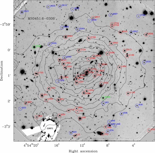
Figure 1. GMOS-N i'-band image of MS0451.6−0305 with contours of the XMM-Newton data overlaid. The field covers approximately 5 5 × 55. Red circles: confirmed cluster members labeled with their ID number; blue circles: non-members with spectroscopy labeled with their ID number; green diamonds: the two blue stars included in each mask to facilitate correction of the spectra for telluric absorption lines. The X-ray image is the sum of the images from the two XMM-Newton EPIC-MOS cameras. The X-ray image has been smoothed such that the structure seen is significant at the 3σ level or higher. The spacing between the contours is logarithmic with a factor of 1.5 between each contour. The GMOS-N on-instrument wavefront sensor used for guiding vignettes the field in the lower left, marked with "OIWFS."
Download figure:
Standard image High-resolution imageThe massive cluster of galaxies RXJ0152.7−1357 was discovered from ROSAT data by three different surveys: the ROSAT Deep Cluster Survey (RDCS) and the Wide Angle ROSAT Pointed Survey (WARPS; see Ebeling et al. 2000), as well as the Bright Serendipitous High-Redshift Archival Cluster (SHARC) survey (Nichol et al. 1999). X-ray observations from XMM-Newton and Chandra (Jones et al. 2004; Maughan et al. 2003) show that the cluster consists of two sub-clumps and support the view that RXJ0152.7−1357 is in the process of merging from two clumps of roughly equal mass. See Jørgensen et al. (2005) for a figure of the XMM-Newton data overlaid on our i'-band imaging data. Demarco et al. (2010) used spectroscopic and photometric data to study the star formation history in RXJ0152.7−1357 and found that the data support a downsizing scenario in which there is a ≈1.5 Gyr age difference between the older high-mass (passive) galaxies (Mass > 1010.9 M☉) and the younger low-mass galaxies (Mass < 1010.4 M☉), and that the low-mass galaxies just in the last 1 Gyr stopped forming stars. For our adopted cosmology, this is equivalent to formation redshifts of zform = 1.6 and 1.1 for the high- and low-mass galaxies, respectively.
RXJ1226.9+3332 is also one of the most X-ray luminous clusters at z > 0.5. The cluster as discovered in the WARPS survey (Ebeling et al. 2001). Figure 2 shows the XMM-Newton data together with our i'-band imaging. The substructures in X-ray surface brightness for RXJ1226.9+3332 are associated with active galactic nuclei (AGNs; see Section 7), and the X-ray structure of the cluster is that of a relaxed structure. However, from the temperature map of the X-ray gas based on XMM-Newton data, Maughan et al. (2007) find evidence for a recent merger event as an off-center sub-clump of X-ray gas that shows higher X-ray temperature and is associated with a local over-density in the galaxy distribution about 45'' to the southwest of the cluster center.
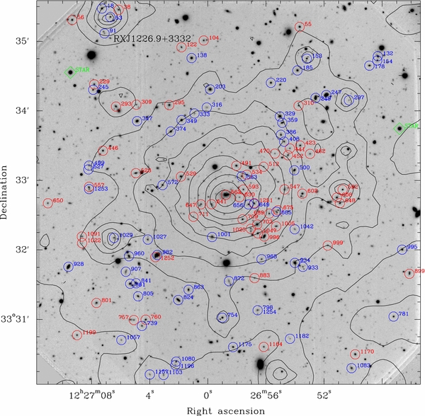
Figure 2. GMOS-N i'-band image of RXJ1226.9+3332 with contours of the XMM-Newton data overlaid. The field covers approximately 55 × 55. Symbols and X-ray contours are the same as in Figure 1. The structure in the X-ray emission seen in the outer part of the cluster can be associated with AGNs, either background (ID 53, 153, 754) or in the cluster (ID 592). The object ID 1029 is a blue point source, possibly also a background AGN, though the spectrum has too low S/N to allow a determination of the redshift.
Download figure:
Standard image High-resolution imageCompared to our chosen low-redshift rich clusters of galaxies, Coma and Perseus, RXJ0152.7−1357 is similar in X-ray luminosity to Perseus, while MS0451.6−0305 and RXJ1226.9+3332 have X-ray luminosities 2–2.5 times that of Perseus. The X-ray luminosity of Coma is significantly lower, being about 55% that of Perseus (see Table 1). As summarized above, substructure is also present to a varying degree in the intermediate-redshift clusters. Thus, while all five clusters are very massive, environmental differences may still play a role in the evolution of their galaxy population.
3. OBSERVATIONAL DATA—GROUND-BASED
Imaging and spectroscopy of the three clusters were obtained for the GCP with the Gemini Multi-Object Spectrograph on Gemini North (GMOS-N). See Hook et al. (2004) for a detailed description of GMOS-N. The instrument information is listed in Table 2, while the Gemini program IDs and observing dates are given in Table 3. The observations are summarized in Tables 4 and 5. The details of the observations of RXJ0152.7−1357 are given in Jørgensen et al. (2005). However, for completeness this cluster is also included in the summary tables in the current paper, with the data reproduced from Jørgensen et al. All programs executed in Director's Discretionary time or in the usual queue were obtained specifically for GCP. These data and the data obtained in engineering time are in the following referred to as the "GCP data."
Table 2. Gemini North Instrumentation
| Parameter | Value |
|---|---|
| Instrument | GMOS-N |
| CCDs | 3 × E2V 2048×4608 |
| r.o.n.a | (3.5,3.3,3.0) e− |
| Gaina | (2.10,2.337,2.30) e−/ADU |
| Pixel scale | 0 0727 pixel−1 0727 pixel−1 |
| Field of view | 55 × 55 |
| Imaging filters | g'r'i'z' |
| Grating | R400_G5305 |
| Spectroscopic filter | OG515_G0306 |
| Wavelength rangeb | 5000–10000Å |
Notes. aValues for the three detectors in the array. bThe exact wavelength range varies from slitlet to slitlet.
Download table as: ASCIITypeset image
Table 3. GMOS-N Observations
| Cluster | Program ID | Dates | Data Type | Program Type |
|---|---|---|---|---|
| (UT) | ||||
| MS0451.6−0305 | GN-2001B-DD-3 | 2001 Dec 25 | Imaging | DDa |
| GN-2002B-Q-29 | 2002 Sep 12 to 2002 Sep 16 | Imaging | Queue | |
| GN-2003B-Q-21 | 2003 Dec 24 | Imaging | Queue | |
| GN-2002B-DD-4 | 2002 Dec 31 to 2003 Jan 2 | Spectroscopy | DD in queue | |
| GN-2003B-DD-3 | 2003 Dec 19 to 2003 Dec 23 | Spectroscopy | DD in queue | |
| RXJ1226.9+3332 | GN-2003A-DD-4 | 2003 Jan 31 to 2003 May 6 | Imaging | DD in queue |
| GN-2003A-SV-80 | 2003 Mar 13 | Imaging | Engineering | |
| GN-2004A-Q-45 | 2004 Feb 17 to UT 2004 Jul 20 | Spectroscopy | Queue | |
| GN-2003A-C-1 | 2003 Apr 29 to 2003 May 1 | Spectroscopy | Classical | |
| GN-2004A-C-8 | 2004 Mar 17 to 2004 Mar 18 | Spectroscopy | Classical |
Note. aDirector's Discretionary time.
Download table as: ASCIITypeset image
Table 4. GMOS-N Imaging Data
| Cluster | Program ID | Filter | Exposure Time | FWHMa | Sky Brightness | Galactic Extinction |
|---|---|---|---|---|---|---|
| ('') | (mag arcsec−2) | (mag) | ||||
| MS0451.6−0305 | GN-2003B-Q-21 | g' | 6 × 600 s | 0.80 | 22.28 | 0.127 |
| GN-2002B-Q-29 | r' | 15 × 600 s (2 frames in twilight) | 0.57 | 20.87 | 0.099 | |
| GN-2001B-DD-3,2B-Q-29 | i' | 6 × 600 s (dark sky) | ||||
| +2 × 300 s (gray sky) | 0.71 | 18.43 | 0.078 | |||
| GN-2001B-DD-3 | z' | 19 × 600 s (bright sky) | 0.72 | 18.52 | 0.064 | |
| RXJ0152.7−1357 | GN-2002B-Q-29,SV-90 | r' | 12 × 600 s | 0.68 | 20.65 | 0.042 |
| i' | 7 × 450 s (dark sky) | 0.56 | 19.63 | 0.033 | ||
| +100 × 120 s (bright sky) | ||||||
| z' | 13 × 450 s (dark sky) | 0.59 | 19.16 | 0.027 | ||
| +14 × 450 s (bright sky) | ||||||
| RXJ1226.9+3332 | GN-2003A-DD-4,SV-80 | r' | 9 × 600 s | 0.75 | 21.30 | 0.056 |
| i' | 7 × 300 s + 3 × 360 s | 0.78 | 20.58 | 0.044 | ||
| z' | 29 × 120 s (gray sky) | 0.68 | 19.90 | 0.036 |
Note. aImage quality measured as the average FWHM of 7–10 stars in the field from the final stacked images.
Download table as: ASCIITypeset image
Table 5. GMOS-N Spectroscopic Data
| Cluster | Program ID | Exposure Time | Nexpa | FWHMb | σinstc | Apertured | Slit Lengths | S/Ne |
|---|---|---|---|---|---|---|---|---|
| ('') | ('') | ('') | ||||||
| MS0451.6−0305 | GN-2002B-DD-4, | |||||||
| GN-2003B-DD-3 | 40,500 s + 32,400 s | 27 | 0.78 | 3.172 Å, 143 km s−1 | 1 × 1.40, 0.68 | 4.1–13.5 | 77 | |
| RXJ0152.7−1357 | GN-2002B-Q-29 | 77,960 s | 25 | 0.65 | 3.065 Å, 116 km s−1 | 1 × 1.15, 0.62 | 5–14 | 31 |
| RXJ1226.9+3332 | GN-2004A-Q-45 | 64,800 s + 64,800 s | 72 | 0.68 | 3.076 Å, 113 km s−1 | 1 × 0.85, 0.53 | 2.75 | 48 |
| RXJ1226.9+3332 | GN-2003A-C-1 | 12,000 s + 12,000 s | 10 | 0.66 | 3.856 Å, 142 km s−1 | 1.25 × 0.85, 0.60 | 2.5–14 | 29 |
| RXJ1226.9+3332 | GN-2004A-C-8 | 7200 s | 4 f | 0.65 | 3.856 Å, 142 km s−1 | 1.25 × 0.85, 0.60 | 2.5–14 | 15 |
Notes.
aNumber of individual exposures.
bImage quality measured as the average FWHM at 8000 Å of either the blue stars included in the masks (GN-2002B-DD-4, GN-2002B-Q-29, GN-2003B-DD-3, GN-2003B-Q-21, and GN-2004A-Q-45) or of the QSOs/AGNs included in the masks (GN-2004A-C-8). For GN-2003A-C-1, the FWHM is measured at 7930 Å from the one QSO included in the mask.
cMedian instrumental resolution derived as σ in Gaussian fits to the skylines of the stacked spectra. The second entry is the equivalent resolution in km s−1 at 4300 Å in the rest frame of the clusters.
dThe first entry is the rectangular extraction aperture (slit width × extraction length). The second entry is the radius in an equivalent circular aperture,  , cf. Jørgensen et al. (1995b).
eMedian S/N per Å in the rest frame of the cluster.
fA fifth exposure was taken but contains no significant signal from the science targets.
, cf. Jørgensen et al. (1995b).
eMedian S/N per Å in the rest frame of the cluster.
fA fifth exposure was taken but contains no significant signal from the science targets.
Download table as: ASCIITypeset image
In addition, we use public spectroscopic data for RXJ1226.9+3332 from programs GN-2003A-C-1 and GN-2004A-C-8 available from the Gemini Science Archive (GSA); see Table 3. These data are referred to as the "GSA data." The imaging data from these programs were not used in the present paper.
The imaging for each cluster covers one GMOS-N field, which is approximately 55 × 55. All spectroscopic observations were obtained using GMOS-N in the multi-object spectroscopic mode. One GMOS mask was used for RXJ0152.7−1357 (Jørgensen et al. 2005), while for MS0451.6−0305 and RXJ1226.9+3332 observations were obtained using two GMOS masks in order to cover more objects, while including the faintest in both masks. The GSA data were obtained with three masks for RXJ1226.9+3332. There is some overlap in spectroscopic targets between the GPC data and the GSA data. We use these targets to ensure consistent calibration of the velocity dispersions and line indices as described in Appendix B.7. However, in the analysis we give our higher S/N GCP data preference over the GSA data for targets in common.
All spectroscopic observations for the GCP used the R400 grating and a slit width of 1'', while the GSA data were obtained with R400 and a slit width of 125. The resulting instrumental resolutions in the rest frames of the clusters are listed in Table 5. For program GN-2004A-Q-45 we used the nod-and-shuffle mode of GMOS-N. All other spectroscopic data were taken in the conventional mode.
For the cluster members, the S/N per Å in the rest frame of the galaxies was derived from the rest-frame wavelength interval 4100–4600 Å for RXJ0152.7−1357 and RXJ1226.9+3332 and 4100–5500 Å for MS0451.6−0305. The median S/N for spectra in each of the clusters is listed in Table 5. The S/N for the individual galaxies in MS0451.6−0305 and RXJ1226.9+3332 is listed in Tables 21 and 23 in Appendix B. The information for RXJ0152.7−1357 can be found in Jørgensen et al. (2005).
3.1. Imaging
The GMOS-N imaging data for MS0451.6−0305 and RXJ1226.9+3332 were reduced and co-added using the same methods as for the RXJ0152.7−1357 imaging data (Jørgensen et al. 2005). One co-added image was produced for each filter and field. The co-added images were then processed with SExtractor v.2.1.6 (Bertin & Arnouts 1996) as described in Jørgensen et al.
The photometry was standard calibrated using the magnitude zero points and color terms derived in Jørgensen (2009). The absolute accuracy of the standard calibration is expected to be 0.035–0.05 mag, as described in that paper. Tables 13 and 14 list the photometry for MS0451.6−0305 and RXJ1226.9+3332 calibrated to the Sloan Digital Sky Survey (SDSS) system. Similar photometry for RXJ0152.7−1357 can be found in Jørgensen et al. (2005). The r'-band imaging for MS0451.6−0305 was obtained in significantly better seeing than the other bands, and therefore is significantly deeper. Object detection was done in the r' band. Due to the difference in seeing the colors involving the r' band are expected to be affected by a systematic error of ≈0.05 mag, with the galaxies being too blue. As this systematic error has no significant effect on our analysis, we have chosen not to correct the colors for the difference in seeing.
The Galactic extinction in the direction of the three clusters is AB = 0.14, 0.064, and 0.085 for MS0451.6−0305, RXJ0152.7−1357, and RXJ1226.9+3332, respectively (Schlegel et al. 1998). Using the effective wavelength of the filters used for the photometry and the calibration from Cardelli et al. (1989) we derive the extinction on those filters; see Table 4. The photometry in Tables 13 and 14 has not been corrected for the Galactic extinction.
We have compared the GMOS-N photometry with available literature data for the fields; details can be found in Appendix A. Based on these comparisons, we conclude that the photometry is calibrated to an external accuracy of 0.05 mag.
3.2. Spectroscopy
The principles of the spectroscopic sample selection for the project are described in Jørgensen et al. (2005). In brief, sample selection is based on the GMOS photometry. Stars and galaxies are separated using the SExtractor classification parameter class_star derived from the image in the i' filter. For the purpose of selecting targets for the spectroscopic observations we choose a threshold of 0.80, i.e., objects with class_star < 0.80 in the i'-image are considered galaxies. In practice, this excludes galaxies with effective radius re ⩽ 015 (re ⩽ 1 kpc). However, it was more important for the planning of our observations that the selected spectroscopic targets had a high probability of being galaxies rather than foreground stars. Then we use the total magnitude in i' and the available colors to define four classes of objects in each field. The aim is to use a color selection that includes likely cluster members. Table 6 summarizes the definition of these four classes for each of the three clusters. The classes are shown in Figures 3 and 4. For RXJ1226.9+3332 the (i' − z') colors are used as the primary color selection, while for MS0451.6−0305 both (r' − z') and (i' − z') colors are used. The classes are used in the selection of the spectroscopic sample as described in Jørgensen et al. (2005). Objects in classes 1 and 2 are likely to be cluster members. For each field, roughly equal numbers of objects from each of these two classes are included. Empty spaces in the mask designs are filled with class 3 objects if possible. This class may include blue cluster members or cluster members too faint to derive all spectroscopic parameters due to the resulting S/N of the spectroscopic observations. Any remaining space in the mask designs is filled with class 4 objects. The brighter and bluer objects in this class are in general not expected to be members of the cluster, while the fainter and redder objects in this class may be faint cluster members. The selection criteria for galaxies included in the analysis are described in Section 8. Here we note that any observed galaxy for which the properties meet the final selection criteria is included in the analysis, independent of its class in this initial selection used for the spectroscopic observations. We have visualized this by marking galaxies included in the analysis with red triangles in Figures 3(a) and 4(a).
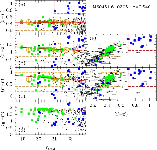
Figure 3. MS0451.6−0305: color–magnitude and color–color diagrams. Only galaxies (class_star < 0.80 in the i' filter) with i' ⩽ 23 mag are shown. The magnitudes are the total magnitudes, while all colors are aperture colors. The photometry has been corrected for the Galactic extinction; see Section 3.1. Green filled boxes: confirmed cluster members in our spectroscopic sample; blue filled boxes: non-members with spectroscopy; small black points: galaxies without spectroscopy. Galaxies included in the analysis are in panel (a) shown with red open triangles overplotted on the green boxes. Red lines: the red sequence. The slope for the color–magnitude relation in (i' − z') is not significantly different from zero. Thus, the line marks the median color. The orange dashed lines and circled numbers show the object classes; see Section 3.2. The orange dashed lines in panels (e) and (f) outline the sample limits in the colors for objects in classes 1 and 2; see Section 3.2. The red dashed lines in panels (a), (e), and (f) outline the sample limits for the background galaxy sample described in Section 3.2.
Download figure:
Standard image High-resolution image
Figure 4. RXJ1226.9+3332: color–magnitude and color–color diagrams. Only galaxies (class_star < 0.80 in the i' filter) with i' ⩽ 23.9 mag are shown. The magnitudes are the total magnitudes, while all colors are aperture colors. The photometry has been corrected for the Galactic extinction; see Section 3.1. Green filled boxes: confirmed cluster members in our spectroscopic sample; blue filled boxes: non-members with spectroscopy; green open boxes: confirmed cluster members from the GSA data; blue open boxes: non-members with spectroscopy from the GSA data; small black points: galaxies without spectroscopy. Galaxies included in the analysis are in panel (a) shown with red open triangles overplotted on the green boxes. Red lines: the median colors for the red sequence. The slopes for the color–magnitude relations are not significantly different from zero. The orange dashed lines and circled numbers show the object classes; see Section 3.2. The orange dashed lines in panels (d) and (e) outline the sample limits in the colors for objects in classes 1 and 2; see Section 3.2.
Download figure:
Standard image High-resolution imageTable 6. Selection Criteria for Spectroscopic Samples
| Cluster | Object Class | Selection Criteria |
|---|---|---|
| MS0451.6−0305a | 1 | 18 ⩽ i' ⩽ 20.7∧0.3 ⩽ (i' − z') ⩽ 0.6∧0.7 ⩽ (r' − z') ⩽ 1.6 |
| 2 | 20.7 < i' ⩽ 21.4∧0.3 ⩽ (i' − z') ⩽ 0.6∧0.7 ⩽ (r' − z') ⩽ 1.6 | |
| 3 | (18.0 ⩽ i' ⩽ 21.4∧0.2 ⩽ (i' − z') < 0.3∧0.4 ⩽ (r' − z') < 0.7)∨ | |
| (21.4 ⩽ i' ⩽ 22.2∧0.2 ⩽ (i' − z') ⩽ 0.6∧0.4 ⩽ (r' − z') ⩽ 1.6) | ||
| 4 | (18.0 ⩽ i' ⩽ 22.2∧(i' − z') < 0.2)∨(22.2 < i' ⩽ 22.5∧(i' − z') < 0.6) | |
| RXJ0152.7−1357b | 1 | 20.35 ⩽ i' ⩽ 21.35∧(i' − z') ⩾ 0.7 |
| 2 | 21.35 < i' ⩽ 22.35∧(i' − z') ⩾ 0.7 | |
| 3 | 20.35 ⩽ i' ⩽ 22.35∧0.45 ⩽ (i' − z') < 0.7 | |
| 4 | (i' < 20.35∧0.45 ⩽ (i' − z') < 0.7)∨(i' > 22.35∧(i' − z') ⩾ 0.7) | |
| RXJ1226.9+3332 | 1 | 19.5 ⩽ i' ⩽ 21.9∧0.6 ⩽ (i' − z') ⩽ 0.8∧1.0 ⩽ (r' − i') ⩽ 1.4 |
| 2 | 21.9 < i' ⩽ 22.6∧0.6 ⩽ (i' − z') ⩽ 0.8∧1.0 ⩽ (r' − i') ⩽ 1.4 | |
| 3 | (21.9 ⩽ i' ⩽ 22.6∧0.275 ⩽ (i' − z') ⩽ 0.6)∨ | |
| (22.6 ⩽ i' ⩽ 23.0∧0.275 ⩽ (i' − z') ⩽ 0.8) | ||
| 4 | (19.5 ⩽ i' ⩽ 21.9∧(i' − z') < 0.6)∨(21.9 < i' ⩽ 23.0∧(i' − z') < 0.275)∨ | |
| (23.0 < i' ⩽ 23.8∧(i' − z') ⩽ 0.8) |
Notes. aAt the time of the sample selection for MS0451.6−0305 only r', i', and z' imaging were available. bSelection criteria for RXJ0152.7−1357 reproduced from Jørgensen et al. (2005).
Download table as: ASCIITypeset image
Redshift data for MS0451.6−0305 from the CNOC survey (Ellingson et al. 1998) were used to optimize inclusion of cluster members. In the mask design galaxies that are known cluster members based on these data were given preference over galaxies without redshift information. Known non-members were assigned to class 4 and only included in the mask if no object from the other classes could be used to fill the available space.
The masks for MS0451.6−0305 also include 12 objects selected to have (i' − z') ⩾ 0.7 and (r' − z') ⩾ 1.1 and therefore be candidate background galaxies with redshifts larger than about 0.75 and passive stellar populations. These are enclosed by the red box in Figures 3(a), (e), and (f), and are not discussed further in this paper though we do derive and list their redshifts.
The sample selection for the GSA data used for RXJ1226.9+3332 is not known. We note that in addition to cluster members on the red sequence, the data contain a number of bluer member and non-member galaxies, as well as some AGNs.
The spectroscopic samples are marked in Figures 1 and 2. For each mask in the GCP observations, two blue stars were included in order to obtain a good correction for the telluric absorption lines. The blue stars are also marked in figures.
The MS0451.6−0305 spectroscopic data were reduced in the same way as done for the RXJ0152.7−1357 data (Jørgensen et al. 2005). The only difference was that we applied our established correction for the charge diffusion in the red as described in Appendix B. The correction slightly improves the sky subtraction for these short slits.
The RXJ1226.9+3332 GSA data were reduced in a similar way, with the exception that for some of the very short slitlets with the objects very close to the end of the slitlet, sky subtraction was possible only after the wavelength calibration had been applied. This in general leads to poorer sky subtraction as the (strong) skylines are being interpolated onto the rectified wavelength scale before the sky signal is subtracted out.
The RXJ1226.9+3332 GCP data were obtained using GMOS-N in the nod-and-shuffle mode (Glazebrook & Bland-Hawthorn 2001). The reduction of these data involved construction of special flat fields that take into account the shuffling of the data on the detector array, as well as a correction for the effect of charge diffusion in the far-red wavelength region.
The details of the reductions of all the spectroscopic data are described in Appendix B. The final data products are cleaned and averaged spectra that have been wavelength calibrated and calibrated to a relative flux scale. Both the extracted one-dimensional (1D) and the 2D spectra are kept after the basic reductions. However, in this paper we use only the 1D spectra.
The co-added 1D spectra were used for deriving the redshifts, velocity dispersions, absorption line indices, and emission line equivalent widths of the galaxies. The details are described in Jørgensen et al. (2005) and in Appendix B. In the following analysis we use the Lick/IDS absorption line indices for CN2, Fe4383, C4668, Mgb, Fe5270, and Fe5335 (Worthey et al. 1994). We use HβG (see González 1993; Jørgensen 1997) in place of the Lick/IDS definition for Hβ. We also use the higher order Balmer line indices HδA and HγA (Worthey & Ottaviani 1997) and the CN3883 index defined by Davidge & Clark (1994). The uncertainties on the line indices were estimated both from the local S/N of the spectra and from internal comparisons of indices derived from stacking subsets of the frames available for each cluster. In the following we use the uncertainties from the latter method as these are larger than uncertainties based on the S/N. Table 19 in Appendix B summarizes the uncertainties.
For galaxies with detectable emission from [O ii] we determined the equivalent width of the [O ii]λλ3726,3729 doublet, in the following referred to as the "[O ii] line."
Tables 22 and 24 in Appendix B list the derived line indices and the measurements of the [O ii] equivalent widths for members of MS0451.6−0305 and RXJ1226.9+3336. The data for RXJ0152.7−1357 are available in Jørgensen et al. (2005).
In the analysis involving the two higher order Balmer line indices HδA and HγA, we use the combined index as defined by Kuntschner (2000) (HδA + HγA)' ≡ −2.5log (1 − (HδA + HγA)/(43.75 + 38.75)). For the iron indices in the visible region, we use the average iron index 〈Fe〉 ≡ (Fe5270 + Fe5335)/2 rather than the individual indices.
4. OBSERVATIONAL DATA—HST
The three clusters have publicly available data obtained with HST/ACS. Table 7 summarizes the data used in this paper. A large mosaic of fields was observed for MS0451.6−0305. However, we only use the data that cover our spectroscopic sample.
Table 7. HST/ACS Imaging Data
| Cluster | No. of Fields | Filter | Total texp | Program ID |
|---|---|---|---|---|
| (s) | ||||
| MS0451.6−0305 | 6 | F814W | 4072 | 9836 |
| RXJ0152.7−1357 | 4 | F775W | 4800 | 9290 |
| RXJ1226.9+3332 | 4 | F814W | 4000 | 9033 |
Download table as: ASCIITypeset image
For RXJ0152.7−1357 and RXJ1226.9+3332, we use the photometric parameters derived as part of the project and published in Chiboucas et al. (2009). The data for MS0451.6−0305 were processed in the same way. Specifically, we stacked the images using the drizzle technique (Fruchter & Hook 2002) and derived effective radii, magnitudes, and surface brightnesses using the fitting program GALFIT (Peng et al. 2002). Table 15 in Appendix A lists the derived parameters for the spectroscopic sample. We have compared the derived parameters with data from S. Moran (2011, private communication) and find our photometry to be consistent with that of Moran to within 0.04 mag; see Appendix A for details.
The HST photometry was transformed to the SDSS i' as described in Appendix A. Then the photometry was calibrated to rest-frame B band, using the colors of the galaxies determined from the GMOS-N photometry. The calibration was established using stellar population models from Bruzual & Charlot (2003) as described in Jørgensen et al. (2005). The calibrations at the cluster redshifts of all three clusters are listed in Appendix A, Table 18.
5. LOW-REDSHIFT COMPARISON DATA
As in Jørgensen et al. (2005), we use our data for galaxies in Coma, Perseus, and A194 as the low-redshift comparison sample. The line indices and velocity dispersions for the Coma cluster galaxies are published in Jørgensen (1999). We use the same B-band photometry for the cluster as in Jørgensen et al. (2005). The spectroscopic data for Perseus and A194 are the same as used in Jørgensen et al. (2005). Table 8 summarizes the number of galaxies in each of the cluster with available velocity dispersions and line indices. The Coma cluster data do not include line indices blueward of 4700 Å. The sample selection for the Coma cluster sample is detailed in Jørgensen (1999). The Perseus and A194 samples were selected in a similar fashion. Briefly, the initial selection was based on morphological classifications, excluding spiral and irregular galaxies. Apparent magnitude limits were applied, which with our adopted cosmology are equivalent to an absolute magnitude limit of MB = −18.6 mag for all the low-redshift clusters. The Coma cluster sample is 93% complete to this limit. The Perseus and A194 samples span the full magnitude range from the brightest cluster galaxy to MB = −18.6 mag but are not intended to be complete. Galaxies with emission lines or with Mass < 1010.3 M☉ were excluded from the analysis. Despite initially being selected morphologically, the resulting samples are equivalent to a color selection, followed by exclusion of spirals, irregulars, emission line galaxies, and low-mass galaxies. Thus, the selection criteria match those used for the selection of the intermediate-redshift galaxies included in the analysis; see Section 8.
Table 8. Low-redshift Comparison Data
| Cluster | Redshift | N(log σ) | N(blue) | N(HβG) | N(Mgb,〈Fe〉) |
|---|---|---|---|---|---|
| Perseus | 0.018 | 63 | 51 | 58 | 63 |
| A0194 | 0.018 | 17 | 14 | 10 | 10 |
| Coma | 0.024 | 116 | ... | 90 | 68a |
Notes. N(log σ): number of galaxies with velocity dispersion measurements; N(blue): number of galaxies with measurements of line indices blueward of 4700 Å; N(HβG): number of galaxies with measurement of HβG; N(Mgb, 〈Fe〉): number of galaxies with measurement of Mgb and 〈Fe〉. a115 galaxies in Coma have measurements of Mg2.
Download table as: ASCIITypeset image
The Coma cluster galaxies have Mg2 on the Lick/IDS system measured for all galaxies with measured velocity dispersion, but Mgb only for those with original data from Jørgensen (1999). The older literature data, which were calibrated to consistency in that paper, did not include published Mgb measurements. Due to the very broad continuum bands for Mg2 consistent calibration of this index to the Lick/IDS system relies on sufficient duplicate observations of galaxies or stars for which Mg2 is already calibrated. Further, we have no access to the spectra on which the literature data for Mg2 are based. It is therefore not an option to remeasure Mg2 in a system that relies on flux-calibrated spectra rather than in the Lick/IDS system. To take advantage of the old Lick/IDS Mg2 measurements, we therefore choose to calibrate them to Mgb, which has narrower passbands and can reliably be calibrated from spectra on a relative flux scale. The disadvantage is the slightly higher relative uncertainty on Mgb compared to that of Mg2. For those galaxies in the Coma sample without Mgb, we transform Mg2 to Mgb using the relation

established from the 68 galaxies in the Coma sample (Jørgensen 1999) for which both indices are available. The rms scatter of the relation is 0.033, all of which can be explained by the measurement uncertainties on the two indices. Thus, the relation has no significant intrinsic scatter.
6. MODELS
6.1. Single Stellar Population Models
In the analysis of the line index strengths we use the SSP models from Thomas et al. (2011) for a Salpeter (1955) initial mass function (IMF). These authors model the Lick/IDS indices on a flux-calibrated system, which makes them ideal for comparison with our data. They also provide models for different abundance ratios. We use their base models for different values of [α/Fe], where the α-elements should be understood as including the carbon, nitrogen, and sodium. Further, we use the carbon and nitrogen enhanced models. We downloaded the model tables from the Web site provided by D. Thomas (http://www.icg.port.ac.uk/~thomasd).
The models do not provide predictions for the M/L ratios and CN3883. Maraston (2005) modeled the M/L ratios for solar abundance ratios and otherwise used the same model ingredients as Thomas et al. The dependency of the M/L ratios on varying abundance ratios (at fixed metallicity) are in general poorly understood and often assumed to be insignificant as done by Maraston. In our discussion we also investigate the effect of differences in the IMF slope. To do so, we use the models from Vazdekis et al. (2010), but note that these models cover solar abundance ratios only.
The strong index CN3883 is not yet modeled by any of the commonly used stellar population models, which also vary the abundance ratios. Rather than use the weaker indices CN1 and CN2 we instead estimate how CN3883 depends on age, metallicity, and abundance ratios using two approaches. First, we use the model spectra used by Maraston & Strömbäck (2011) to derive CN3883 and CN2. The models are based on the same ingredients as the models from Thomas et al. (2011), but cover only solar [α/Fe]. Second, we determine an empirical relation between CN3883 and CN2 and then transform the stellar population model values for CN2 to the equivalent CN3883. CN1 and CN2 probe the same features in the spectra. However, CN2 excludes Hδ in its blue continuum passband and is therefore preferred over CN1 (Worthey et al. 1994).
Figure 5 shows CN3883 versus CN2 and the best-fit relation

with an rms scatter of 0.041. The residuals were minimized in CN3883 as the goal is to predict CN3883 based on the CN2 values. The relation has an intrinsic scatter of about 0.03 in CN3883. This relation has not previously been established in the literature. As the passbands for CN3883 contain some higher order Balmer lines, one might expect that (part of) the intrinsic scatter of the relation is due to differences in the strengths of the Balmer lines. However, we found no dependence of the residuals on the Balmer line index (HδA + HγA)'. Similarly including (HδA + HγA)' as a parameter in the fit does not lower the scatter of the established relation. For the redshifts of RXJ0152.7−1357 and RXJ1226.9+3332, the passband for CN2 coincides with the strong telluric absorption around 760–770 nm. However, CN2 is only used to establish Equation (4) and not in the analysis itself. Excluding RXJ0152.7−1357 and RXJ1226.9+3332 from the fit results in slightly steeper relation with a slope of 1.00 ± 0.13. This relation is also shown in Figure 5. None of the results in our analysis change significantly if we were to adopt this steeper slope. Thus, we adopt Equation (4) as the best fit. Figure 5 also shows the model values based on Maraston & Strömbäck (2011). These implicate stronger CN3883 at CN2 > 0.08 than found from the data. It is beyond the scope of this paper to investigate the reason for this. However, we note that CN3883 derived from the Maraston & Strömbäck model spectra would indicate roughly a factor of two stronger dependency on age and metallicity than if instead we use the transformation in Equation (4). However, because the values from the Maraston & Strömbäck model spectra do not reproduce our data, we choose to use Equation (4) to transform the model values for CN2 (from Thomas et al. 2011) to CN3883, and through that transformation achieve estimates of how CN3883 depends on age, metallicity, and [α/Fe].
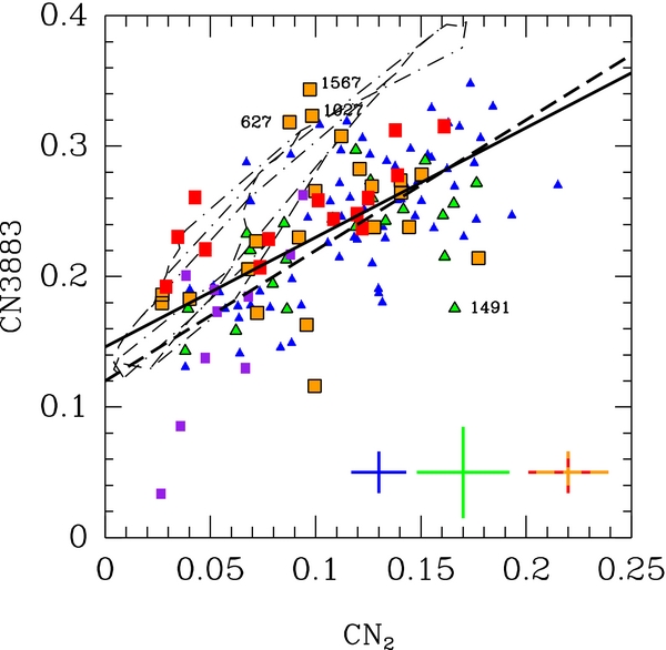
Figure 5. CN3883 vs. CN2 for galaxies without significant emission. Blue triangles: low-redshift sample; green triangles: MS0451.6−0305; orange boxes: RXJ0152.7−1357; red boxes: RXJ1226.9+3332; purple boxes: non-members in the fields of MS0451.6−0305, RXJ0152.7−1357, and RXJ1226.9+3332. Typical uncertainties are shown; see Table 19 in Appendix B. We adopt the same uncertainties for RXJ0152.7−1357 as for RXJ1226.9+3332. Black solid line: best-fit relation, Equation (4). Black dashed line: best fit if excluding RXJ0152.7−1357 and RXJ1226.9+3332 members from the fit; see the text. Dot-dashed lines: model predictions based on model spectra from Maraston & Strömbäck (2011); see the text for discussion. The four labeled galaxies were omitted from the fit, as the indices may be affected by systematic residuals from the sky subtraction. The relation shown as the solid line is used to transform model predictions for CN2 to CN3883.
Download figure:
Standard image High-resolution imageTo enable studying the metallicity independent of the [α/Fe] abundance ratios, we use the combined magnesium–iron index [MgFe] ≡ (Mgb × 〈Fe〉)1/2 first used by González (1993). The models predict this index to be independent of the [α/Fe] abundance ratios. Similarly we experimented to find a combination of C4668 and Fe4383, which the models also predict to be independent of [α/Fe]. The combined index

has this property, as fitting this index as a function of age, metallicity, and [α/Fe] shows in an insignificant dependence on [α/Fe]. This combined index makes it possible for us to carry out similarly [α/Fe] independent analysis of the higher redshift clusters as is possible at lower redshift using [MgFe]. We have also tested a similarly defined index using CN3883 in place of C4668,

Under the assumption that the transformation from CN2 to CN3883 is valid (Equation (4)), then fitting this index as a function of age, metallicity, and [α/Fe] also results in an insignificant dependence on [α/Fe]. While this index is independent of [α/Fe], its metallicity dependency relative to its age dependency is only about a factor of 1.5, while for [C4668 Fe4383] the same ratio is about 2.8. Thus, the models are better separated in age and metallicity in the [C4668 Fe4383] versus (HδA + HγA)' diagram than when using [CN3883 Fe4383] versus (HδA + HγA)'.
Because our data for the clusters RXJ0152.7−0152 and RXJ1226.9+3332 do not include line indices in the visible (HβG, Mgb, and 〈Fe〉), we have evaluated to what extent line indices in the blue can be used to trace the same properties of the stellar populations as traced by the indices in the visible wavelength region. Figure 6 shows the best choices in the blue versus the line indices in the visible. The higher order Balmer lines and HβG are expected to be closely correlated (Figure 6(a)). However, the data show galaxies with weaker HβG than expected from their (HδA + HγA)' indices. While this may be due to HβG being partly filled in by (very) weak emission, we choose to still include these galaxies in the analysis as the strength of their [O ii] emission meets the sample selection criteria; see Section 8.
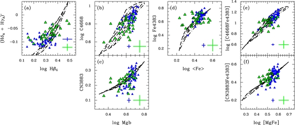
Figure 6. Line indices in the visual vs. the possible equivalents in the blue wavelength region. Blue triangles: low-redshift sample; green triangles: MS0451.6−0305. Stellar population models from Thomas et al. (2011) for [α/Fe] = 0.3 are overlaid. Typical uncertainties are shown in each panel. As not all galaxies have all indices measured, it may be noticed that some galaxies are seemingly missing from some panels.
Download figure:
Standard image High-resolution imageC4668 and CN3883 versus Mgb both approximately follow the locations predicted by the stellar populations' models for [α/Fe] = 0.3 (Figures 6(b) and (c)) and we therefore consider them both as viable candidates for use in the blue in place of Mgb. However, it is important to note that the models assume that the carbon and nitrogen abundance ratios, [C/Fe] and [N/Fe], follow the [α/Fe] abundance ratio. As C4668 and CN3883 both depend on the carbon and nitrogen abundances, the two indices trace [C/Fe] and [N/Fe], which are then assumed to be the same as [α/Fe]. We return to the question of additional enhancement of carbon or nitrogen in Section 10. The two iron indices 〈Fe〉 and Fe4383 are expected to be closely correlated, see Figure 6(d). The low-redshift data are in agreement with this prediction, while the MS0451.6−0305 sample show a larger scatter relative to the predicted relation between 〈Fe〉 and Fe4383. This can be explained by the larger uncertainties on the iron indices for MS0451.6−0305. The indices [C4668 Fe4383] and [CN3883 Fe4383] trace metallicity as well as [MgFe]; see Figures 6(e) and (f).
In our analysis, we will use the models to identify general trends of the indices with varying ages, metallicities, and abundance ratios. To make this more straightforward we fit the model index values as a function of age, total metallicity [M/H] and abundance ratio [α/Fe]. All fits to the models are established for ages between 2 and 15 Gyr, [M/H] from −0.33 to 0.67, and [α/Fe] from −0.3 to 0.5. The fits were established as least-squares fits with the residuals minimized in the line indices. The model fits are listed in Table 9. In addition, we use the carbon and nitrogen enhanced models to establish the dependence of the indices C4668 and CN3883 on [C/α] and [N/α]. The dependence of carbon and nitrogen enhancements is decoupled from the dependence on age, metallicity, and [α/Fe] as inclusion of [C/α] and [N/α] in the fits changes the other coefficients with negligible amounts. The other indices used in our analysis depend only very weakly on [C/α] and [N/α] (Thomas et al. 2011).
Table 9. Predictions from Single Stellar Population Models
| Relation | rms | Reference | |
|---|---|---|---|
| (1) | (2) | (3) | |
| log M/LB | =0.935log age + 0.337[M/H] − 0.053 | 0.022 | Maraston (2005) |
| (HδA + HγA)' | =−0.126log age − 0.106[M/H] + 0.091[α/Fe] + 0.017 a | 0.011 | Thomas et al. |
| log HβG | =−0.230log age − 0.108[M/H] + 0.053[α/Fe] + 0.519 | 0.014 | Thomas et al. |
| CN3883 | =0.076log age + 0.150[M/H] + 0.072[α/Fe] + 0.132 | 0.010 | Thomas et al. + Equation (4) |
| CN3883 | =0.084log age + 0.175[M/H] + 0.071[α/Fe] + 0.177[C/α] + 0.117[N/α] + 0.123 | 0.015 | Thomas et al. + Equation (4) |
| log Fe4383 | =0.272log age + 0.331[M/H] − 0.356[α/Fe] + 0.400 | 0.030 | Thomas et al. |
| log C4668 | =0.121log age + 0.484[M/H] + 0.116[α/Fe] + 0.581 | 0.030 | Thomas et al. |
| log C4668 | =0.108log age + 0.475[M/H] + 0.100[α/Fe] + 0.764[C/α] − 0.072[N/α] + 0.596 | 0.031 | Thomas et al. |
| log [C4668 Fe4383] | =0.212log age + 0.594[M/H] + 0.715 b | 0.037 | Thomas et al. |
| log Mgb | =0.242log age + 0.322[M/H] + 0.242[α/Fe] + 0.262 | 0.021 | Thomas et al. |
| log 〈Fe〉 | =0.122log age + 0.260[M/H] − 0.243[α/Fe] + 0.336 c | 0.009 | Thomas et al. |
| log [MgFe] | =0.182log age + 0.292[M/H] + 0.299 d | 0.012 | Thomas et al. |
Notes. Column 1: relation established from the published model values. [M/H] ≡ log Z/Z☉ is the total metallicity relative to solar. [α/Fe] is the abundance of the α-elements relative to iron, and relative to the solar abundance ratio. The age is in Gyr. The M/L ratios are stellar M/L ratios in solar units. Column 2: scatter of the model values relative to the relation. Column 3: reference for the model values. a(HδA + HγA)' ≡ −2.5log (1 − (HδA + HγA)/(43.75 + 38.75)); Kuntschner 2000. b[C4668 Fe4383] ≡ C4668 × (Fe4383)1/3; see Section 6. c〈Fe〉 ≡ (Fe5270 + Fe5335)/2. d[MgFe] ≡ (Mgb × 〈Fe〉)1/2; González 1993.
Download table as: ASCIITypeset image
In the analysis we also use the models to estimate ages, metallicities [M/H], and abundance ratios [α/Fe]. We use HβG versus [MgFe] and (HδA + HγA)' versus [C4668 Fe4383] to estimate ages and [M/H]. The abundance ratios [α/Fe] are derived from Mgb versus 〈Fe〉 and from CN3883 versus Fe4383. As the indices in the visible and the blue do not depend on age, [M/H], and [α/Fe] in identical ways, and the models do not perfectly model the galaxies, we expect that there will be differences between the parameters derived from the visible indices and those based on the blue indices. For example, since CN3883 in some of the galaxies appears to be weaker than expected from the Mgb measurements, given the model predictions (see Figure 6(c)), estimating [α/Fe] from CN3883 versus Fe4383 may result in lower values than when using Mgb versus 〈Fe〉. Further, the metal dependence relative to the age dependence is stronger for [C4668 Fe4383] than for [MgFe] (see Table 9), which in turn may lead to differences in both age and [M/H] estimates. However, we do not mix the parameters derived from the visible indices with those derived from the blue indices, and to a large extent we limit the analysis to using the differences between the clusters for the various parameters. Thus, these issues do not significantly affect our conclusions.
While other stellar population models are available in the literature (e.g., Vazdekis et al. 2010; Schiavon 2007), the models from Thomas et al. are widely used in the field and are readily available for fixed total metallicities, different [α/Fe] abundance ratios, and for carbon or nitrogen enhanced above the [α/Fe] abundance ratio. We tested if it would make a difference for our results if we had used the models from Schiavon (2007). We used models that treat the individual elements the same as done in the base models by Thomas et al., specifically models for which carbon, nitrogen, and sodium abundances follow [α/Fe]. For each model point, total metallicities [M/H] were derived as [M/H] = [Fe/H] + X, where X = −0.18, 0.0, 0.28, and 0.47 for the four model sets of [α/Fe] = -0.2, 0.0, 0.3, and 0.5, respectively (R. Schiavon 2012, private communication). We then fit the model index values as a function of age, [M/H], and [α/Fe] omitting the very low [M/H] and very young age models, as done for the models from Thomas et al. (2011). In general, the fits are very similar to those derived for the models from Thomas et al. with coefficients being within 10% of those listed in Table 9. Relative to the models from Thomas et al., the exceptions are as follows. (1) Mgb and 〈Fe〉 have a weaker dependence on [α/Fe] in the models from Schiavon, while Fe4383 has a stronger [α/Fe] dependence. This affects the exact location of the models in the Mgb–〈Fe〉 and CN3883–Fe4383 diagrams. However, it does not affect our results regarding [α/Fe] variations between clusters or as a function of redshift. (2) CN3883 and C4668 have a weaker dependence on [M/H] in the models from Schiavon. This would result in any measured differences in [M/H] being derived larger if we used the models from Schiavon, but it does not affect our results regarding variations between clusters or as a function of redshift. It should also be noted that the models from Schiavon reach [M/H] >0.2 only for [α/Fe] above solar and that the models do not cover the very strong C4668 indices seen for the most massive galaxies in our samples. Thus, the differences in the resulting fits may, at least in part, be caused by differences in the parameter space covered by the two sets of models.
6.2. Passive Evolution Model
Models for passive evolution assume that the galaxies after an initial period of star formation usually at high redshift, evolve passively without any additional star formation. The models are usually parameterized by a formation redshift zform, which corresponds to the approximate epoch of the last major star formation episode. As the stellar populations in the observed galaxies are assumed to age passively and no other changes take place, the difference between the luminosity weighted mean ages of the stellar populations in the galaxies in each cluster and similar galaxies at the present is expected to be equal to the look-back time for that redshift. For reference, the look-back time for z = 0.89 is 7.3 Gyr with our adopted cosmology.
Thomas et al. (2005) used the properties of nearby early-type galaxies to estimate the formation redshift zform as a function of galaxy velocity dispersion, and through an empirical relation between stellar mass and velocity dispersion as a function of stellar mass. We adopt their model for the high-density cluster environment as our base model for passive evolution and show the model predictions throughout the paper together with our data. As our relation between dynamical mass and velocity dispersion is slightly different from the stellar mass–velocity dispersion relation used by Thomas et al., we adopt our transformation in order to show the model predictions as a function of dynamical mass. For the typical low and high velocity dispersion galaxies (log σ = 2.1 and 2.35) in our sample the model from Thomas et al. implies zform ≈ 1.4 and 2.2, respectively.
A more recent analysis by Thomas et al. (2010) used data from the SDSS to establish the formation redshift as a function of galaxy velocity dispersion and mass, covering primarily lower density environments. Using this model in place of that from Thomas et al. (2005) does not affect our results significantly. Thus, we choose to use the original high-density environment model from Thomas et al. (2005).
In our analysis, we implicitly assume that the galaxies we observe at high redshift are the progenitors to the galaxies in the low-redshift comparison sample. This may not be the case, as discussed in detail by van Dokkum & Franx (2001). We return to this issue in the discussion in Section 12.3.
7. CLUSTER REDSHIFTS, VELOCITY DISPERSIONS, AND SUBSTRUCTURE
Cluster mass, local density, and substructure are key elements of the cluster environment experienced by the galaxies. To the extent that galaxy formation and evolution depend on the cluster environment, we seek to minimize differences caused by the cluster environment in our samples, such that we can compare samples in different clusters under the assumption that they have experienced similar cluster environments. The clusters were therefore selected based on X-ray luminosity. In this section we determine the cluster redshifts and establish cluster membership. We determine the cluster velocity dispersions, σcluster, test for the presence of substructure in the kinematics of the clusters, and evaluate whether the clusters follow common relations between σcluster and the X-ray properties.
The cluster redshifts and velocity dispersions were determined using the bi-weight method described by Beers et al. (1990). Figure 7 shows the distributions of the radial velocities of the three spectroscopic samples. Figures 7(b) and (e) are identical to the information shown in Jørgensen et al. (2005) and are included here for completeness. Table 1 summarizes the redshifts and cluster velocity dispersions. We note that the cluster velocity dispersion of 1450+105−159 km s−1 for MS0451.6−0305 is higher than found by the Borgani et al. (1999) for the CNOC data, who found 1330+111−94 km s−1. The difference is due to the three galaxies with largest |v||| that we include as cluster members as we iteratively include galaxies as cluster members if |v||| < 3σcluster. The three galaxies are ID = 1931, 2127, and 2945. Their inclusion as cluster members does not significantly affect the results found for the scaling relations and stellar populations described in the following sections. If we exclude these three galaxies, then we find σcluster = 1262+81−103 km s−1. Moran et al. (2007a) obtained spectra for a large number of galaxies in MS0451.6−0305. Using data for the galaxies they consider members and the method from Beers et al. we find σcluster = 1363 ± 51 km s−1, confirming the high velocity dispersion of this cluster.

Figure 7. (a)–(c) Redshift distribution of the spectroscopic samples in the three fields. (d)–(f) Distribution of the radial velocities (in the rest frame of the cluster) relative to the cluster redshifts for cluster members, v|| = c(z − zcluster)/(1 + zcluster). None of the radial velocity distributions for the members are significantly different from Gaussian distributions.
Download figure:
Standard image High-resolution imageAs first found by Maughan et al. (2003) based on the X-ray data RXJ0152.7−1357 consists of two sub-clusters; see Jørgensen et al. (2005) for the X-ray data overlaid on our GMOS-N imaging data. The substructure is not reflected in the distribution of the radial velocities, which is consistent with being Gaussian (Jørgensen et al. 2005). This may be due to the relative orientation of the two sub-clusters. We have tested whether the velocity distributions for the two other clusters deviate from Gaussian distributions. We used a Kolmogorov–Smirnov test for this and find probabilities that the samples are drawn from Gaussian distributions of 88% and 98% for MS0451.6−0305 and RXJ1226.9+3332, respectively. Thus, no substructure is detectable in these distributions. MS0451.6−0305 and RXJ1226.9+3332 also do not show any substructure in the X-ray data; see Figures 1 and 2, respectively. The structure seen in the outskirts of RXJ1226.9+3332 can all be associated with AGNs. However, as noted in Section 2 there is other evidence of more subtle substructure in these two clusters.
In Figures 8(a) and (b), we show the cluster velocity dispersions versus the X-ray properties (see Table 1 for the data). The clusters follow the relation between X-ray luminosity and σcluster established by Mahdavi & Geller (2001). They also follow the expected relation between X-ray masses, radii, and σcluster. Thus, the clusters' dynamical properties match their X-ray properties.

Figure 8. Cluster velocity dispersion vs. X-ray properties of the clusters. Triangles: Coma and Perseus; squares: intermediate-redshift clusters. (a) The relation shows L500∝σ4.4cluster at the median zero point of the clusters. The slope is from Mahdavi & Geller (2001). (b) The relation shows the expected slope M500 R−1500∝σ2cluster at the median zero point of the clusters. (c) The cluster mass M500 vs. the redshift. Circles: RXJ0152.7−1357 treated as two clusters. Solid line: example model of cluster mass evolution based on numerical simulations from van den Bosch (2002). Dashed lines: expected scatter in the cluster mass evolution based on Wechsler et al. (2002).
Download figure:
Standard image High-resolution imageThe three intermediate-redshift clusters, Coma, and Perseus are all very massive. However, as cluster masses are expected to grow over time (e.g., van den Bosch 2002), one may question if the intermediate-redshift clusters are viable progenitors for Perseus and Coma. Figure 8(c) shows the cluster mass M500 versus redshift for all the clusters. The solid line shows a typical model of cluster mass evolution based on numerical simulations by van den Bosch (2002) with the dashed lines showing the expected scatter in cluster evolution (e.g., Wechsler et al. 2002). A cluster like the Perseus cluster may originate from a cluster at z = 0.8 that has M500 between 1014 M☉ and 1014.4 M☉. Treating RXJ0152.7−1357 as two clusters (circles in Figure 8(c)) brings the mass of each of the components into this range, though of course the interaction between the two sub-clusters is likely to affect the galaxy evolution (e.g., Jørgensen et al. 2005). RXJ1226.9+3332 and MS0451.6−0305 are both too massive to be viable progenitors for Coma and Perseus, while RXJ1226.9+3332 may be a viable progenitor for MS0451.6−0305. However, it remains to be seen if this also means that their galaxy populations cannot be progenitors of those in Perseus and Coma. Case in point, studies of nearby clusters by Smith et al. (2006) indicate that the local environment, rather than the total mass of clusters, may be the determining factor for the stellar populations in early-type galaxies. As Smith et al. find that the properties of stellar populations depend on the cluster center distance of the galaxy, Rcl, normalized to the size of the cluster, we next investigate if our samples span similar ranges in Rcl R−1500. Figure 9 shows the distributions for the galaxies included in the analysis; see Section 8. From this figure we conclude that the samples in Coma, Perseus, and MS0451.6−0305 have similar distributions in Rcl R−1500. The A194 sample has a few galaxies at Rcl R−1500 > 1, the inclusion of which do not significantly change the relations and distributions established for the low-redshift sample in the following analysis. The samples in RXJ1226.9+3332 and RXJ0152.7−1357 contain a significant number of galaxies at Rcl R−1500 > 1. In the analysis we comment on the properties of these galaxies relative to those closer to the cluster centers.
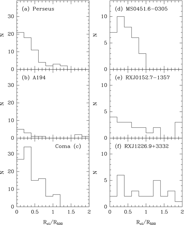
Figure 9. Distribution of cluster center distances Rcl for the galaxies included in the analysis. The distances have been normalized with the cluster size, R500. RXJ0152.7−1357 is treated as two clusters and Rcl determined relative to the nearest of the centers of the two sub-clusters.
Download figure:
Standard image High-resolution image8. THE METHODS AND THE FINAL GALAXY SAMPLE
We characterize the stellar populations in the three clusters galaxies by (1) establishing the FP and other scaling relations and (2) comparing the line index measurements with SSP models and deriving the distributions of the ages, metallicities [M/H], and abundance ratios [α/Fe] determined from the line indices using the SSP models. We use the effective radii and surface brightnesses derived from the fits with r1/4 profiles since the low-redshift comparison sample was fit with r1/4 profiles. However, none of the results depend significantly on this choice.
The fitting technique to establish the FP and the other scaling relations minimize the sum of the absolute residuals and the zero points are derived as the median. This is the same fitting technique as we used in Jørgensen et al. (2005). The technique is very robust to the effect of outliers. As also done in Jørgensen et al. (2005), we derive the uncertainties of the slopes using a bootstrap method. Except for relations involving (HδA + HγA)', the relations were fit by minimizing the residuals perpendicular to the relation. For (HδA + HγA)' we determine the fit by minimizing the residuals in (HδA + HγA)'.
The random uncertainties on the zero point differences, Δγ, between the intermediate-redshift and low-redshift samples are derived as

where subscripts "low-z" and "int-z" refer to the low-redshift sample and one of the intermediate-redshift clusters, respectively. In the discussion of the zero point differences (Section 11) we show only the random uncertainties in the figures. The systematic uncertainties on the zero point differences are expected to be dominated by the possible inconsistency in the calibration of the velocity dispersions, 0.026 in log σ (cf. Jørgensen et al. 2005), and may be estimated as 0.026 times the coefficient for log σ; see Table 10.
The galaxies included in the analysis are required to meet the following selection criteria: (1) log Mass ⩾ 10.3, (2) nser ⩾ 1.5, (3) spectroscopy with S/N ⩾ 20 per Å in the rest frame, and (4) equivalent with of [O ii], EW[O ii] ⩽ 5 Å. Further, MS0451.6−0305 ID = 600, 1156, 1753, 1002, and 1331 are excluded. ID = 600, 1156, and 1753 have very close neighbors readily visible in the HST/ACS imaging (Figure 33), but too close to separate in the ground-based spectroscopy. Thus, the spectra are contaminated by the neighboring galaxy, in general leading to systematically too weak line indices. ID = 1002 and 1331 show spiral arms in the HST/ACS imaging (Figure 33). The wavelength region of the spectra of these two galaxies does not include [O ii]. All other galaxies with spiral arms visible in the HST/ACS imaging are already excluded from the analysis based on the presence of [O ii] emission.
Figures 33 and 34 in Appendix C are labeled to show which galaxies are included in the analysis. The final samples for MS0451.6−0307 and RXJ1226.9+3332 are also marked with Figures 3(a) and 4(a).
The number of points from each cluster varies slightly from plot to plot as not all galaxies have determinations of all line indices; see Tables 22 and 24, as well as Jørgensen et al. (2005).
9. THE SCALING RELATIONS
Using the fitting method and the samples described in Section 8, we establish (1) the scaling relations for the radii and the velocity dispersions as a function of galaxy masses; (2) the FP, the M/L–mass, and M/L–velocity dispersion relations; and (3) the scaling relations between absorption line indices and the velocity dispersions. Tables 10 and 11 summarize the derived scaling relations. Figures 10–13 show the data and the best-fit relations. The galaxy masses are derived using the approximation Mass = 5 reσ2 G−1 (Bender et al. 1992; see also Section 12.2). The main results are described in the following sections.

Figure 10. (a) Effective radius vs. dynamical galaxy mass. (b) Velocity dispersion vs. dynamical galaxy mass. The galaxy masses are derived using the approximation Mass = 5 reσ2 G−1 (Bender et al. 1992). Blue triangles: Coma cluster galaxies; green triangles: MS0451.6−0305 galaxies; orange squares: RXJ0152.7−1357 galaxies; red squares: RXJ1226.9+3332 galaxies. Open points: galaxies with significant [O ii] emission but EW[O ii] ⩽ 5 Å. Smaller points: galaxies excluded from analysis (log Mass <10.3 and/or nsersic < 1.5). Blue solid lines: best-fit relations for the Coma cluster. Galaxies with masses above 1012 M☉ have been omitted from the fit in panel (b) as the relation is nonlinear at high masses. The thick dashed black line in panel (b) shows the best fit to all clusters, log σ = (0.31 ± 0.03)log Mass − 1.15. Thin black lines: the predicted location of the relations for z = 0.86 if the size and velocity dispersion evolution found by Saglia et al. (2010) were adopted. The intermediate-redshift cluster galaxies follow the same relations as the Coma cluster galaxies and no significant evolution of size or velocity dispersion at a given dynamical mass is found for this sample.
Download figure:
Standard image High-resolution imageTable 10. Scaling Relations
| Relation | Low-redshift Sample | MS0451.6−0305 | RXJ0152.7−1357 | RXJ1226.9+3332 | ||||||||
|---|---|---|---|---|---|---|---|---|---|---|---|---|
| γ | Ngal | rms | γ | Ngal | rms | γ | Ngal | rms | γ | Ngal | rms | |
| (1) | (2) | (3) | (4) | (5) | (6) | (7) | (8) | (9) | (10) | (11) | (12) | (13) |
| log re = (0.57 ± 0.06)log Mass + γ | −5.734 | 105 | 0.16 | −5.701 | 34 | 0.17 | −5.682 | 21 | 0.11 | −5.724 | 28 | 0.19 |
| log σ = (0.26 ± 0.03)log Mass + γ | −0.667 | 105 | 0.08 | −0.701 | 34 | 0.08 | −0.716 | 21 | 0.05 | −0.679 | 28 | 0.09 |
| log M/L = (0.24 ± 0.03)log Mass + γ | −1.754 | 105 | 0.09 | −2.144 | 34 | 0.15 | −2.289 | 21 | 0.20 | −2.410 | 28 | 0.19 |
| log M/L = (1.07 ± 0.12)log σ + γ | −1.560 | 105 | 0.11 | −1.974 | 34 | 0.13 | −2.067 | 21 | 0.18 | −2.197 | 28 | 0.17 |
| (HδA + HγA)' = (− 0.085 ± 0.015)log σ + γ | 0.098 | 65 | 0.02 | 0.120 | 32 | 0.02 | 0.141 | 21 | 0.03 | 0.153 | 17 | 0.02 |
| log HβG = (− 0.24 ± 0.04)log σ + γ | 0.836 | 157 | 0.08 | 0.858 | 34 | 0.07 | ... | ... | ... | ... | ... | ... |
| CN3883 = (0.29 ± 0.06)log σ + γ | −0.410 | 65 | 0.05 | −0.410 | 31 | 0.03 | −0.396 | 21 | 0.05 | −0.400 | 23 | 0.04 |
| log Fe4383 = (0.19 ± 0.07)log σ + γ | 0.263 | 65 | 0.06 | 0.204 | 34 | 0.07 | 0.062 | 17 | 0.30 | 0.194 | 17 | 0.09 |
| log C4668 = (0.33 ± 0.08)log σ + γ | 0.107 | 65 | 0.06 | 0.029 | 34 | 0.07 | 0.094 | 20 | 0.14 | 0.046 | 16 | 0.15 |
| log Mgb = (0.294 ± 0.016)log σ + γ | −0.011 | 177 | 0.04 | −0.080 | 34 | 0.07 | ... | ... | ... | ... | ... | ... |
| log 〈Fe〉 = (0.118 ± 0.012)log σ + γ | 0.191 | 140 | 0.04 | 0.160 | 29 | 0.09 | ... | ... | ... | ... | ... | ... |
Notes. Column 1: scaling relation; Column 2: zero point for the low-redshift sample; Column 3: number of galaxies included from the low-redshift sample; Column 4: rms in the Y-direction of the scaling relation for the low-redshift sample; Columns 5–7: zero point, number of galaxies, and rms in the Y-direction for the MS0451.6−0305 sample; Columns 8–10: zero point, number of galaxies, and rms in the Y-direction for the RXJ0152.7−1357 sample; Columns 11–13: zero point, number of galaxies, and rms in the Y-direction for the RXJ1226.9+3332 sample.
Download table as: ASCIITypeset image
Table 11. Fundamental Plane and Relations for the M/L Ratios
| Cluster | Relation | Ngal | rms |
|---|---|---|---|
| Coma | log re = (1.30 ± 0.08)log σ − (0.82 ± 0.03)log 〈I〉e − 0.443 | 105 | 0.08 |
| MS0451.6−0305 | log re = (0.78 ± 0.18)log σ − (0.79 ± 0.11)log 〈I〉e + 0.983 | 34 | 0.10 |
| RXJ0152.7−1357 | log re = (0.68 ± 0.35)log σ − (0.56 ± 0.13)log 〈I〉e + 0.688 | 21 | 0.09 |
| RXJ1226.9+3332 | log re = (0.72 ± 0.19)log σ − (0.70 ± 0.07)log 〈I〉e + 1.007 | 28 | 0.11 |
| RXJ0152.7−1357, RXJ1226.9+3332a | log re = (0.65 ± 0.14)log σ − (0.67 ± 0.04)log 〈I〉e + 1.070 | 49 | 0.09 |
| Coma | log M/L = (0.24 ± 0.03)log Mass − 1.754 | 105 | 0.09 |
| MS0451.6−0305 | log M/L = (0.44 ± 0.09)log Mass − 4.499 | 34 | 0.14 |
| RXJ0152.7−1357 | log M/L = (0.62 ± 0.04)log Mass − 6.593 | 21 | 0.13 |
| RXJ1226.9+3332 | log M/L = (0.50 ± 0.19)log Mass − 5.272 | 28 | 0.16 |
| RXJ0152.7−1357, RXJ1226.9+3332a | log M/L = (0.55 ± 0.08)log Mass − 5.845 | 49 | 0.14 |
| Coma | log M/L = (1.07 ± 0.12)log σ − 1.560 | 105 | 0.11 |
| MS0451.6−0305 | log M/L = (1.47 ± 0.29)log σ − 2.894 | 34 | 0.13 |
| RXJ0152.7−1357 | log M/L = (2.45 ± 0.32)log σ − 5.203 | 21 | 0.14 |
| RXJ1226.9+3332 | log M/L = (1.85 ± 0.31)log σ − 3.900 | 28 | 0.16 |
| RXJ0152.7−1357, RXJ1226.9+3332a | log M/L = (2.26 ± 0.32)log σ − 4.782 | 49 | 0.17 |
Note. aRXJ0152.7−1357 and RXJ1226.9+3332 treated as one sample.
Download table as: ASCIITypeset image
9.1. Radii and Velocity Dispersions as a Function of Masses
We have investigated the possible evolution of sizes and velocity dispersions as a function of redshift by establishing relations with the dynamical galaxy masses. The relations and the zero points for the clusters are summarized in Table 10. The galaxies in the samples for the higher redshift clusters follow the same relations as found for the Coma cluster sample, with no significant differences in the zero points; see Figure 10. Thus, for these samples no significant evolution of size or velocity dispersion at a given dynamical mass with redshift is found. For the two highest redshift clusters treated as one sample, 3σ zero point differences would be Δlog re = 0.083 and Δlog σ = 0.041.
Before further addressing the issue of possible evolution of the relations with redshift, we compared our relations to relations derived based on the SDSS data as made available by Thomas et al. (2010). Using their data, taking into account the difference in adopted cosmology and limiting the sample to early-type galaxies with Mass ⩾1010.3 M☉, we find no significant difference in the slope of the radius–mass relation and a zero point difference of only 0.03 in log re. Using the SDSS data, we find a slightly steeper relation between the velocity dispersions and the masses than found from our Coma sample (a slope of 0.35 compared to 0.26 for the Coma sample). However, adopting our slope the zero point difference in log σ at 0.006 is well below the systematic errors on the velocity dispersions. Thus, we conclude that our low-redshift results are in agreement with relations based on the SDSS data.
Many authors have studied galaxy sizes as a function of redshift and found significant evolution in the sense that galaxies at a given mass are smaller at higher redshift (e.g., Trujillo et al. 2007; van Dokkum et al. 2010; Saglia et al. 2010; Newman et al. 2012). Of these studies the work by Saglia et al. most closely resembles our work, as these authors also determine dynamical masses and study galaxy clusters up to z = 1. They then derive the evolution of both sizes and velocity dispersions as a function of redshift. In Figure 10 the thin solid lines show the predicted locations of the relations for z = 0.86 (the average of the two highest redshift clusters in our sample) based on the results from Saglia et al. of re∝(1 + z)−0.5 and σ∝(1 + z)0.41. The predicted log re offset is equivalent to a 5σ effect in our data, while the predicted log σ offset if present would be detected in our data as an 8σ detection. Other authors find larger size evolution at a given mass as a function of redshift, though these authors use masses determined from photometry using stellar population models. For example, Newman et al., who find the same slope of the size–mass relation as we do, determine an evolution of the sizes with redshift that would lead to an offset Δlog re = −0.224 at z = 0.86. An offset of this size is equivalent to an 8σ detection in our data.
We note that our result and difference in conclusion with Saglia et al. (and other results showing even stronger size evolution) do not depend on our sample limit in the effective radii. Specifically, the sample used by Saglia et al. has the same limit in re as ours, re ⩾ 1 kpc. We therefore conclude that the disagreement between our results and that by Saglia et al. cannot be due to a selection effect. Previous results showing evolution of the galaxy sizes and velocity dispersions as a function of redshift were focused on field galaxies and less rich cluster environments than those of the clusters in the present paper. Further, except for two, the clusters included in Saglia et al. have cluster velocity dispersions of 300–700 km s−1 (Sánchez-Blázquez et al. 2009). Thus, the difference in results may be related to the difference in cluster environment where possibly the galaxies in dense cluster environments reach the present day sizes at earlier epochs than do galaxies in less dense environments.
In summary, we do not detect in our data any significant evolution of sizes and velocity dispersions as a function of redshift at a given galaxy mass. Therefore, we do not to make any correction for this type of evolution in the following analysis.
9.2. The Fundamental Plane and Relations for the M/L Ratios
Table 11 lists the fits of the FP for each of the clusters as well as the fits of the M/L ratio as a function of galaxy mass and as a function of velocity dispersion, while the zero points relative to the low-redshift best-fit relations are included in Table 10. Figures 11 and 12 show the data and the relations.
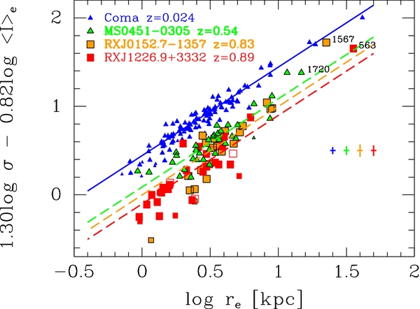
Figure 11. Fundamental Plane for the three clusters and the Coma cluster. Symbols are the same as in Figure 10. The BCG in the three high-redshift clusters are labeled. Blue solid line: best-fit relation for the Coma cluster; green line: best-fit relation for the Coma cluster offset to the median zero point of MS0451.6−0305; orange line: best-fit relation for the Coma cluster offset to the median zero point of RXJ0152.7−1357; red line: best-fit relation for the Coma cluster offset to the median zero point of RXJ1226.9+3332.
Download figure:
Standard image High-resolution image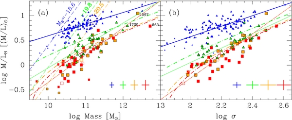
Figure 12. M/L ratios vs. (a) masses and (b) velocity dispersions. Symbols are the same as in Figure 10. Blue solid lines: best-fit relations for the Coma cluster; green solid lines: best-fit relations for the MS0451.6−0305 galaxies; red/orange solid lines: best-fit relations for the RXJ0152.7−1357 and RXJ1226.9+3332 galaxies. Thin colored dashed lines in panel (a) show the approximate magnitude limits for the Coma cluster sample (blue), the MS0451.6−0305 sample (green) and the combined RXJ0152.7−1357 and RXJ1226.9+3332 (red) samples. The thick dot-dashed lines show the predicted location of the relations based on the models by Thomas et al. (2005) for each of cluster redshifts—green: MS0451.6−0305; orange: RXJ0152.7−1357; red: RXJ1226.9+3332.
Download figure:
Standard image High-resolution imageThe samples in two highest redshift clusters RXJ0152.7−0305 and RXJ1226.9+3332 were fit both separately and together. By fitting two parallel relations to the two samples we tested if there were significant zero point offsets between them and found none. Thus, for the purpose of discussing the change in slope of the relations with redshift, we will consider the fits established for the joint sample of the two clusters. The slightly larger sample of RXJ0152.7−1357 and RXJ1226.9+3332 confirms our results from Jørgensen et al. (2006, 2007) of a "steeper" FP at z = 0.86 compared to that of the Coma cluster. The MS0451.6−0305 also shows a steeper FP, but to a lesser extent.
In Figure 12, we show the model prediction from Thomas et al. (2005) for each of the cluster redshifts for models in which high-mass galaxies form the majority of their stars at high redshifts while lower mass galaxies experience later star formation. The models reproduce the general trends of the M/L–mass and M/L–velocity dispersion relations for the intermediate-redshift clusters, though the data show a larger evolution in M/L ratios that predicted by the models, especially for low-mass (low velocity dispersions) galaxies. Thus, in the case of passive evolution this would mean a lower formation redshift than zform = 1.4, as assumed by the models for log σ = 2.1 galaxies. Using the best-fit relations for log σ versus log M/L to determine the differences in log M/L and therefore the formation redshifts we find for log σ = 2.1 (Mass = 1010.55 M☉) a formation redshift of zform ≈ 1.2. At log σ = 2.35 (Mass = 1011.36 M☉) the difference in log M/L corresponds to zform ≈ 2.45. Both of these estimates are based on the fits to the low-redshift sample and the joint sample of the two highest redshift clusters. The fit to the MS0451.6−0305 sample implies lower formation redshifts, ≈0.95 and 1.2 for low and high velocity dispersion galaxies, respectively.
9.3. Line Indices versus Velocity Dispersion
Figure 13 shows the absorption line indices versus the velocity dispersions for the low-redshift sample together with all the intermediate-redshift samples. The relations and zero points are summarized in Table 10.
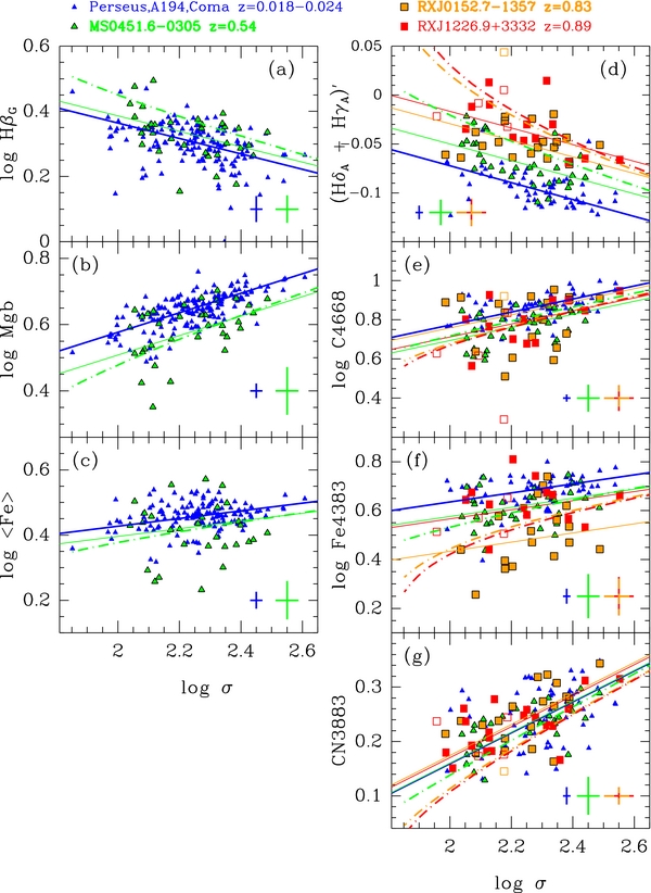
Figure 13. Line indices vs. the velocity dispersions. Blue triangles: the low-redshift comparison sample (Perseus, A194, and Coma); green triangles: MS0451.6−0305 galaxies; orange squares: RXJ0152.7−1357 galaxies; red squares: RXJ1226.9+3332 galaxies. Open points: galaxies with significant [O ii] emission but EW[O ii] ⩽ 5 Å. Typical uncertainties are shown; see Table 19 in Appendix B. We adopt the same uncertainties for RXJ0152.7−1357 as for RXJ1226.9+3332. Solid blue lines: best fits to the low-redshift sample; solid green lines: relations for MS0451.6−0305; solid orange lines: relations for RXJ0152.7−1357; solid red lines: relations for RXJ1226.9+3332. The slopes of the relations determined from the low-redshift sample were adopted. The lines for the intermediate-redshift clusters show the low-redshift relations offset to the median zero points of the intermediate-redshift clusters. The thick dot-dashed lines show the model predictions based on models by Thomas et al. (2005) for cluster redshifts—green: MS0451.6−0305; orange: RXJ0152.7−1357; red: RXJ1226.9+3332.
Download figure:
Standard image High-resolution imageOur data for MS0451.6−0305 allow us to compare the galaxies in this cluster directly with the low-redshift sample using the well-studied indices HβG, Mgb, and 〈Fe〉. There are no significant differences in the slopes of the relations for the low-redshift sample and those for the MS0451.6−0305 sample. Using the median zero points for the cluster, we find that HβG is only marginally stronger in MS0451.6−0305 than in the low-redshift sample, while both Mgb and 〈Fe〉 are weaker at the 3σ–5σ level; see Table 10. The scatter of the relations for Mgb and 〈Fe〉 are two to three times higher for MS0451.6−0305 than found for the low-redshift sample. This difference cannot be explained by higher measurement uncertainties and may indicate that the galaxies in the MS0451.6−0305 sample are more diverse than those in the low-redshift sample.
For RXJ0152.7−1357 and RXJ1226.9+3332 only indices blueward of 4700 Å are available. These indices are also available for MS0451.6−0305 and for the low-redshift samples in Perseus and A194. As for the line indices in the visible, we cannot detect any significant differences of the slopes of the relations for the different clusters. We therefore use the slopes established for the low-redshift sample and determine zero point offsets relative to these and scatter relative to the offset relations. Only the relation for the higher order Balmer lines shows a clear redshift dependence of the zero point with the intermediate-redshift clusters having stronger Balmer lines. In Jørgensen et al. (2005) we found that the RXJ0152.7−0305 galaxies have significantly weaker Fe4383 than the low-redshift sample. The other two clusters do not show significantly weaker Fe4383. All other relations for the metal lines show that the z = 0.5–0.9 clusters follow the same relations as the low-redshift sample with the zero points being within 2σ of each other. The relations for Fe4383 and C4668 show higher scatter in the intermediate-redshift clusters than found for the low-redshift sample, again indicating that the samples in these clusters may be more diverse than our low-redshift comparison sample. The samples in RXJ0152.7−1357 and RXJ1226.9+3332 contain galaxies at larger normalized cluster center distances Rcl R-1500 than the other clusters. We have tested if we in these samples can detect any correlation between Rcl R-1500 and the residuals for the relations between the line indices and the velocity dispersions. We find no significant relations. There are also no significant zero point differences between galaxies at Rcl R-1500 > 1 and those closer to the cluster centers. It may require larger samples in intermediate-redshift clusters, going to larger cluster center distances, to detect any correlations if these are present as they are in low-redshift clusters (Smith et al. 2006).
The model predictions for the passive evolution model from Thomas et al. (2005) are overlaid in all panels in Figure 13. For the Balmer lines, the models predict stronger lines than measured in the galaxies in the intermediate-redshift clusters. Under the assumption of passive evolution, the formation redshifts for these galaxies would have to be higher than assumed by the models. This in turn is inconsistent with the results based on the FP. For the Mgb and 〈Fe〉 indices the passive evolution models reproduce the data well, while for the blue metal indices Fe4383 and CN3883 the models predict larger zero point offsets than measured from the data. For CN3883 in particular the data show no significant zero point offsets. We return to the zero point differences as a function of redshift in the discussion of the passive evolution model in Section 12.3.
10. LINE INDICES AND STELLAR POPULATION MODELS
In this section we use the SSP model predictions and the measured line indices to derive the distributions of ages, metallicities [M/H], and abundance ratios [α/Fe] for each of the clusters. Figures 14 and 15 show the line indices versus each other with SSP models from Thomas et al. (2011) overlaid.
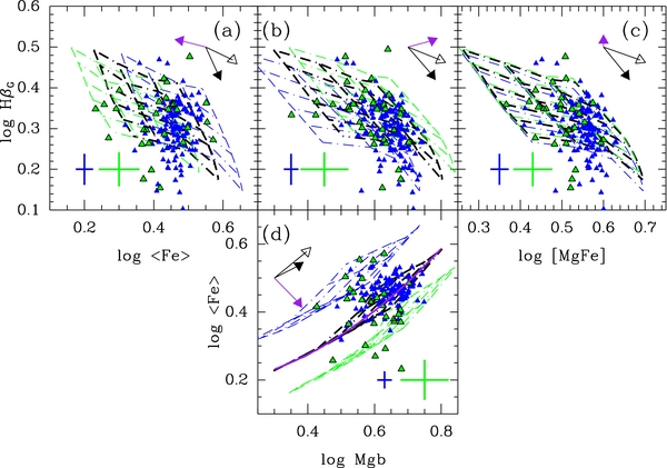
Figure 14. Line indices in the visible vs. each other for the low-redshift sample and MS0451.6−0305. Blue triangles: the low-redshift comparison sample (Perseus, A194, and Coma); green triangles: MS0451.6−0305 galaxies. Typical uncertainties are shown; see Table 19 in Appendix B. Model grids from Thomas et al. (2011) are overlaid. Blue: [α/Fe] = 0; black: [α/Fe] = 0.3; green: [α/Fe] = 0.5. Models are shown for ages from 2 Gyr to 15 Gyr and [M/H] from −0.33 to 0.67. The arrows show the model predictions for Δlog age = 0.3 (solid); Δ[M/H] = 0.3 (open); Δ[α/Fe] = 0.3 (purple). Solid purple line in panel (d): second-order approximation to the model for [α/Fe] = 0.3 used for the determination of [α/Fe]; see Section 10.
Download figure:
Standard image High-resolution image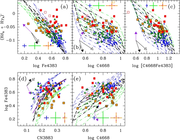
Figure 15. Line indices in the blue vs. each other. Symbols are the same as in Figure 13. Typical uncertainties are shown; see Table 19 in Appendix B. We adopt the same uncertainties for RXJ0152.7−1357 as for RXJ1226.9+3332. Model grids from Thomas et al. (2011) are overlaid. Blue: [α/Fe] = 0; black: [α/Fe] = 0.3; green: [α/Fe] = 0.5. Models are shown for ages from 2 Gyr to 15 Gyr and [M/H] from −0.33 to 0.67. The arrows show the model predictions for Δlog age = 0.3 (solid), Δ[M/H] = 0.3 (open), and Δ[α/Fe] = 0.3 (purple). Solid purple line in panel (d): second-order approximation to the model for [α/Fe] = 0.3 used for the determination of [α/Fe]; see Section 10.
Download figure:
Standard image High-resolution imageThe stellar population models in general span the range of the visible indices (HβG, Mgb, 〈Fe〉) fairly well, though both the low-redshift sample and the MS0451.6−0305 sample contain galaxies with weaker HβG than predicted by the models. These galaxies do not have detectable emission lines, though very low level emission fill-in of the Hβ line cannot be ruled out. The indices [MgFe] and HβG make it possible to derive ages and metallicities [M/H] without significant dependence on the assumption about [α/Fe]. The Mgb versus 〈Fe〉 diagram offers the possibility of estimating the abundance ratio [α/Fe] independent of age and total metallicity. We return to this later in this section.
For the blue indices the models give a reasonable match to the strengths of C4668, CN3883, Fe4383, and (HδA + HγA)', though a significant number of galaxies in the high-redshift cluster RXJ1226.9+3332 have strong (HδA + HγA)' while also having strong Fe4383, and thus being in an area of the parameter space not covered by the models (see Figure 15(a)). From the indices [C4668 Fe4383] and (HδA + HγA)' we can derive ages and metallicities while limiting dependence on the assumption regarding [α/Fe]. CN3883 versus Fe4383 offers a similar possibility of estimating [α/Fe] as the (Mgb,〈Fe〉) diagram. However, CN3883 is only a tracer of [α/Fe] to the extent that carbon and nitrogen enhancements follow the [α/Fe] abundance ratio.
In order to establish the distribution of mean ages, mean metallicities [M/H], and mean abundance ratios [α/Fe], we proceed as follows. We use a Balmer line index and together with a combination metal index independent of [α/Fe] to derive mean ages and mean metallicities [M/H] by interpolation in the model grid from Thomas et al. (2011). We choose to use a model grid for [α/Fe] = 0.25 for this, but because of the indices used this choice is not critical. In the visible we use (HβG,[MgFe]), while in the blue we use (HδA + HγA)',[C4668 Fe4383]). The resulting cumulative distributions are shown in Figure 16. To derive the abundance ratio [α/Fe] we use Mgb versus 〈Fe〉 in the visible and CN3883 versus Fe4383 in the blue. For both diagrams we fit a second-order polynomial to the model points for [α/Fe] = 0.3. Then we determine the distance from each data point to this model approximation, measured along the vector of the [α/Fe] dependency of the indices. The polynomials and the vectors are shown in purple in Figures 14(d) and 15(d). The vector distance is then converted to [α/Fe] using the coefficients for the model fits in Table 9. The resulting distributions of [α/Fe] are shown in Figure 16.
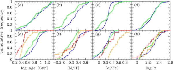
Figure 16. Cumulative distributions of age, [M/H], and [α/Fe]. The ages and [M/H] are derived by inverting (HβG, [MgFe]) (a and b) or ((HδA + HγA)', [C4668 Fe4383]) ((e)–(f)), under the assumption that [α/Fe] = 0.25. The abundance ratios [α/Fe] are derived from (Fe,Mgb) or (Fe4383,CN3883); see Section 10. Panels (d) and (h) show the distributions of the velocity dispersion of the samples used for the determination of the ages, metallicities, and abundance ratios; see the text for discussion. Blue line: low-redshift sample; green line: MS0451.6−0305; orange line: RXJ0152.7−1357; red line: RXJ1226.9+3332.
Download figure:
Standard image High-resolution imageIndependent of the absolute accuracy of the models, these estimates of [α/Fe] convert the 2D parameter spaces of (Mgb,〈Fe〉) and (CN3883,Fe4383) into 1D parameter space of the estimated [α/Fe] from which we can test with better accuracy if the distributions vary from cluster to cluster. The samples are in general too small to be suitable for a 2D Kolmogorov–Smirnov test. It should also be noted that the measurements should be considered relative, rather than absolute measurements, and that deriving [α/Fe] from the blue indices assumes that the carbon and nitrogen abundances track the α-element abundances.
The age distributions derived from the visible indices show an insignificant age different between the low-redshift sample and the MS0451.6−0305 sample, as also found when using the HβG versus the velocity dispersion relation. The age distributions derived from the blue indices show lower median ages for the intermediate-redshift clusters, restating the result from the (HδA + HγA)' versus velocity dispersion relation.
The distributions of [M/H] derived from the blue indices show that the distributions for RXJ0152.7−1357 and RXJ1226.6+3332 are not significantly different from the distribution for the low-redshift sample. For MS0451.6−0305 the distribution of [M/H], whether derived from the visible or from the blue indices, shows a significantly lower metallicity than the low-redshift sample. We tested the significance of these differences using a 1D Kolmogorov–Smirnov test and find probabilities that the [M/H] distributions for the MS0451.6−0305 and the low-redshift sample are drawn from the same parent distribution of 1% and <0.2% when using the visible and the blue indices, respectively. The difference in [M/H] is ≈0.2 dex.
The distributions of [α/Fe] from the blue indices show that the distributions for MS0451.6−0305 and RXJ1226.6+3332 are not significantly different from the distribution for the low-redshift sample. For RXJ0152.7−1357 significantly higher [α/Fe] are found, as we also noted in Jørgensen et al. (2005). The median difference between RXJ0152.7−1357 and the low-redshift sample is ≈0.3 dex. A 1D Kolmogorov–Smirnov test shows that the probability the two distributions are drawn from the same parent distribution is ≪0.01%.
Ages, [M/H], and [α/Fe] have been found to correlate with the velocity dispersions (e.g., Thomas et al. 2010). Our current samples at intermediate redshifts are not large enough to detect these correlations as they have quite high scatter. However, to ensure that the cluster differences in distributions found for [M/H] and [α/Fe] are not simply caused by differences in the distributions of the velocity dispersions we also show the distributions of the velocity dispersions for the galaxies included in the tests (see Figures 16(d) and (h)). For the distributions based on the blue indices there is a tendency for the intermediate-redshift samples to contain a larger fraction of low velocity dispersion galaxies than is the case for the low-redshift comparison sample. To correct for the possible effect introduced by these differences, we normalized the derived ages, [M/H], and [α/Fe] to the median velocity dispersion of the sample (log σ = 2.24), using the relations between velocity dispersion, age, [M/H], and [α/Fe] given by the two studies by Thomas and collaborators (Thomas et al. 2005, 2010). We then repeated the Kolmogorov–Smirnov tests described above. With these normalized values, the probabilities that the [M/H] distributions for the MS0451.6−0305 and the low-redshift sample are drawn from the same parent distribution is 0.6%–1% and 2.5% when using the visible and the blue indices, respectively. When comparing the distributions of the normalized [α/Fe] values for RXJ0152.7−1357 and the low-redshift sample, the Kolmogorov–Smirnov test shows that the probability the two distributions are drawn from the same parent distribution is ≪0.01%. Thus, both results based on the "raw" measurements of [M/H] and [α/Fe] are maintained when correcting for the correlation of the parameters with velocity dispersion.
Finally, we used the models from Thomas et al. (2011) to investigate if the carbon or nitrogen enhanced stellar populations would be consistent with the data. If we use the models with [C/α] = 0.3 then C4668 is predicted significantly stronger than observed. The dependency of C4668 on [C/α] is so strong (Table 9) that any carbon enhancement, [C/α], of more than about 0.1 dex affecting all the galaxies can be ruled out if the total metallicities are above [M/H] = -0.33. The model with [N/α] = 0.3 (and [α/Fe] = 0.3) may be a possibility of explaining the strong CN3883 indices for some galaxies, though a general enhancement of nitrogen [N/α] of more than about 0.1 dex will move the location of the models off the distribution of data in C4668 versus CN3883. Based on these considerations, we do not consider the carbon or nitrogen enhanced models (above the α-enhancement) to provide a viable modeling of the line indices. However, it should still be kept in mind that using C4668 and CN3883 in place of Mgb will provide information about carbon and nitrogen, rather than the α-element magnesium, and only to the extent that enrichment in these elements track each other can the indices be used interchangeable.
In summary, the line indices show that (1) the median age varies with redshifts of the clusters, (2) the MS0451.6−0305 galaxies have [M/H] ≈ 0.2 dex lower than the low-redshift sample, and (3) the RXJ0152.7−1357 galaxies have [α/Fe] ≈ 0.3 dex higher than the low-redshift sample. The latter two points are in disagreement with a passive evolution model. We will return to this in the discussion in Section 12.
11. EVOLUTION AS A FUNCTION OF REDSHIFT
To study the evolution of the galaxies both as a function of redshift and as a function of velocity dispersion (or mass), we divide the samples in each cluster into two subsamples according to velocity dispersions. We could instead have divided according to the mass. However, since mass and velocity dispersion are tightly correlated and that relation is the same for all clusters in the sample (see Section 9.1) the two choices are equivalent. The two subsamples are defined as follows:
The limit in log σ is equivalent to log Mass = 11.0. As such the high velocity (mass) sample is equivalent to the samples of high-mass galaxies for which the evolution with redshift has been studied by other groups, e.g., van Dokkum & van der Marel (2007). The sample limits in log σ also match those used in the analysis of the EDisCS data by Sánchez-Blázquez et al. (2009). Galaxies with log Mass < 10.3 were excluded from the analysis; cf. Section 8. Each of the subsamples contains roughly half of the full sample in each cluster. The approximate average velocity dispersions for galaxies in the two subsamples are log σ = 2.1 and 2.35.
We use the scaling relations for the low-redshift sample as the reference; see Table 10. For each of the two subsamples in each cluster, and for the full cluster sample, we determine the zero point differences to the scaling relations established for the low-redshift sample. The values for the full cluster samples are listed in Table 10.
Figure 17 shows the zero point differences versus the redshifts of the clusters. The curves in the figure are models for passive evolution with formation redshifts between zform = 1.2 and 4.0, based on the SSP models from Maraston (2005) and Thomas et al. (2011). The zero point differences for the M/L ratios as a function of redshift in general indicate a lower formation redshift than found from the line indices. We discuss this in detail in Section 12.3.
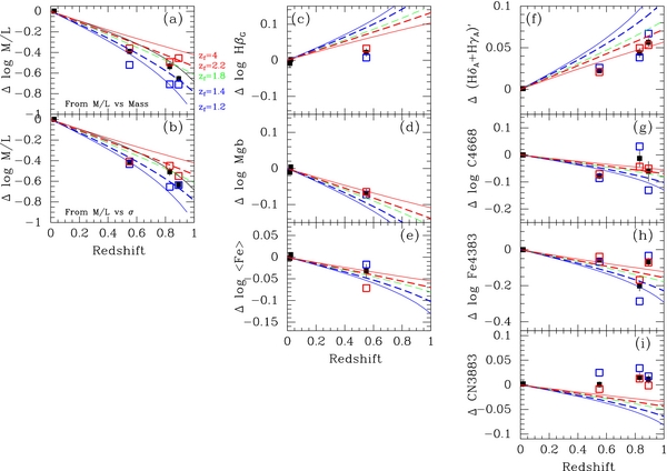
Figure 17. Zero point differences of the scaling relations vs. redshift for each of the clusters, and for the two subsamples within each cluster. Black: all galaxies in a given cluster with the error bars showing the random uncertainties only—cf. Equation (7); red: galaxies with log σ ⩾ 2.24 or for panel (a) log Mass ⩾ 11; blue: galaxies with log σ < 2.24 or for panel (a) log Mass < 11. In all cases the zero point difference is derived as Δzp = zphigh − z − zplow − z, where the zero points for the full cluster samples are listed in Table 10. Predictions for passive evolution models are overplotted. Solid blue line: Salpeter IMF, zform = 1.2; dashed blue line: Salpeter IMF, zform = 1.4; dashed green line: Salpeter IMF, zform = 1.8; dashed red line: Salpeter IMF, zform = 2.2; solid red line: Salpeter IMF, zform = 4.0. Formation redshifts of zform = 1.4 and 2.2 correspond to the low mass (velocity dispersion) and high mass (velocity dispersion) formation redshifts predicted by Thomas et al. (2005). In panels (a) and (b) the solid black lines show the prediction for a steeper IMF (x = 2.3) and zform = 1.2 using models from Vazdekis et al. (2010).
Download figure:
Standard image High-resolution imageTo directly estimate the mean ages, metallicities, and abundance ratios for the subsamples, we use the scaling relation zero points for the subsamples for each cluster together with the slopes for the low-redshift sample to determine the strength of each line at velocity dispersions of log σ = 2.1 and 2.35, respectively. Using the zero points for the full sample in each cluster together with the slope for the low-redshift sample, we also determine the strength of each line at velocity dispersions of log σ = 2.24. These three velocity dispersion values correspond to masses of log Mass = 10.55, 11.0 and 11.36, respectively. Thus, for each cluster we have three mean values of each line index, tracing the dependence on the velocity dispersion (or alternatively the mass).
We have then used the models to estimate the mean age and [M/H], and [α/Fe] corresponding to the mean values for the line indices, using the same technique as for the individual galaxies (see Section 10). This leads to two sets of values for (age, [M/H], [α/Fe]) for each sample in the low-redshift clusters and MS0451.6−0305. One set comes from using (HβG, Mgb, 〈Fe〉), while the other set comes from using ((HδA + HγA)', C4668, Fe4383). For the intermediate-redshift clusters RXJ0152.7−1357 and RXJ1226.9+3332 only the latter set of values can be derived.
In Figure 18 we show the derived parameters as a function of redshift. This figure shows the same general trends as are evident in the detailed distributions of the parameters (Figure 16). The ages when derived from the blue indices vary with redshift, in agreement with a passive evolution model with a formation redshift of zform ≈ 1.8 with some indication that the formation redshift is higher for higher mass galaxies than for the lower mass galaxies. For MS0451.6−0305 the ages derived from the visual indices are higher than those derived from the blue indices. However, the difference between the ages for the MS0451.6−0305 samples and the low-redshift samples are independent of which set of indices are used. In both cases the ages for the low-redshift samples are lower than expected from the passive evolution models. We return to this issue in the discussion of the passive evolution model in Section 12.3.
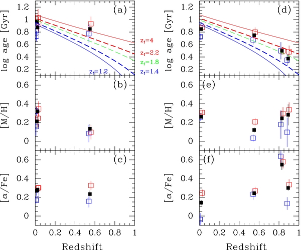
Figure 18. Estimates of age, [M/H], and [α/Fe] derived from the mean line index values. The ages and [M/H] are derived by interpolation in the models for (HβG, [MgFe]) (a and b) or ((HδA + HγA)', [C4668 Fe4383]) ((d)–(e)), under the assumption that [α/Fe] = 0.25. The abundance ratios [α/Fe] are derived from (Fe,Mgb) or (Fe4383,CN3883), see Section 11. The error bars correspond to the scatter within the samples of the indices used for the estimates. Symbols are the same as in Figure 17. Expected ages for passive evolution models are shown in panels (a) and (d)—solid blue line: Salpeter IMF, zform = 1.2; dashed blue line: Salpeter IMF, zform = 1.4; dashed green line: Salpeter IMF, zform = 1.8; dashed red line: Salpeter IMF, zform = 2.2; solid red line: Salpeter IMF, zform = 4.0. Formation redshifts of zform = 1.4 and 2.2 correspond to the low mass (velocity dispersion) and high mass (velocity dispersion) formation redshifts predicted by Thomas et al. (2005).
Download figure:
Standard image High-resolution imageThe metallicity [M/H] for MS0451.6−0305 whether derived from visible or blue indices, is ≈0.15 dex below that of the low-redshift sample. Using the uncertainties derived on [M/H] and based on the scatter in the samples, the difference is significant at the 4σ level. Using the blue indices, all three intermediate-redshift clusters show that the low-mass galaxies are less metal rich than the high-mass galaxies. The mean difference is ≈0.25 dex. RXJ0152.7−1357 is found to have higher [α/Fe] than the rest of the clusters, ≈0.3 dex, in agreement with the result from the distribution of the values for the individual galaxies. The difference is significant at the 5σ level.
12. DISCUSSION
In this discussion, we initially assume that the galaxies in the high-redshift clusters are the progenitors of the low-redshift sample and that at each redshift they represent a stage in the evolution that early-type galaxies have to pass through. Specifically, we assume that the galaxies in these clusters have the similar evolutionary histories, as a function of velocity dispersion (or mass), and that they travel along similar evolutionary paths to reach the same properties at the present.
The issues we will consider are as follows: (1) the effect of selection effects; (2) possible non-homology among the E/S0 galaxies; (3) age effects, specifically testing the model of passive evolution; (4) effects of the assumed IMF; and (5) metallicity and abundance ratio differences with redshift or among clusters. Each of these is discussed in the following subsections.
12.1. Selection Effects
Before we discuss the physical effects, it is important to understand to what extent the results may be affected by selection effects. The spectroscopic sample selection was described in Section 3.2. Most important for the current discussion is that each cluster sample has a luminosity limit but that high-redshift samples are not complete to that limit. In addition, only galaxies with early-type morphologies and EW[O ii] ⩽5 Å are included in the sample.
We focus on how the selection effects may affect the results for the FP offset and slope. In Jørgensen et al. (2006, 2007) we presented results of a bootstrap simulation, drawing samples of the same size as the high-redshift sample from both the Coma cluster sample and the high-redshift sample, and fitting these. The results showed a significance of the slope difference at the 96%–98% level. However, one could also argue that the difference is slope may be caused by systematically missing fainter galaxies in the high-redshift sample at a given mass.
We tested this by determining if the difference in slope depends on the chosen mass limit. Due to the slope of the luminosity limit lines in the M/L–mass plane (Figure 12(a)) the effect of the limiting magnitude will decrease with increasing mass limits. The test was done using the joint sample of the galaxies in RXJ0152.7−1357 and RXJ1226.9+3332, since our analysis of the FP shows that these two samples follow the same FP. We applied lower limits in log Mass to both this sample and the Coma sample from 10.4 to 11.3 in steps of 0.1 and refit each of these subsamples. Figure 19 shows the coefficient of log M/L in the mass–M/L ratio as a function of the value of the applied mass limit. For limits of log Mass = 10.8 or smaller the difference in the slope for the intermediate-redshift sample and the Coma sample is significant approximately at the same level as for the full sample (also shown in the figure at the limit of log Mass = 10.3). In all cases the slope difference is about 0.32. If the sample is limited at log Mass = 10.9 or higher, the slope difference is about 0.16, and the uncertainties are larger due to the smaller samples. Thus, formally the slope difference is not statistically significant for limits of log Mass ⩾10.9. However, given that the slope difference is very stable for sample limits of log Mass ⩽10.8 we conclude that the result is not an effect of the selection effects due to the luminosity limits of the data.
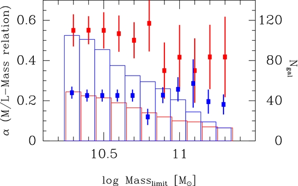
Figure 19. Slope α of the relation between log M/L and log Mass as a function of the adopted limit in log Mass. Red boxes: coefficient for fit to the joint sample of RXJ0152.7−1357 and RXJ1226.9+3332. Blue boxes: coefficient for fit to the Coma cluster sample, for clarity slightly offset from the high-redshift sample in log Mass. The histograms show the number of galaxies included in the fits for each of the limits in log Mass; red: the sample of RXJ0152.7−1357 and RXJ1226.9+3332; blue: the Coma cluster sample. The difference in slope is significant for all limits of log Mass = 10.8 or smaller.
Download figure:
Standard image High-resolution image12.2. Non-homology among the E/S0 Galaxies
The mass determination used here, Mass = 5reσ2 G−1 (Bender et al. 1992), assumes homology among the galaxies. The current data set does not offer the possibility of explicitly testing the effect of possible non-homology among the galaxies. van Dokkum et al. (2010) propose that a better mass estimate may be achieved by using the Sérsic (1968) index, n, to determine the coefficient in the mass determination. Using their equation the coefficient would be 3.24 at n = 2 and 2.58 at n = 6, rather than the constant value of 5 that we have used. If we determine the masses using the equation from van Dokkum et al. (2010) and then refit the M/L–mass relation then we find for the sample of the two highest redshift clusters

Comparing to the M/L–mass relation for the two highest redshift clusters listed in Table 11, we conclude that this different mass estimate does not result in a significantly different slope for the relation.
Cappellari et al. (2006) found from the integral-field-unit (IFU) data of early-type galaxies that any non-homology is an insignificant contribution to the difference between the FP slope and the slope expected from the virial relation, thus leading these authors to conclude that the difference is due to real M/L variations. The same conclusion is reached by Bolton et al. (2007) using SDSS data to derive galaxy masses based on strong gravitational lensing. Cappellari et al. (2006) also conclude that the approximation Mass = 5reσ2/G provides a reasonable mass estimate when data are not available for more detailed modeling. Finally, we note that there is no significant correlation between M/L–mass relation residuals and the Sérsic index, using the relations listed in Table 11. Since the slope of the M/L–mass relation is the same using mass estimates taking the Sérsic index into account compared to using our simpler approximation, and the low-redshift IFU studies confirm that the simpler approximation is valid, we will in the following discussion assume that the galaxies in our sample form a homologous class of galaxies.
12.3. Passive Evolution
The simplest of models for galaxy evolution is passive evolution of the stellar populations over the redshift interval covered by the data. The FP (Figure 11), the M/L–mass relation and the M/L–velocity dispersion relation (Figure 12) are consistent with passive evolution with the low-mass (low velocity dispersion) galaxies being younger than those of higher mass (higher velocity dispersion). We discussed this result in detail in Jørgensen et al. (2006, 2007) for the two highest redshift clusters RXJ0152.7−1357 and RXJ1226.9+3332. The data for MS0451.6−0305 are also consistent with this interpretation. The zero point differences for the subsamples described in Section 11 implies a formation redshift for the low velocity dispersion galaxies (log σ = 2.1; Mass = 1010.55 M☉) of zform = 1.24 ± 0.05. The uncertainty takes into account only the scatter of the data relative to the relations. For the high velocity dispersion galaxies (log σ = 2.35; Mass = 1011.36 M☉) we find zform = 1.95+0.30−0.20. The result for the high velocity dispersion galaxies can directly be compared to the result from van Dokkum & van der Marel (2007) who find zform = 2.23+0.24−0.18, before correcting for progenitor bias. Half of the difference between our result and that of van Dokkum & van der Marel is due to a difference in the assumed dependency of the M/L on the age of the stellar population. As such the two results agree within the uncertainties.
The other major age indicator is the strengths of the Balmer lines. The Balmer lines for the intermediate-redshift clusters are too weak compared to what is predicted by the models for passive evolution with formation redshifts as derived from the M/L ratios. We focus here on (HδA + HγA)', which we have measured for all the clusters. As we do not detect a change in slope of the (HδA + HγA)'–velocity dispersion relation with redshift, we only give the formation redshift for the full sample. For the z = 0.8–0.9 clusters we find zform > 2.8. This is consistent with the result from Kelson et al. (2001) who finds zform > 2.4 or >2.9 depending on which SSP model is used for the interpretation. The formation redshift for the galaxies in MS0451.6−0305 would have to be even higher; see Figure 17(f), for the galaxies to be able to passively evolve into their low-redshift counterparts.
If the offset and slope differences of the M/L–mass relation are purely due to age differences, and therefore differences in formation redshift as a function of mass, we also expect to see offsets and (to lesser extent) slope differences in the relations between the metal line indices and the velocity dispersion. As the metal lines are predicted to be weaker with younger ages, we expect the intermediate-redshift samples to show offsets to weaker metal lines. Figure 17 shows the zero points together with the model predictions from passive evolution models. The measured offsets do not allow a straightforward interpretation within the passive evolution model or a conversion of the offsets to a formation redshift. In general, the offsets are smaller than predicted from the passive evolution model from Thomas et al. (2005). In particular, all the intermediate-redshift clusters have significantly stronger CN3883 than expected from the passive evolution model. CN3883 for the z = 0.8–0.9 clusters represent 4σ deviations from the model with zform = 4. If we were to adopt the age dependence of CN3883 from the model spectra by Maraston & Strömbäck (2011), the difference would be even larger due to the stronger age dependence predicted for CN3883; see Section 6.
Part of the difference between the formation redshifts as found from the FP and from the high-order Balmer lines (HδA + HγA)' may be due to different sensitivity in the two methods to progenitor bias. We found that the mean ages for the low-redshift samples are lower than expected from the passive evolution model (Figure 18) and that some of the galaxies have ages too low for them to be the progenitors of the intermediate-redshift sample galaxies. For example, roughly 40% of the low-redshift sample have ages of less than ≈7.1 Gyr, which is the look-back time corresponding to z = 0.86. We have performed a simple test for the effect of the progenitor bias, by excluding these galaxies from the estimates of the mean ages based on the blue indices. These results result in a mean age for the low-redshift sample of ≈10 Gyr, and bring the data in agreement with the passive evolution model (Figure 18). However, excluding these galaxies from the determination of the zero points for the scaling relations for M/L and (HδA + HγA)' versus velocity dispersion lead to only insignificant changes. It also does not bring the zero point differences between the low-redshift sample and the intermediate-redshift samples for these scaling relations into agreement with each other.
As a different way of illustrating the disagreement between the FP and the strength of (HδA + HγA)' we use the SSP models (Maraston 2005) to predict the stellar M/L ratios, given the ages and metallicities derived from the line indices. As the possible dependency of the M/L ratios on the abundance ratios [α/Fe] has not been modeled, we will assume that it is insignificant. In Figure 20 we show the resulting M/L ratio versus velocity dispersion. In this view there is no change in the slope with redshift. We fit the samples with a set of parallel lines as shown in the figure. The zero point differences agree with the high the formation redshift found from (HδA + HγA)' versus velocity dispersion. Formally we find zform > 4. Taken at face value, Figure 20 compared with the FP (Figure 12) indicates that the stellar M/L ratios change significantly less than the dynamical M/L ratios since z ≈ 0.9. We note that Toft et al. (2012) found a similar difference in the change of M/L ratios for massive galaxies between z ≈ 2 and the present. These authors speculated that the effect may be due to a change in the dark matter content. In our view, it is premature to conclude that a change in dark matter content can lead to the effect we find for the low-mass galaxies in these intermediate-redshift clusters. However, we plan to return to this issue using our full galaxy sample in the GCP.

Figure 20. Stellar M/L ratio as derived from the ages and metallicities resulting from (HδA + HγA)' and [C4668Fe4383] vs. the velocity dispersions. Symbols are the same as in Figure 15. The solid lines are best-fit relations assuming the clusters follow relations with identical slopes (blue: low-redshift sample; green: MS0451.6−0307; orange-red: RXJ0152.7−1357 and RXJ1226.9+3332 treated as one sample). Dashed blue line: for reference the fit to the Coma cluster sample using dynamical M/L ratios (Figure 12(b)). The zero point differences indicate formation redshifts of zform > 4; see the text.
Download figure:
Standard image High-resolution imageEven if the difference in the formation redshift derived from the FP and from (HδA + HγA)' versus velocity dispersion may be consolidated by invoking a change in dark matter content, passive evolution implies that the metallicity [M/H] and the abundance ratio [α/Fe] do not vary from cluster to cluster. However, both the distributions of the estimates of [M/H] and [α/Fe] for the individual galaxies (Figure 16) and the mean values derived from the mean indices (Figure 18) show that the mean [M/H] for MS0451.6−0305 is 0.2 dex below the other clusters, while the mean [α/Fe] for RXJ0152.7−1357 is 0.3 dex above the other clusters. Both of these results contradict the model of passive evolution.
In summary, it is not possible within the current SSP models using one IMF slope (Salpeter) for all the galaxies to find a passive evolution model that agrees with the data within the measurement uncertainties. While the slope changes with redshift of the M/L–mass and M/L–velocity dispersion relations indicate a difference in formation redshift for low- and high-mass galaxies, this is not consistent with the (HδA + HγA)' data for the intermediate-redshift clusters. It is also inconsistent with the strong metal lines in general found for all the intermediate-redshift clusters. Further, the formation redshift implied by the M/L ratios is significantly lower than found from the higher order Balmer lines. This result does not change even if we remove all galaxies in the low-redshift sample with ages too young to have progenitors included in the intermediate-redshift samples. Future investigations may show if these two results can be consolidated by the presence of a change in the dark matter content, primarily for the low-mass galaxies, between z ≈ 0.9 and the present.
12.4. Initial Mass Function
We have investigated what effect differences in the IMF as a function of galaxy mass would have on the observed evolution. For simplicity we assume that the galaxies evolve passively, but that the IMF slope depends on the galaxy mass or the velocity dispersion. This idea is based on recent results indicating that at low redshift higher mass galaxies may have steeper IMFs than the low-mass galaxies (van Dokkum & Conroy 2010, 2011; Conroy & van Dokkum 2012a, 2012b; Cappellari et al. 2012). However, an apparently contradicting result was found by van Dokkum (2008) for the evolution of the IMF, showing that a bottom-light IMF for high-mass galaxies can explain the redshift evolution of both the FP zero point and the (U − V) colors.
To investigate the effect of differences in the IMF between low- and high-mass galaxies we used the models from Vazdekis et al. (2010). Using a Kroupa (2001) "universal" IMF instead of a Salpeter IMF leads to the same age dependence on the M/L ratio, while there naturally is a zero point difference in the resulting M/L ratios for the two IMFs due to the presence of more low-mass stars in models using a Salpeter IMF than those using a Kroupa IMF. However, the evolution in the M/L ratio over the length of time probed by our data is not significantly different for the two choices of IMF.
We then tested the difference between using a Salpeter IMF with x = 1.3 as is used in the default models and a steeper and therefore dwarf-rich IMF with a slope of x = 2.3. The result is shown in Figure 17 as the expected evolution of the M/L ratio. With the dwarf-rich IMF (x = 2.3) the M/L ratio evolves much slower for a given formation redshift. If we hypothesize that the IMF slope is x = 1.3 for the low-mass galaxies and increases slowly to x = 2.3 for the high-mass galaxies, then it would reproduce the change in slope for the M/L–mass relation (and the FP) with redshift and lead to a formation redshift of z ≈ 1.2 for all the galaxies. The high-order Balmer lines are not significantly affected by the slope of the IMF (Vazdekis et al. 2010). While we in principle can find a solution with a mass-dependent slope of the IMF that will mostly remove the age differences between low- and high-mass galaxies, the result is that their luminosity weighted mean ages are all fairly young, about 2 Gyr for the z = 0.8–0.9 galaxies and about 4 Gyr for the z = 0.54 galaxies. The model predictions for strengths of the higher order Balmer line for such young ages are in disagreement with our data, and would also predict a much larger change in the strength of these lines with redshift than seen from the data; see Figure 17(f). Thus, a simple model where the IMF slope depends on the galaxy masses (or velocity dispersions) does not seem to be viable solution to a consistent model for the observed evolution of the zero points of the M/L–mass relation and the (HδA + HγA)'–velocity dispersion relation, under the assumption of otherwise passive evolution. This does not rule out that there could be IMF variations as a function of galaxy masses in addition to more complex models for the galaxy evolution.
12.5. Metallicities and Abundance Ratios
We now turn to the possible differences in metallicities and abundance ratios. The results in Sections 10 and 11 indicate that the cluster MS0451.6−0305 has [M/H] approximately 0.2 dex lower than the other clusters, while RXJ0152.7−1357 has [α/Fe] approximately 0.3 dex higher than the other clusters. The results indicate that passive evolution is too simple a model to explain the data.
It may be possible to envision that the galaxies in these clusters can evolve into their low-redshift counterparts in the time available. For MS0451.6−0305 this could happen through additional star formation to increase [M/H], as long as such new star formation does not lead to ages younger than expected at redshift zero. For RXJ0152.7−1357 a significant change in [α/Fe] may only be possible through merging of the early-type galaxies with lower [α/Fe] galaxies that are not part of the present sample. Thus, these galaxies have to be either spiral galaxies, galaxies with significant emission, or galaxies fainter than the sample limit. In the first two cases, the galaxies are expected to contain younger stellar populations than the early-type galaxies in our samples, and the merger products will therefore have younger ages than if the early-type galaxies evolved passively. Any merger scenario also has to maintain the relation between sizes and masses, as we detect no evolution in this relation; cf. Section 9.1.
Additional star formation and/or mergers in some clusters and not in others then lead to different paths of evolution for the early-type galaxies in intermediate-redshift clusters in order to reach the properties of the low-redshift counterparts and one has to ask what the underlying reason for this may be.
Of the clusters in the present sample RXJ0152.7−1357 has the clearest evidence for substructure; see Sections 2 and 7. The difference in evolutionary path may be related to the interactions of the galaxies with the intracluster gas as the two substructures interact. This idea is supported by the results from Demarco et al. (2010) who find that the details of the stellar populations appear related to the local cluster density. In particular, they find that their stacked spectrum of galaxies from low-density environment has weaker Fe4383 than the rest of the galaxies. The cluster MS0451.6−0305 is significantly more massive than the other clusters. It may be that the cluster environment in this case led to a truncated star formation history such that the resulting early-type galaxies have higher ages and lower [M/H] than expected if one just evolved RXJ1226.9+3332 passively to z = 0.54. This view is supported by the results from Moran et al. (2007a) based on their analysis of the D4000 break and presence (or rather absence) of emission lines in a very large sample of galaxies in the cluster. Moran et al. (2007a) also studied another rich intermediate-redshift cluster (CL0024+1654) and found that a different star formation history for that cluster best explained the data, indicating that cluster-to-cluster differences among rich clusters are present at z ≈ 0.4–0.5.
Even with surveys like the NOAO Fundamental Plane Survey (Smith et al. 2004, 2006; Nelan et al. 2005) our knowledge of possible cluster-to-cluster variations in rich low-redshift clusters (z ⩽ 0.1) is limited. The X-ray catalog from Piffaretti et al. (2011) contains 26 clusters at z ⩽ 0.1 with X-ray luminosities at least as high as that of the Coma cluster. Those with z ⩽ 0.067 are also included in the NOAO FPS sample. However, the published analysis of these data does not address possible cluster-to-cluster differences. Thus, it cannot be ruled out that there are cluster-to-cluster differences among the most massive galaxy clusters.
13. CONCLUSIONS
We have presented redshifts, velocity dispersions, and absorption line indices for 102 cluster galaxies at z > 0.5. Together with our previously published data for an additional 29 galaxies, this represents the largest galaxy sample to date at z > 0.5 for which velocity dispersions and line indices are determined for individual galaxies based on spectra with S/N ⩾ 20 per Å in the rest frame. We used publicly available HST/ACS imaging to derive effective radii and surface brightnesses for the sample galaxies. We have established the size–mass and size–velocity dispersion relations, the FP, the M/L–mass, and the M/L–velocity dispersion relations, and scaling relations between line strengths and velocity dispersions as a function of redshift. From the location of the galaxies in index-versus-index parameter space compared to predictions from SSP models we have assessed variations in ages, [M/H], and [α/Fe] among the clusters and as a function of redshift. Our main conclusions are as follows.
- 1.The sample shows no significant evolution of galaxy size or velocity dispersion at a given mass between z = 0.9 and the present.
- 2.We confirm the change in the slope of the FP and M/L–mass relation as a function of redshift with the slope being steeper at higher redshift than at z = 0. The original result was in our study of the two high-redshift clusters RXJ0152.7−1357 and RXJ1226.9+3332 (Jørgensen et al. 2006, 2007). In this paper we have added MS0451.6−0305 at z = 0.54. This cluster follows relations with slopes between those of RXJ0152.7−1357 and RXJ1226.9+3332 and that of the low-redshift reference sample. The FPs for all the clusters are consistent with passive evolution with formation redshifts depending on the mass (or alternatively on the velocity dispersion), such that low-mass galaxies have a more recent formation redshift than that of higher mass galaxies. Under the assumption of passive evolution we find that at a velocity dispersion of σ = 125 km s−1 (Mass = 1010.55 M☉) the formation redshift is zform = 1.24 ± 0.05, while at σ = 225 km s−1 (Mass = 1011.36 M☉) zform = 1.95+0.3−0.2.
- 3.The scaling relations for the line indices cannot easily be reconciled with the results from the FP and M/L–mass relation for the clusters studied. In particular, in the intermediate-redshift clusters (1) the Balmer lines are too weak and their scaling relations with the velocity dispersion do not undergo the slope changes with redshift as one would expect if the M/L–mass zero point differences and slope change are due to age differences only. Interpreting the difference in the higher order Balmer lines between the intermediate-redshift clusters and the low-redshift sample within the model of passive evolution leads to a formation redshift zform > 2.8. (2) The metal lines are in general stronger than expected from the predictions for passive evolution, and we find no significant changes with redshift in the slopes of the scaling relations between metal line indices and the velocity dispersion.
- 4.Using stellar M/L ratios based on the ages and metallicities derived from the high-order Balmer lines and the metal index [C4668Fe4383] reproduces a high formation redshift, formally zform > 4. It may be worth further investigation to assess if the difference in how the dynamical and stellar M/L ratios change with redshift could be related to a change in the dark matter content of the galaxies.
- 5.Under an assumption of passive evolution, significant changes in the IMF slope with mass cannot easily be reconciled with the changes with redshift in the M/L–velocity dispersion (or mass) relation and the relations between the Balmer lines and the velocity dispersion. A steeper IMF for higher mass galaxies leads to lower formation redshift for the high-mass galaxies, which does not agree with the relatively weak Balmer lines observed. Adopting a Kroupa (2001) IMF instead of a Salpeter (1955) IMF has no significant effect on the derived formation redshifts.
- 6.The data show significant differences in [M/H] for MS0451.6−0305 and in [α/Fe] for RXJ0152.7−1357 compared to the other clusters, including the low-redshift sample. MS0451.6−0305 has on average [M/H] approximately 0.2 dex below that of the other clusters, while [α/Fe] for RXJ0152.7−1357 is approximately 0.3 dex above that of the other clusters. Therefore, in order for the intermediate-redshift samples to evolve into galaxies similar to those in the low-redshift sample in the time available, they would have to experience low-level star formation (MS0451.6−0305) or merging (RXJ0152.7−1357) to change [M/H] and [α/Fe] of a large fraction of the galaxies.
Based on these results, it is not clear if the galaxies in the studied intermediate-redshift clusters share a common evolutionary path that will allow them to evolve from what is observed at intermediate redshift to the properties of their low-redshift counterparts in the time available. If indeed additional data confirm that cluster galaxies in different clusters will have to follow different paths of evolution, then these differences may be related to the details of the cluster environments. Thus, it remains to be seen if a common evolutionary path taking into account the properties of the cluster environment may be established using a larger sample of rich clusters both at intermediate redshifts and at z < 0.1.
Karl Gebhardt is thanked for making his kinematics software available. Sean Moran is thanked for making available his unpublished data for MS0451.6−0305 derived from the HST/ACS imaging of the cluster and for answering numerous questions. Ricardo Schiavon is thanked for numerous comments and discussions that helped clarify the presented results. Richard McDermid and Marcel Bergmann are thanked for comments on the final manuscript. David Crampton is thanked for information about the CDE correction used in the GDDS project. We thank the anonymous referee for constructive suggestions that helped improve this paper. The Gemini TACs and the former Director Matt Mountain are thanked for generous time allocations to carry out the Gemini/HST Galaxy Cluster Project.
Based on observations obtained at the Gemini Observatory, which is operated by the Association of Universities for Research in Astronomy, Inc., under a cooperative agreement with the NSF on behalf of the Gemini partnership: the National Science Foundation (United States), the Science and Technology Facilities Council (United Kingdom), the National Research Council (Canada), CONICYT (Chile), the Australian Research Council (Australia), Ministério da Ciência e Tecnologia (Brazil), and Ministerio de Ciencia, Tecnología e Innovación Productiva (Argentina).
The data presented in this paper originate from the following Gemini programs: GN-2001B-DD-3, GN-2002B-DD-4, GN-2002B-Q-29, GN-2003B-DD-4, GN-2003B-Q-21, GN-2004A-Q-45, and the two engineering programs GN-2002B-SV-90 and GN-2003A-SV-80. Data for the programs GN-2003A-C-1 and GN-2004A-C-8 were acquired through the Gemini Science Archive. Observations have been used that were obtained with XMM-Newton, an ESA science mission funded by ESA member states and NASA. In part, based on observations made with the NASA/ESA Hubble Space Telescope, obtained from the data archive at the Space Telescope Science Institute.
Photometry from SDSS is used for comparison purposes. Funding for the SDSS and SDSS-II has been provided by the Alfred P. Sloan Foundation, the Participating Institutions, the National Science Foundation, the U.S. Department of Energy, the National Aeronautics and Space Administration, the Japanese Monbukagakusho, the Max Planck Society, and the Higher Education Funding Council for England. The SDSS Web site is http://www.sdss.org/.
APPENDIX A: PHOTOMETRIC DATA
The ground-based photometric data used in this study are processed as described in detail in Jørgensen et al. (2005). Tables 13 and 14 list the derived parameters for MS0451.6−0305 and RXJ1226.9+3332, respectively. The colors are derived inside apertures with diameters of approximately twice the FWHM. We used 145 and 16 for MS0451.6−0305 and RXJ1226.9+3332, respectively. The data for RXJ0152.7−1357 used in the present paper are from Jørgensen et al. (2005).
The HST/ACS imaging data and derived parameters for galaxies in RXJ0152.7−1357 and RXJ1226.9+3332 are published in Chiboucas et al. (2009). The HST/ACS imaging data for MS0451.1−0306 were processed using the same techniques. Table 15 lists the derived parameters.
In the following, we describe the details of the calibration of the photometric data as well as comparisons with external data.
A.1. Photometry from GMOS-N: Calibration and External Comparisons
The GMOS-N photometry was calibrated to the standard SDSS system using the calibrations detailed in Jørgensen (2009). The absolute uncertainty on this calibration is 0.05 mag. The total magnitudes (mag_Best from SExtractor) and aperture colors were then compared to a selection of the available photometry of the various fields.
For MS0451.6−0305 we have compared our photometry with (1) Gunn g and r photometry (in the following denoted gG and rG) from the CNOC survey (Ellingson et al. 1998) and (2) VRI photometry from observations with the Subaru telescope of the field by Moran and collaborators made available through their Web site at http://www.caltech.edu/~smm/clusters/. For these comparisons, transformations between the different photometric systems are necessary. We use the transformations from Jordi et al. (2006) between the SDSS system and VRI (Table 3 in their paper). To determine the expected offsets between the CNOC photometry and ours, we use the transformations between Gunn g and r and Johnson V and R from Jørgensen (1994) together with the relevant transformations from Jordi et al.
For RXJ1226.9+3332 photometry is available from the Sloan Digital Sky Survey Data Release 7 (SDSS DR7; Abazajian et al. 2009). For galaxies (class_star < 0.8) we adopt the SDSS magnitudes modelMag, while for stars we adopt the psfMag as the best measures of the total magnitudes.
Figures 21–23 show the comparisons. The dashed lines in the figures show the expected relations. Table 12 summarizes the offsets and scatter relative to the expected relations. Moran and collaborators determined total magnitudes using SExtractor in a very similar fashion as done for our GMOS-N data. The median offsets are 0.04 mag or smaller, indicating a very good consistency of the two data sets. The total magnitudes from the CNOC survey are measured from growth curves of aperture magnitudes with typical aperture corrections of 0.05 mag (Yee et al. 1996). Further, Ellingson et al. (1998) note that the systematic uncertainty on (gG − rG) is of the order 0.07 mag. Thus, our data and the CNOC data are consistent within the expected systematic error of the CNOC data. The SDSS magnitudes are expected to be total magnitudes, while the SExtractor mag_Best is expected on average to be 0.06 mag fainter than the true total magnitudes (Bertin & Arnouts 1996). Thus, the expected offset when comparing to the SDSS photometry is 0.06 mag. The average of the offsets relative to the SDSS photometry is 0.11, indicating that the two data sets are consistent within 0.05 mag, which is in agreement with the expected accuracy of the GMOS-N photometric calibration (Jørgensen 2009).
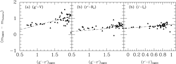
Figure 21. Photometry from GMOS-N (mag_Best from SExtractor) vs. photometry from Moran for galaxies in the MS0451.6−0305 field. Dashed lines: expected relations based on transformations from Jordi et al. (2006): (g' − V) = 0.565(g' − r') + 0.016; (r' − Rc) = 0.162(g' − r') + 0.110 and (r' − Rc) = 0.468(g' − r') − 0.305 for (g' − r') ⩽ 1.39 and (g' − r') > 1.39, respectively; (i' − Ic) = 0.232(r' − i') + 0.393.
Download figure:
Standard image High-resolution image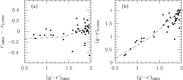
Figure 22. Photometry from GMOS-N vs. photometry from Ellingson et al. (1998) (CNOC) for the MS0451.6−0305 field. Dashed lines: expected relations based on transformations from Jørgensen (1994) and Jordi et al. (2006): (r' − rG) = 0.050(g' − r') − 0.170 and (r' − rG) = 0.299(g' − r') − 0.512 for (g' − r') ⩽ 1.39 and (g' − r') > 1.39, respectively; (gG − rG) = 1.005(r' − g') − 0.330 and (gG − rG) = 1.520(r' − g') − 0.995 for (g' − r') ⩽ 1.39 and (g' − r') > 1.39, respectively.
Download figure:
Standard image High-resolution image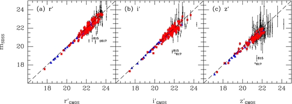
Figure 23. Photometry from GMOS-N (mag_Best from SExtractor) vs. photometry from SDSS DR7 for the RXJ1226.9+3332 field. Blue: stars included in the determination of the offsets; red: galaxies included in the offsets. Small black point: objects excluded due to large uncertainties or differences between GMOS and SDSS photometry. Dashed lines: one-to-one relations. The two galaxies ID = 617 and 815 deviate in all three comparisons. This is most likely due to bright close neighbors, which is affecting the SDSS photometry, while being taken better into account in the SExtractor processing of the GMOS-N photometry.
Download figure:
Standard image High-resolution imageTable 12. Comparison of GMOS-N and Other Ground-based Photometry
| Cluster | Comparison | Median Δa | rms | N | |
|---|---|---|---|---|---|
| MS0451.6−0305 | (g' − V) | −0.02a | 0.25 | 50 | Moran, Subaru data |
| MS0451.6−0305 | (r' − Rc) | 0.04a | 0.14 | 50 | Moran, Subaru data |
| MS0451.6−0305 | (i' − Ic) | −0.01a | 0.11 | 50 | Moran, Subaru data |
| MS0451.6−0305 | (r' − rG) | 0.017 b | 0.14 | 42 | CNOC |
| MS0451.6−0305 | (g' − r')c | −0.05b | 0.23 | 42 | CNOC |
| RXJ1226.9+3332 | (r' − r'SDSS) | 0.12d | 0.25 | 149 | SDSS, DR7 |
| RXJ1226.9+3332 | (i' − i'SDSS) | 0.06d | 0.26 | 155 | SDSS, DR7 |
| RXJ1226.9+3332 | (z' − z'SDSS) | 0.18d | 0.24 | 99 | SDSS, DR7 |
Notes. aComparison relative to expected relations shown in Figure 21. bComparison relative to expected relations shown in Figure 22. cOffset and scatter of (gG − rG) relative to the expected relation shown in Figure 22(b). dObjects with uncertainty larger than 0.5 mag on mSDSS and objects with |Δ| > 0.7 have been excluded.
Download table as: ASCIITypeset image
In summary, we conclude that our GMOS-N photometry is calibrated to an absolute accuracy of 0.05 mag. Tables 14 and 13 list the standard calibrated magnitudes and colors for the spectroscopic samples of MS0451.6−0305 and RXJ1226.6+3332, respectively. The photometry in these tables is not corrected for Galactic extinction.
Table 13. MS0451.6−0305: GMOS-N Photometric Data for the Spectroscopic Sample
| ID | R.A. (J2000) | Decl. (J2000)a | g'total | r'total | i'total | z'total | (g' − r') | (r' − i') | (i' − z') |
|---|---|---|---|---|---|---|---|---|---|
| 12 | 4 54 12.63 | −3 03 20.2 | 22.40 | 21.14 | 20.35 | 19.77 | 1.867 | 0.893 | 0.607 |
| 153 | 4 54 08.37 | −3 03 16.1 | 21.67 | 20.89 | 20.13 | 19.75 | 1.377 | 0.821 | 0.451 |
| 220 | 4 54 13.35 | −3 03 14.2 | 22.60 | 21.97 | 21.04 | 20.56 | 0.805 | 0.839 | 0.469 |
| 234 | 4 54 07.54 | −3 03 10.3 | 21.98 | 21.30 | 21.04 | 20.73 | 0.852 | 0.080 | 0.322 |
| 258 | 4 54 01.09 | −3 03 08.3 | 23.52 | 22.13 | 21.63 | 21.14 | 1.528 | 0.458 | 0.417 |
| 299 | 4 54 11.91 | −3 02 40.3 | 21.64 | 20.00 | 19.00 | 18.52 | 1.917 | 0.904 | 0.497 |
| 309 | 4 54 07.88 | −3 03 00.6 | 23.92 | 22.48 | 21.60 | 21.23 | 1.641 | 0.711 | 0.399 |
| 323 | 4 54 07.33 | −3 02 55.8 | 22.65 | 21.31 | 20.13 | 19.66 | 1.719 | 0.984 | 0.470 |
| 386 | 4 54 06.49 | −3 02 55.9 | 24.39 | 23.99 | 22.89 | 22.17 | 1.658 | 1.003 | 0.804 |
| 468 | 4 54 07.33 | −3 02 47.9 | 24.67 | 23.63 | 22.67 | 21.63 | 1.182 | 0.781 | 1.027 |
| 554 | 4 54 18.72 | −3 02 36.7 | 23.61 | 22.20 | 21.32 | 20.86 | 1.685 | 0.732 | 0.454 |
| 600 | 4 54 15.14 | −3 02 33.2 | 22.90 | 21.62 | 20.74 | 20.34 | 1.706 | 0.654 | 0.445 |
| 606 | 4 54 05.40 | −3 02 29.5 | 23.29 | 21.81 | 20.86 | 20.44 | 1.746 | 0.790 | 0.438 |
| 684 | 4 54 12.44 | −3 02 16.9 | 23.38 | 21.78 | 21.03 | 20.59 | 1.775 | 0.680 | 0.436 |
| 716 | 4 54 13.68 | −3 02 21.8 | 23.50 | 21.86 | 21.03 | 20.57 | 1.789 | 0.756 | 0.454 |
| 722 | 4 54 12.33 | −3 02 24.4 | 23.81 | 22.68 | 22.43 | 22.02 | 1.232 | 0.300 | 0.326 |
| 833 | 4 54 21.27 | −3 02 17.2 | 25.25 | 24.43 | 23.03 | 22.31 | 1.609 | 1.051 | 0.878 |
| 836 | 4 54 02.97 | −3 02 10.3 | 21.76 | 21.25 | 21.14 | 20.84 | 0.741 | −0.045 | 0.253 |
| 897 | 4 54 20.36 | −3 02 03.8 | 23.22 | 21.76 | 20.81 | 20.40 | 1.845 | 0.811 | 0.422 |
| 901 | 4 54 08.24 | −3 02 04.9 | 22.61 | 21.99 | 21.13 | 20.34 | 0.822 | 0.767 | 0.788 |
| 921 | 4 54 15.29 | −3 01 57.0 | 22.14 | 20.82 | 19.84 | 19.37 | 1.864 | 0.897 | 0.443 |
| 971 | 4 54 17.86 | −3 01 46.6 | 22.15 | 20.55 | 19.60 | 19.14 | 1.875 | 0.859 | 0.460 |
| 1002 | 4 54 17.22 | −3 01 56.6 | 23.08 | 21.58 | 20.81 | 20.43 | 1.794 | 0.794 | 0.392 |
| 1082 | 4 54 11.32 | −3 01 40.8 | 22.84 | 21.13 | 20.20 | 19.72 | 1.878 | 0.849 | 0.473 |
| 1156 | 4 54 04.37 | −3 01 41.6 | 22.24 | 21.18 | 20.51 | 20.04 | 1.384 | 0.688 | 0.487 |
| 1204 | 4 54 10.86 | −3 01 36.2 | 23.13 | 21.37 | 20.44 | 20.00 | 1.933 | 0.807 | 0.467 |
| 1331 | 4 54 16.78 | −3 01 30.7 | 22.76 | 21.37 | 20.77 | 20.43 | 1.672 | 0.502 | 0.351 |
| 1491 | 4 54 08.53 | −3 01 18.7 | 22.39 | 21.83 | 21.27 | 20.97 | 1.407 | 0.671 | 0.427 |
| 1497 | 4 54 12.47 | −3 01 07.7 | 22.16 | 20.86 | 20.07 | 19.75 | 1.859 | 0.752 | 0.441 |
| 1500 | 4 54 12.18 | −3 01 00.9 | 21.72 | 20.75 | 19.87 | 19.64 | 1.965 | 0.874 | 0.476 |
| 1507 | 4 54 12.44 | −3 01 16.6 | 23.11 | 21.61 | 20.64 | 20.20 | 1.927 | 0.840 | 0.467 |
| 1584 | 4 54 15.48 | −3 01 12.9 | 26.35 | 23.81 | 22.83 | 21.95 | 1.947 | 0.968 | 0.869 |
| 1594 | 4 54 14.80 | −3 01 05.6 | 22.62 | 21.14 | 20.15 | 19.69 | 1.948 | 0.839 | 0.483 |
| 1638 | 4 54 09.60 | −3 01 00.5 | 23.02 | 21.43 | 20.44 | 20.00 | 1.867 | 0.834 | 0.473 |
| 1720 | 4 54 10.84 | −3 00 51.6 | 21.26 | 20.00 | 19.00 | 18.81 | 1.698 | 0.890 | 0.436 |
| 1723 | 4 54 18.74 | −3 00 55.0 | 21.49 | 20.13 | 19.45 | 19.10 | 1.591 | 0.626 | 0.399 |
| 1753 | 4 54 10.40 | −3 00 46.7 | 21.84 | 20.63 | 19.77 | 19.58 | 1.582 | 0.677 | 0.450 |
| 1823 | 4 54 09.22 | −3 00 50.3 | 23.08 | 21.33 | 20.32 | 19.91 | 1.955 | 0.831 | 0.458 |
| 1904 | 4 54 05.71 | −3 00 40.4 | 23.04 | 21.59 | 20.71 | 20.18 | 1.872 | 0.822 | 0.495 |
| 1931 | 4 54 14.26 | −3 00 40.6 | 22.77 | 21.41 | 20.45 | 20.00 | 1.813 | 0.841 | 0.475 |
| 1952 | 4 54 14.47 | −3 00 32.0 | 22.49 | 21.15 | 20.13 | 19.69 | 1.900 | 0.855 | 0.486 |
| 2031 | 4 54 08.70 | −3 00 35.5 | 23.11 | 21.56 | 20.56 | 20.12 | 1.930 | 0.813 | 0.467 |
| 2032 | 4 54 01.85 | −3 00 29.4 | 21.76 | 21.24 | 20.94 | 20.95 | 0.709 | 0.121 | −0.012 |
| 2127 | 4 54 15.08 | −3 00 22.6 | 21.16 | 20.34 | 19.93 | 19.73 | 0.957 | 0.265 | 0.259 |
| 2166 | 4 54 04.49 | −3 00 13.9 | 21.39 | 20.54 | 20.05 | 19.70 | 1.152 | 0.497 | 0.424 |
| 2223 | 4 54 09.72 | −3 00 15.1 | 23.41 | 21.96 | 21.04 | 20.60 | 1.748 | 0.807 | 0.460 |
| 2230 | 4 54 14.35 | −3 00 17.9 | 25.12 | 23.07 | 21.99 | 21.25 | 2.219 | 1.112 | 0.868 |
| 2240 | 4 54 10.57 | −3 00 21.4 | 24.83 | 23.02 | 22.07 | 21.69 | 1.886 | 0.814 | 0.436 |
| 2491 | 4 54 14.70 | −2 59 07.2 | 23.83 | 22.92 | 21.94 | 21.17 | 1.198 | 0.905 | 0.750 |
| 2561 | 4 54 12.26 | −2 59 11.8 | 23.67 | 23.09 | 22.69 | 21.73 | 0.714 | 0.459 | 0.906 |
| 2563 | 4 54 14.13 | −2 59 29.4 | 22.34 | 20.73 | 19.85 | 19.38 | 1.844 | 0.813 | 0.442 |
| 2645 | 4 54 05.55 | −2 59 18.5 | 20.87 | 20.10 | 19.66 | 19.37 | 1.088 | 0.517 | 0.389 |
| 2657 | 4 54 03.88 | −2 59 18.4 | 21.50 | 20.61 | 20.04 | 19.73 | 1.101 | 0.571 | 0.359 |
| 2689 | 4 54 01.52 | −2 59 24.0 | 22.85 | 21.60 | 20.72 | 20.32 | 1.677 | 0.777 | 0.401 |
| 2788 | 4 54 10.52 | −2 59 32.2 | 23.36 | 21.72 | 20.84 | 20.28 | 1.912 | 0.798 | 0.516 |
| 2913 | 4 54 04.89 | −3 00 01.3 | 22.50 | 21.04 | 20.08 | 19.60 | 1.909 | 0.832 | 0.481 |
| 2945 | 4 54 07.01 | −2 59 45.0 | 23.70 | 21.80 | 20.91 | 20.44 | 1.953 | 0.746 | 0.472 |
| 3005 | 4 54 16.65 | −2 59 46.0 | 25.34 | 23.16 | 21.95 | 21.03 | 2.282 | 1.074 | 0.934 |
| 3124 | 4 54 12.07 | −3 00 01.1 | 22.87 | 21.50 | 20.64 | 20.14 | 1.844 | 0.806 | 0.468 |
| 3260 | 4 54 07.57 | −3 00 08.2 | 23.96 | 22.52 | 21.57 | 21.13 | 1.827 | 0.784 | 0.473 |
| 3521 | 4 54 20.99 | −2 58 30.7 | 22.60 | 20.92 | 20.18 | 19.77 | 1.657 | 0.597 | 0.436 |
| 3610 | 4 54 15.02 | −2 58 17.0 | 22.50 | 21.61 | 21.21 | 20.92 | 0.988 | 0.272 | 0.292 |
| 3625 | 4 54 16.85 | −2 58 18.4 | 25.63 | 23.04 | 22.05 | 21.02 | 2.403 | 1.023 | 1.035 |
| 3635 | 4 54 13.07 | −2 58 24.3 | 25.30 | 23.81 | 22.65 | 22.01 | 1.930 | 1.164 | 0.712 |
| 3697 | 4 54 07.07 | −2 58 37.5 | 22.93 | 22.42 | 22.00 | 21.84 | 0.966 | 0.311 | 0.206 |
| 3724 | 4 54 06.85 | −2 58 59.3 | 23.14 | 21.98 | 21.09 | 20.68 | 1.811 | 0.758 | 0.459 |
| 3749 | 4 54 06.86 | −2 59 03.8 | 22.99 | 21.91 | 21.06 | 20.69 | 1.768 | 0.755 | 0.444 |
| 3792 | 4 54 02.74 | −2 58 40.4 | 23.84 | 23.26 | 22.30 | 21.89 | 0.825 | 0.755 | 0.472 |
| 3857 | 4 54 09.85 | −2 58 44.7 | 23.74 | 22.04 | 21.22 | 20.70 | 1.860 | 0.732 | 0.465 |
| 3906 | 4 54 10.38 | −2 58 51.4 | 24.66 | 23.62 | 22.93 | 22.01 | 1.193 | 0.539 | 0.919 |
Notes. Units of right ascension are hours, minutes, and seconds, and units of declination are degrees, arcminutes, and arcseconds.
aPositions are consistent with USNO (Monet et al. 1998), with an rms scatter of ≈07.
Download table as: ASCIITypeset image
Table 14. RXJ1226.9+3332: GMOS-N Photometric Data for the Spectroscopic Sample
| ID | R.A. (J2000) | Decl. (J2000)a | r'total | i'total | z'total | (r' − i') | (i' − z') |
|---|---|---|---|---|---|---|---|
| 18 | 12 27 06.81 | 33 35 29.7 | 23.08 | 21.86 | 21.35 | 1.160 | 0.676 |
| 38 | 12 27 05.65 | 33 35 28.6 | 23.61 | 22.43 | 21.77 | 1.191 | 0.729 |
| 53 | 12 27 06.23 | 33 35 22.4 | 22.48 | 22.47 | 22.20 | −0.107 | 0.357 |
| 55 | 12 26 53.16 | 33 35 13.7 | 23.09 | 21.80 | 21.16 | 1.271 | 0.707 |
| 56 | 12 27 08.86 | 33 35 19.9 | 23.07 | 21.79 | 21.66 | 1.166 | 0.691 |
| 91 | 12 27 06.64 | 33 35 08.2 | 24.37 | 23.49 | 23.18 | 0.696 | 0.287 |
| 104 | 12 26 59.78 | 33 35 02.1 | 23.68 | 22.50 | 21.79 | 1.207 | 0.725 |
| 122 | 12 27 01.32 | 33 34 56.3 | 23.96 | 22.44 | 22.10 | 1.255 | 0.664 |
| 132 | 12 26 47.77 | 33 34 48.3 | 22.16 | 21.23 | 20.95 | 1.203 | 0.458 |
| 138 | 12 27 00.63 | 33 34 46.9 | 22.31 | 21.03 | 20.68 | 1.219 | 0.466 |
| 153 | 12 26 52.68 | 33 34 46.3 | 22.37 | 22.11 | 21.98 | 0.242 | 0.148 |
| 154 | 12 26 47.80 | 33 34 44.6 | 23.45 | 22.37 | 21.79 | 1.099 | 0.403 |
| 178 | 12 26 48.35 | 33 34 40.2 | 22.23 | 21.95 | 21.96 | 0.271 | 0.043 |
| 185 | 12 26 53.32 | 33 34 36.2 | 22.80 | 21.51 | 21.09 | 1.329 | 0.559 |
| 203 | 12 26 59.35 | 33 34 19.9 | 21.77 | 21.06 | 21.02 | 0.783 | 0.246 |
| 220 | 12 26 55.16 | 33 34 25.5 | 23.22 | 22.02 | 21.66 | 1.218 | 0.499 |
| 229 | 12 27 07.35 | 33 34 24.3 | 23.57 | 22.28 | 21.87 | 1.229 | 0.704 |
| 245 | 12 27 07.42 | 33 34 19.7 | 23.45 | 22.31 | 21.75 | 1.181 | 0.751 |
| 247 | 12 26 51.34 | 33 34 14.9 | 20.23 | 19.73 | 19.47 | 0.480 | 0.381 |
| 249 | 12 26 52.08 | 33 34 12.5 | 20.81 | 20.37 | 20.22 | 0.417 | 0.237 |
| 293 | 12 27 05.85 | 33 34 05.2 | 23.00 | 21.77 | 21.27 | 1.266 | 0.725 |
| 295 | 12 27 02.18 | 33 34 06.4 | 22.93 | 21.67 | 21.40 | 1.153 | 0.651 |
| 297 | 12 26 49.78 | 33 34 10.4 | 24.22 | 23.63 | 23.10 | 0.444 | 0.695 |
| 309 | 12 27 04.45 | 33 34 06.8 | 24.44 | 23.23 | 22.46 | 1.166 | 0.743 |
| 310 | 12 26 53.25 | 33 34 05.7 | 24.11 | 22.84 | 22.21 | 1.237 | 0.716 |
| 316 | 12 26 59.58 | 33 34 04.3 | 23.51 | 22.96 | 22.59 | 0.616 | 0.485 |
| 329 | 12 26 54.54 | 33 33 56.6 | 21.51 | 21.04 | 21.11 | 0.507 | 0.181 |
| 333 | 12 27 00.44 | 33 33 59.2 | 23.92 | 23.12 | 23.19 | 0.729 | 0.140 |
| 347 | 12 27 04.39 | 33 33 52.6 | 21.30 | 20.89 | 20.54 | 0.334 | 0.422 |
| 349 | 12 27 01.33 | 33 33 53.4 | 22.18 | 21.27 | 20.89 | 0.840 | 0.478 |
| 359 | 12 26 54.38 | 33 33 51.0 | 22.46 | 21.67 | 21.54 | 0.777 | 0.297 |
| 374 | 12 27 02.07 | 33 33 43.6 | 21.99 | 21.56 | 21.55 | 0.402 | 0.308 |
| 386 | 12 26 54.48 | 33 33 40.7 | 23.05 | 22.18 | 21.91 | 0.815 | 0.420 |
| 408 | 12 26 54.25 | 33 33 34.8 | 23.54 | 22.37 | 21.88 | 1.132 | 0.693 |
| 423 | 12 26 53.15 | 33 33 31.4 | 23.53 | 22.23 | 21.64 | 1.245 | 0.727 |
| 441 | 12 26 53.86 | 33 33 28.9 | 24.37 | 23.08 | 22.77 | 1.253 | 0.718 |
| 446 | 12 27 06.76 | 33 33 27.1 | 23.45 | 22.14 | 21.66 | 1.209 | 0.662 |
| 452 | 12 26 53.99 | 33 33 23.1 | 23.42 | 22.31 | 21.98 | 1.194 | 0.614 |
| 462 | 12 26 52.47 | 33 33 24.2 | 23.75 | 22.67 | 21.92 | 1.182 | 0.772 |
| 470 | 12 26 54.90 | 33 33 24.5 | 24.97 | 23.67 | 23.10 | 1.231 | 0.714 |
| 491 | 12 26 57.55 | 33 33 14.0 | 23.35 | 21.95 | 21.46 | 1.326 | 0.698 |
| 499 | 12 27 07.72 | 33 33 14.3 | 24.12 | 23.02 | 22.39 | 1.147 | 0.598 |
| 500 | 12 26 53.55 | 33 33 10.1 | 22.09 | 21.37 | 21.10 | 0.735 | 0.445 |
| 512 | 12 26 55.67 | 33 33 13.1 | 24.91 | 23.55 | 22.91 | 1.303 | 0.744 |
| 523 | 12 26 57.18 | 33 33 05.1 | 23.26 | 21.94 | 21.64 | 1.253 | 0.738 |
| 527 | 12 27 07.77 | 33 33 11.1 | 24.67 | 24.40 | 23.56 | 0.252 | 0.697 |
| 528 | 12 27 04.49 | 33 33 07.8 | 22.96 | 21.90 | 21.24 | 1.092 | 0.690 |
| 529 | 12 27 01.38 | 33 33 04.8 | 22.92 | 21.55 | 21.03 | 1.288 | 0.734 |
| 534 | 12 26 56.83 | 33 33 06.3 | 23.97 | 22.47 | 21.90 | 1.293 | 0.728 |
| 547 | 12 26 54.23 | 33 32 53.6 | 23.26 | 22.20 | 21.82 | 1.085 | 0.577 |
| 557 | 12 27 07.72 | 33 32 56.1 | 23.50 | 22.32 | 21.84 | 1.222 | 0.740 |
| 563 | 12 26 58.29 | 33 32 49.0 | 21.17 | 19.86 | 18.15 | 1.352 | 0.719 |
| 572 | 12 27 02.65 | 33 32 57.5 | 22.88 | 22.11 | 21.98 | 0.704 | 0.341 |
| 592 | 12 26 50.22 | 33 32 53.3 | 22.31 | 22.56 | 22.05 | −0.282 | 0.513 |
| 593 | 12 26 57.08 | 33 32 53.5 | 24.38 | 22.80 | 22.40 | 1.359 | 0.712 |
| 602 | 12 26 53.01 | 33 32 49.9 | 22.96 | 21.80 | 21.23 | 1.194 | 0.610 |
| 608 | 12 26 50.63 | 33 32 46.5 | 22.95 | 21.87 | 21.39 | 1.189 | 0.711 |
| 630 | 12 26 57.35 | 33 32 46.9 | 24.82 | 23.34 | 23.08 | 1.318 | 0.725 |
| 641 | 12 26 59.28 | 33 32 40.9 | 23.37 | 21.95 | 21.97 | 1.298 | 0.683 |
| 647 | 12 27 00.00 | 33 32 40.9 | 23.35 | 22.15 | 22.46 | 1.069 | 0.655 |
| 648 | 12 26 50.41 | 33 32 41.7 | 23.41 | 22.11 | 21.56 | 1.296 | 0.694 |
| 649 | 12 26 56.33 | 33 32 41.2 | 24.38 | 23.06 | 22.48 | 1.232 | 0.728 |
| 650 | 12 27 10.57 | 33 32 41.9 | 23.99 | 22.87 | 22.32 | 1.133 | 0.709 |
| 656 | 12 26 56.72 | 33 32 40.7 | 23.47 | 22.20 | 21.73 | 1.243 | 0.727 |
| 675 | 12 26 54.68 | 33 32 35.6 | 23.63 | 22.52 | 22.13 | 1.259 | 0.709 |
| 685 | 12 26 54.80 | 33 32 34.4 | 24.05 | 23.21 | 22.71 | 0.814 | 0.644 |
| 689 | 12 26 55.30 | 33 32 32.8 | 23.77 | 22.54 | 22.07 | 1.248 | 0.722 |
| 703 | 12 26 56.12 | 33 32 23.4 | 22.22 | 20.83 | 20.44 | 1.265 | 0.734 |
| 709 | 12 26 57.13 | 33 32 27.8 | 23.52 | 22.22 | 21.81 | 1.254 | 0.693 |
| 711 | 12 27 00.52 | 33 32 30.1 | 24.94 | 23.75 | 23.29 | 1.000 | 0.500 |
| 739 | 12 27 04.09 | 33 30 56.1 | 23.89 | 22.66 | 21.80 | 1.251 | 0.799 |
| 754 | 12 26 58.54 | 33 31 03.1 | 21.92 | 21.83 | 21.67 | −0.016 | 0.231 |
| 757 | 12 27 04.65 | 33 31 01.2 | 24.11 | 23.03 | 22.35 | 1.101 | 0.755 |
| 760 | 12 27 03.83 | 33 31 01.5 | 23.52 | 22.16 | 21.53 | 1.294 | 0.701 |
| 781 | 12 26 46.73 | 33 31 03.8 | 23.60 | 22.35 | 21.82 | 1.249 | 0.505 |
| 798b | 12 26 56.11 | 33 31 09.5 | 25.80 | 24.95 | 24.54 | 0.919 | 0.725 |
| 801 | 12 27 07.23 | 33 31 15.9 | 23.04 | 21.95 | 21.44 | 1.140 | 0.718 |
| 805 | 12 27 04.35 | 33 31 21.6 | 22.85 | 22.02 | 21.79 | 0.798 | 0.483 |
| 824 | 12 27 01.58 | 33 31 18.4 | 21.52 | 20.83 | 20.76 | 0.632 | 0.360 |
| 841 | 12 27 04.49 | 33 31 32.9 | 21.75 | 21.45 | 21.26 | 0.296 | 0.348 |
| 861 | 12 27 04.90 | 33 31 32.5 | 21.99 | 21.36 | 21.13 | 0.564 | 0.424 |
| 863 | 12 27 00.87 | 33 31 27.1 | 22.99 | 21.79 | 21.55 | 1.146 | 0.505 |
| 872 | 12 26 58.08 | 33 31 34.6 | 23.12 | 22.48 | 22.20 | 0.340 | 0.033 |
| 883 | 12 26 56.32 | 33 31 37.2 | 24.59 | 23.34 | 22.78 | 1.210 | 0.718 |
| 899 | 12 26 45.63 | 33 31 40.7 | 23.54 | 22.41 | 20.83 | 1.177 | 0.719 |
| 907 | 12 27 05.19 | 33 31 42.8 | 23.01 | 22.15 | 21.93 | 1.002 | 0.484 |
| 928 | 12 27 09.15 | 33 31 47.1 | 20.76 | 20.19 | 19.82 | 0.578 | 0.544 |
| 933 | 12 26 52.98 | 33 31 46.9 | 24.16 | 23.05 | 22.59 | 1.167 | 0.673 |
| 934 | 12 26 53.53 | 33 31 50.2 | 21.29 | 20.88 | 21.03 | 0.428 | 0.250 |
| 960 | 12 27 04.98 | 33 31 56.2 | 22.37 | 21.42 | 21.30 | 0.891 | 0.363 |
| 968 | 12 26 55.83 | 33 31 53.4 | 24.06 | 22.71 | 22.07 | 1.240 | 0.737 |
| 982 | 12 27 03.02 | 33 31 57.3 | 19.72 | 19.39 | 19.38 | 0.154 | 0.050 |
| 995 | 12 26 46.13 | 33 32 01.5 | 23.03 | 21.89 | 21.28 | 1.268 | 0.664 |
| 996 | 12 26 55.64 | 33 32 13.1 | 21.92 | 20.71 | 19.61 | 1.260 | 0.687 |
| 999 | 12 26 51.27 | 33 32 05.2 | 24.27 | 22.97 | 22.75 | 1.320 | 0.603 |
| 1001 | 12 26 59.24 | 33 32 12.6 | 21.81 | 21.54 | 21.47 | 0.292 | 0.154 |
| 1005 | 12 26 54.82 | 33 32 21.8 | 23.12 | 22.22 | 22.14 | 0.801 | 0.311 |
| 1022 | 12 27 08.20 | 33 32 07.5 | 24.27 | 23.96 | 24.45 | 0.524 | −0.094 |
| 1025 | 12 26 56.57 | 33 32 19.7 | 23.66 | 22.67 | 22.31 | 1.192 | 0.666 |
| 1027 | 12 27 03.68 | 33 32 10.5 | 23.03 | 22.34 | 21.77 | 0.707 | 0.525 |
| 1029 | 12 27 06.01 | 33 32 12.0 | 23.16 | 22.64 | 22.46 | 0.505 | 0.431 |
| 1042 | 12 26 53.54 | 33 32 19.3 | 24.23 | 22.98 | 22.33 | 1.223 | 0.615 |
| 1047 | 12 26 56.08 | 33 32 15.7 | 23.25 | 21.92 | 21.47 | 1.252 | 0.676 |
| 1057 | 12 27 05.52 | 33 30 43.9 | 23.98 | 23.51 | 23.18 | 0.444 | 0.651 |
| 1080 | 12 27 01.74 | 33 30 25.3 | 22.83 | 22.22 | 22.72 | 0.434 | 0.058 |
| 1083 | 12 26 49.64 | 33 30 19.4 | 22.18 | 21.80 | 21.81 | 0.384 | 0.127 |
| 1091 | 12 27 08.23 | 33 32 13.1 | 23.64 | 22.66 | 22.10 | 0.934 | 0.717 |
| 1103 | 12 27 02.61 | 33 30 13.7 | 23.89 | 23.12 | 22.90 | 0.738 | 0.328 |
| 1157 | 12 27 03.56 | 33 30 14.2 | 24.08 | 23.33 | 22.75 | 0.798 | 0.543 |
| 1164 | 12 26 55.69 | 33 30 37.9 | 23.98 | 22.82 | 22.22 | 1.172 | 0.700 |
| 1170 | 12 26 49.39 | 33 30 31.4 | 23.26 | 21.99 | 21.33 | 1.258 | 0.703 |
| 1175 | 12 26 57.81 | 33 30 37.8 | 23.32 | 22.12 | 21.58 | 1.207 | 0.692 |
| 1182 | 12 26 53.88 | 33 30 44.9 | 24.59 | 23.87 | 23.30 | 0.709 | 0.474 |
| 1196 | 12 27 01.79 | 33 30 22.2 | 24.53 | 23.12 | 23.01 | 1.444 | 0.559 |
| 1199 | 12 27 08.57 | 33 30 48.2 | 23.86 | 22.75 | 22.12 | 1.075 | 0.773 |
| 1251 | 12 26 56.33 | 33 32 41.8 | 24.38 | 23.06 | 22.48 | 1.232 | 0.728 |
| 1252 | 12 27 03.15 | 33 31 55.4 | 23.17 | 21.77 | 21.26 | 1.281 | 0.552 |
| 1253 | 12 27 07.72 | 33 32 54.1 | 23.72 | 22.81 | 22.42 | 0.955 | 0.648 |
| 1254b | 12 26 56.11 | 33 31 09.5 | 23.41 | 22.56 | 22.16 | 0.919 | 0.725 |
Notes. Units of right ascension are hours, minutes, and seconds and units of declination are degrees, arcminutes, and arcseconds.
aPositions are consistent with USNO (Monet et al. 1998), with an rms scatter of ≈07.
bID = 798 and 1254 are listed at the same position as the galaxies are superimposed, as seen by two overlapping spectra in the slit.
A.2. Photometry from HST/ACS: Calibration and External Comparison
Total magnitudes, effective radii, and mean surface brightnesses for the spectroscopic sample in MS0451.6−0305 were derived using the fitting program GALFIT (Peng et al. 2002) and the techniques established for our project and described in detail in Chiboucas et al. (2009). Table 15 lists the resulting parameters for the fit with the r1/4 profile and with a Sérsic (1968) profile. The magnitudes are on the AB system, using a zero point for F814W of 25.937 (Sirianni et al. 2005). The photometry has not been corrected for Galactic extinction.
Table 15. MS0451.6−0305: Photometric Parameters from HST/ACS Data in F814W
| ID | mtot, dev | log re, dev | 〈μ〉e, dev | mtot, ser | log re, ser | 〈μ〉e, ser | nser | P.A. |  |
|---|---|---|---|---|---|---|---|---|---|
| (1) | (2) | (3) | (4) | (5) | (6) | (7) | (8) | (9) | (10) |
| 12 | 19.53 | 0.299 | 23.02 | 19.70 | 0.135 | 22.38 | 2.32 | −53.1 | 0.72 |
| 153 | 20.19 | −0.275 | 20.81 | 20.19 | −0.275 | 20.81 | 4.00 | 9.1 | 0.41 |
| 220 | 20.20 | 0.188 | 23.14 | 20.64 | −0.148 | 21.90 | 1.41 | 40.9 | 0.12 |
| 234 | 20.57 | −0.190 | 21.61 | 20.94 | −0.470 | 20.58 | 1.40 | 71.3 | 0.34 |
| 258 | 20.82 | −0.185 | 21.89 | 21.20 | −0.465 | 20.87 | 1.23 | 7.8 | 0.49 |
| 299 | 18.54 | 0.151 | 21.30 | 18.56 | 0.136 | 21.24 | 3.88 | 52.9 | 0.12 |
| 309 | 21.17 | −0.254 | 21.90 | 21.21 | −0.286 | 21.78 | 3.70 | −14.5 | 0.19 |
| 323 | 19.94 | −0.370 | 20.09 | 19.77 | −0.230 | 20.62 | 5.61 | 74.3 | 0.26 |
| 386 | 22.27 | −0.508 | 21.73 | 22.33 | −0.557 | 21.55 | 3.50 | 27.1 | 0.14 |
| 468 | 21.82 | −0.220 | 22.72 | 22.03 | −0.384 | 22.11 | 2.38 | 42.0 | 0.23 |
| 554 | 20.81 | −0.383 | 20.89 | 20.96 | −0.497 | 20.47 | 2.64 | −10.2 | 0.10 |
| 600 | 21.13 | −0.446 | 20.89 | 21.04 | −0.376 | 21.15 | 4.59 | 53.8 | 0.26 |
| 606 | 20.59 | −0.664 | 19.26 | 20.53 | −0.616 | 19.44 | 4.86 | −36.6 | 0.59 |
| 684 | 20.49 | −0.191 | 21.53 | 20.65 | −0.311 | 21.09 | 2.80 | −26.0 | 0.34 |
| 716 | 20.55 | −0.102 | 22.03 | 20.71 | −0.227 | 21.57 | 2.87 | −84.7 | 0.24 |
| 722 | 21.41 | 0.086 | 23.83 | 22.08 | −0.407 | 22.04 | 0.60 | −24.4 | 0.40 |
| 833 | 22.74 | −0.608 | 21.70 | 22.74 | −0.602 | 21.72 | 4.14 | −1.9 | 0.15 |
| 836 | 20.45 | 0.149 | 23.19 | 21.13 | −0.324 | 21.50 | 0.82 | 43.0 | 0.53 |
| 897 | 20.48 | −0.526 | 19.84 | 20.52 | −0.559 | 19.72 | 3.49 | −17.2 | 0.72 |
| 901 | 20.94 | −0.767 | 19.10 | 20.60 | −0.458 | 20.31 | 8.85 | 63.6 | 0.16 |
| 921 | 19.48 | −0.143 | 20.77 | 19.53 | −0.177 | 20.64 | 3.68 | 69.1 | 0.20 |
| 971 | 19.01 | 0.137 | 21.69 | 19.12 | 0.052 | 21.37 | 3.42 | 12.3 | 0.21 |
| 1002 | 20.10 | 0.146 | 22.82 | 20.31 | −0.005 | 22.28 | 2.89 | −54.1 | 0.28 |
| 1082 | 19.79 | −0.224 | 20.67 | 19.76 | −0.200 | 20.76 | 4.24 | 0.2 | 0.20 |
| 1156 | 20.28 | −0.173 | 21.41 | 20.46 | −0.305 | 20.92 | 2.73 | −4.8 | 0.61 |
| 1204 | 20.08 | −0.308 | 20.53 | 20.06 | −0.289 | 20.60 | 4.20 | 13.6 | 0.34 |
| 1331 | 20.38 | −0.198 | 21.39 | 20.52 | −0.317 | 20.93 | 2.54 | 53.5 | 0.65 |
| 1491 | 21.46 | −0.836 | 19.27 | 21.54 | −0.893 | 19.07 | 2.84 | 82.7 | 0.54 |
| 1497 | 19.95 | −0.429 | 19.80 | 19.87 | −0.373 | 20.00 | 4.69 | −8.2 | 0.45 |
| 1500 | 19.60 | 0.018 | 21.69 | 19.88 | −0.190 | 20.93 | 2.50 | −75.5 | 0.09 |
| 1507 | 20.39 | −0.551 | 19.63 | 20.40 | −0.556 | 19.61 | 3.93 | 13.1 | 0.35 |
| 1584 | 22.48 | −0.582 | 21.56 | 22.47 | −0.575 | 21.59 | 4.08 | 19.3 | 0.42 |
| 1594 | 19.87 | −0.237 | 20.68 | 19.75 | −0.141 | 21.05 | 4.92 | −34.9 | 0.19 |
| 1638 | 20.12 | −0.172 | 21.26 | 19.95 | −0.022 | 21.83 | 5.40 | 40.8 | 0.07 |
| 1720 | 18.47 | 0.367 | 22.29 | 18.12 | 0.588 | 23.06 | 5.28 | −70.1 | 0.30 |
| 1723 | 18.98 | 0.017 | 21.06 | 19.27 | −0.194 | 20.29 | 1.51 | 76.1 | 0.80 |
| 1753 | 20.16 | −0.298 | 20.66 | 19.83 | −0.020 | 21.73 | 6.37 | −61.7 | 0.30 |
| 1823 | 19.98 | −0.353 | 20.21 | 19.89 | −0.278 | 20.50 | 4.84 | −70.2 | 0.29 |
| 1904 | 20.35 | −0.408 | 20.30 | 20.32 | −0.389 | 20.37 | 4.22 | −38.8 | 0.29 |
| 1931 | 20.11 | −0.266 | 20.78 | 20.20 | −0.333 | 20.53 | 3.31 | −57.1 | 0.31 |
| 1952 | 19.88 | −0.247 | 20.64 | 19.89 | −0.255 | 20.61 | 3.82 | −41.6 | 0.16 |
| 2031 | 20.41 | −0.553 | 19.64 | 20.38 | −0.527 | 19.74 | 4.34 | −70.5 | 0.51 |
| 2032 | 21.01 | −0.675 | 19.63 | 21.03 | −0.778 | 19.13 | 1.10 | 60.3 | 0.16 |
| 2127 | 19.36 | 0.244 | 22.57 | 19.91 | −0.162 | 21.09 | 0.89 | −71.2 | 0.51 |
| 2166 | 20.07 | −0.015 | 21.99 | 20.04 | −0.022 | 21.92 | 1.11 | −67.1 | 0.41 |
| 2223 | 20.89 | −0.401 | 20.88 | 20.71 | −0.387 | 20.77 | 2.77 | 10.3 | 0.34 |
| 2230 | 21.60 | −0.344 | 21.88 | 21.54 | −0.289 | 22.09 | 4.51 | −6.2 | 0.12 |
| 2240 | 21.60 | −0.581 | 20.70 | 21.75 | −0.680 | 20.34 | 2.40 | 85.9 | 0.62 |
| 2491 | 21.43 | −0.316 | 21.85 | 21.43 | −0.354 | 21.66 | 2.54 | −58.2 | 0.15 |
| 2561 | 22.17 | −0.379 | 22.27 | 22.06 | −0.282 | 22.65 | 4.96 | −85.5 | 0.46 |
| 2563 | 19.40 | 0.262 | 22.70 | 19.37 | 0.267 | 22.70 | 3.86 | −28.9 | 0.12 |
| 2645 | 19.01 | 0.335 | 22.68 | 19.43 | 0.020 | 21.52 | 1.45 | 77.5 | 0.47 |
| 2657 | 19.25 | 0.419 | 23.34 | 19.91 | −0.058 | 21.62 | 0.78 | −48.7 | 0.13 |
| 2689 | 20.39 | −0.598 | 19.39 | 20.41 | −0.616 | 19.33 | 3.71 | −47.4 | 0.68 |
| 2788 | 20.57 | −0.309 | 21.01 | 20.40 | −0.275 | 21.02 | 2.77 | 74.5 | 0.13 |
| 2913 | 19.79 | −0.315 | 20.21 | 19.78 | −0.305 | 20.26 | 4.16 | −2.1 | 0.19 |
| 2945 | 20.58 | −0.445 | 20.36 | 20.67 | −0.518 | 20.08 | 2.73 | 28.2 | 0.38 |
| 3005 | 21.18 | −0.192 | 22.22 | 21.38 | −0.348 | 21.64 | 2.69 | −32.3 | 0.21 |
| 3124 | 20.07 | −0.114 | 21.50 | 20.23 | −0.234 | 21.05 | 2.90 | −28.3 | 0.58 |
| 3260 | 21.27 | −0.752 | 19.50 | 21.17 | −0.679 | 19.77 | 5.43 | 36.4 | 0.69 |
| 3521 | 19.75 | 0.019 | 21.84 | 19.95 | −0.132 | 21.28 | 2.68 | 38.8 | 0.25 |
| 3610 | 20.54 | 0.159 | 23.33 | 21.22 | −0.362 | 21.41 | 0.39 | −57.7 | 0.80 |
| 3625 | 21.54 | −0.388 | 21.60 | 21.36 | −0.238 | 22.17 | 5.36 | −62.9 | 0.13 |
| 3635 | 22.34 | −0.430 | 22.18 | 22.13 | −0.434 | 21.95 | 3.75 | 69.4 | 0.73 |
| 3697 | 22.16 | −0.632 | 20.99 | 22.47 | −0.846 | 20.24 | 1.32 | 48.3 | 0.15 |
| 3724 | 20.93 | −0.492 | 20.47 | 20.87 | −0.442 | 20.66 | 4.59 | −50.8 | 0.15 |
| 3749 | 20.90 | −0.283 | 21.48 | 20.77 | −0.180 | 21.87 | 5.06 | 82.4 | 0.18 |
| 3792 | 21.39 | 0.161 | 24.18 | 22.05 | −0.344 | 22.32 | 0.50 | 18.5 | 0.48 |
| 3857 | 20.84 | −0.408 | 20.79 | 20.87 | −0.436 | 20.69 | 3.68 | −34.4 | 0.46 |
| 3906 | 22.51 | −0.375 | 22.63 | 22.57 | −0.420 | 22.46 | 3.61 | 81.1 | 0.14 |
Notes. Column 1: galaxy ID; Column 2: total magnitude from fit with r1/4 profile; Column 3: logarithm of the effective radius in arcseconds from fit with r1/4 profile; Column 4: mean surface brightness in mag arcsec−2 within the effective radius, from fit with r1/4 profile; Columns 5–7: total magnitude, logarithm of the effective radius, and the mean surface brightness, from fit with a Sérsic profile; Column 8: Sérsic index; Column 9: position angle of the major axis measured from north through east; Column 10: ellipticity.
Download table as: ASCIITypeset image
We have compared our GALFIT results with data from S. Moran (2011, private communication) who also used GALFIT to process the HST/ACS data, but with a different PSF model. Figure 24 and Table 16 summarize the comparison. As the errors in the total magnitude and the effective radii are correlated (e.g., Jørgensen et al. 1995a) we also show the comparison as the difference in magnitude versus the difference in effective radius. The four galaxies deviating from the correlation are labeled. Two of these (ID = 2166 and 2645) are spirals or irregulars possibly causing the large difference between the two sets of data. The other two (ID = 1720 and 2563) have close neighbors. The detailed handling of these when running GALFIT is likely to affect the resulting parameters and could be the cause of the large differences between the two sets of data. We also note that for ID = 2563 the GALFIT magnitude from Moran deviates with more than 1 mag from the Subaru ground based data made available at Moran's Web site http://www.astro.caltech.edu/~smm/clusters/. The photometry from Moran is on the Vega system with an F814W zero point of 25.501. Thus, the expected offset is 0.436 mag. Excluding the four outliers marked in the figure, we determine the offset between the two data sets by fitting a line to the data shown in Figure 24(c). The intersect between the fit and the y-axis gives an offset of 0.401 mag. This method of determining the offset between the magnitudes is more robust than a direct comparison as it eliminates the effect of the correlated errors. Thus, our magnitudes are 0.035 mag brighter than those determined by Moran. This difference is most likely due to difference in the PSFs used in our work and that by Moran; see Chiboucas et al. (2009).

Figure 24. Photometry from HST/ACS F814W vs. similar photometry from S. Moran (2011, private communication) for the MS0451.6−0306 field. The dashed line in (b) marks the expected offset between our AB magnitudes and the Vega magnitudes from Moran. (c) Difference in magnitudes vs. difference in the logarithm to the semi-major axes. The errors on these parameters are correlated. From the linear fit (solid line) we determine a magnitude offset between the two data sets of 0.401 mag; see the text for details.
Download figure:
Standard image High-resolution imageTable 16. Comparison of HST/ACS Photometry for MS0451.6−0305
| Comparison | Median Δ | rms | N |
|---|---|---|---|
| (log ae − log ae, Moran) | −0.06 | 0.16 | 23 |
| (F814WAB − F814WVega, Moran) | 0.48 | 0.19 | 23 |
| (F814WAB − F814WVega, Moran)a | 0.40 | 0.02 | 23 |
Notes. aMagnitude difference determined from the intersect of fit shown in Figure 24.
Download table as: ASCIITypeset image
For the purpose of calibrating the HST/ACS photometry to the rest frame, we have chosen first to calibrate the F775W (RXJ0152.7−1357) and F814W (MS0451.6−0305 and RXJ1226.9+3332) AB magnitudes to i' magnitudes. We use the synthetic transformations from Sirianni et al. (2005) listed in their Table 3 together with transformations from Jordi et al. (2006) in order to transform from Ic to i' (Ic = i' − 0.245(r' − i') − 0.387). While one could argue that a more direct calibration would be preferable, we judge that our method do not add significantly to the systematic effects on the data as these are dominated by the underlying assumptions of the spectral energy distributions. When applying the transformation, we use the (r' − i') colors from our GMOS photometry.
Figure 25 and Table 17 summarize the comparison of our GMOS-N photometry (derived with SExtractor) and the HST/ACS photometry (derived with GALFIT) calibrated to the i' band. The expected offset between the magnitudes is 0.06 mag, due to the systematically missed flux in the best magnitudes from SExtractor (Bertin & Arnouts 1996). For RXJ0152.7−1357 and RXJ1226.9+3332 the magnitudes agree within the uncertainties, while the median offset for MS0451.6−0305 deviates with 0.08 mag from the expectations, roughly a 3σ difference given the scatter in the comparison. We take this as the upper limit on systematic errors affecting the photometry.
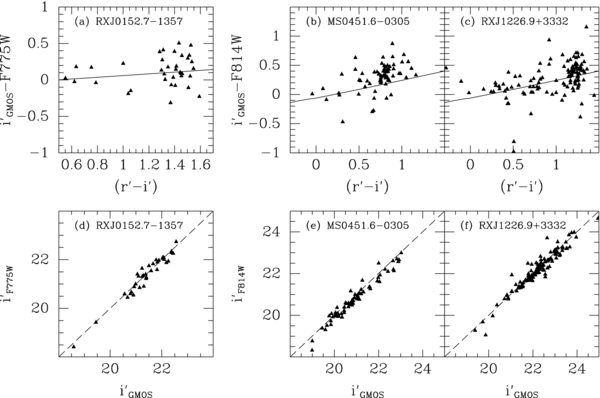
Figure 25. Top panels: differences between total magnitudes from the Sérsic fits to the HST/ACS images and the total magnitudes mag_Best from the GMOS-N i'-band images. Solid lines show the expected relations; see the text. Bottom panels: HST/ACS total magnitudes calibrated to the i' band vs. the total magnitudes mag_Best from the GMOS-N i'-band images. Dashed lines show the one-to-one relations.
Download figure:
Standard image High-resolution imageTable 17. Comparison of GMOS-N and HST/ACS Photometry
| Cluster | Comparison | Median Δ | rms | N |
|---|---|---|---|---|
| MS0451.6−0305 | (i' − i'F814W) | 0.14 | 0.20 | 70 |
| RXJ0152.7−1357 | (i' − i'F775W) | 0.02 | 0.20 | 36 |
| RXJ1226.9+3332 | (i' − i'F814W) | 0.05 | 0.26 | 118 |
Download table as: ASCIITypeset image
A.3. Calibration of the Photometry to the Rest Frame
We have derived total magnitudes in the rest-frame B band from the observed i' magnitudes and colors, using calibrations established based on Bruzual & Charlot (2003) stellar population models spanning the observed color range; see Jørgensen et al. (2005) for details. For MS0451.6−0305 we use (r' − i') in the calibration, while for the two higher redshift clusters (i' − z') was used. Table 18 lists the calibration to the rest-frame B magnitudes, Brest, for each of the three clusters at the cluster redshifts, as well as the distance modulus, DM(z), for our adopted cosmology. The absolute B-band magnitude, MB, is then derived as

Techniques for how to calibrate to a "fixed-frame" photometric system are described in detail by Blanton et al. (2003).
Table 18. Calibration to Rest-frame B Magnitudes
| Cluster | Redshift | DM(z) | Brest |
|---|---|---|---|
| MS0451.6−0305 | 0.540 | 42.46 | i' + 0.5672 + 0.5912(r' − i') − 0.1180(r' − i')2 |
| RXJ0152.7−1357 | 0.835 | 43.62 | i' + 0.8026 − 0.4268(i' − z') − 0.0941(i' − z')2 |
| RXJ1226.9+3332 | 0.891 | 43.79 | i' + 0.7966 − 0.5258(i' − z') − 0.0988(i' − z')2 |
Download table as: ASCIITypeset image
APPENDIX B: SPECTROSCOPIC DATA
B.1. Observations and Raw Data from the GCP
The GCP spectroscopic data for MS0451.6−0305 were obtained in a similar fashion as the RXJ0152.7−1357 and were reduced using the same techniques; see Jørgensen et al. (2005). The observations were obtained in individual exposures with exposure time of 2700 s. The slit lengths were between 41 and 135. Longer slits were used for larger galaxies to facilitate better sky subtraction. A few of the slits also contained two objects. The two masks used for the field cover a total of 70 galaxies and two blue stars. Three M-stars were included in the mask by mistake due to limitations in the star-galaxy separation. The blue stars are used for telluric absorption line correction, as described in detail in Jørgensen et al. (2005). The faintest objects were included in both masks. About half the data were taken with a central wavelength set at 7330 Å, the other half with 7410 Å. This facilitates full wavelength coverage across the gaps between the GMOS-N CCDs. Between each observation the telescope was nodded along the slit. Three different positions were used: 0'' and ±125. This was done to improve the sky subtraction, though in retrospect it did not do so, and in some cases it complicated the sky subtraction as the spectra were very close to the ends of the slits.
The GCP spectroscopic data for RXJ1226.9+3332 were obtained using the GMOS-N in nod-and-shuffle mode. Glazebrook & Bland-Hawthorn (2001) describe the principles of the nod-and-shuffle technique, while Abraham et al. (2004) show illustrations and give a detailed description of GMOS-N nod-and-shuffle data obtained in a fashion very similar to what was used for the GCP observations. In the following sections we describe the reduction of the nod-and-shuffle data obtained for RXJ1226.9+3332, while we refer to Jørgensen et al. (2005) for those steps in the reduction not specific to the nod-and-shuffle mode. Figure 26 shows a subframe of observations through one of the masks at different steps in the data reduction process. We refer to each of these steps in the following description.

Figure 26. Steps in the reductions of GMOS-N nod-and-shuffle data. A small subframe of 600 × 240 pixels of a full frame of the RXJ1226.9+3332 field is shown through the various reduction steps. The arrows indicate the process direction and the task names from the Gemini IRAF package are listed at the arrows. See the text for details.
Download figure:
Standard image High-resolution imageThe data for RXJ1226.9+3332 were obtained in individual exposures with exposure times of 1800 s. We used a slit length of 275 and a shuffle distance of 38 pixels. The sub-exposure time was 60 s. The telescope nod along the slit was 125. This places the two images of the object 0625 from the center of the slit and 075 from the ends of the slit. Two masks were used for RXJ1226.9+3332 covering a total of 49 galaxies and two blue stars. The blue stars are used for correction for the telluric absorption lines in the spectra. The faintest objects were included in both masks. About half the data were taken with the central wavelength set at 8150 Å and the other half at 8200 Å in order to obtain full spectral coverage across the gaps between the CCDs.
B.2. Charge Traps and Nod-and-shuffle Darks
As described in Abraham et al. (2004), the GMOS-N CCDs have charge traps that show up as short pairs of elevated signal in the dispersion direction, separated by the shuffle distance. The areas affected by the charge traps are one unbinned pixel in the spatial direction and 6–60 unbinned pixels in the dispersion direction. Figure 26(a) of the raw data shows some of these charge traps. Due to the geometry of the charge traps, it is recommended to obtain nod-and-shuffle data unbinned in the Y-direction. Partial correction for the charge traps is achieved by subtraction of nod-and-shuffle dark exposures. These exposures were taken with the shutter closed, and the same exposure time and shuffle configuration as used for the science data. For RXJ1226.9+3332 we obtained 15 darks. The dark exposures are stacked and cleaned for cosmic-ray-events as if they were bias images. They are used in place of the bias images in the basic reduction of the data. The signal in the charge traps changes slowly with time, thus it is recommended to use nod-and-shuffle darks obtained as close as possible in time to the science data, while still using a sufficient number to get a high S/N combined dark frame. Our data for RXJ1226.9+3332 had only one set of nod-and-shuffle darks, so some charge traps are still visible after the dark subtraction. Figure 26(b) shows the data after subtraction of the nod-and-shuffle dark (and flat fielding).
To further eliminate the effect of the charge traps, the science data are taken at three different detector positions in the spatial direction. This is achieved by moving the detector translation assembly (DTA) in steps corresponding to integer unbinned pixels. Data were obtained at DTA positions corresponding to positions on the detector of 0 (home position), –6 and +6 pixels. The stacking of the individual exposures is done after the flat-field correction and is described in Appendix B.4.
B.3. Flat Field and Charge Diffusion Correction
The GMOS-N CCDs show a wavelength-dependent charge diffusion effect (CDE). The effect becomes stronger at longer wavelengths and is seen as charge diffused from each individual pixel into all neighboring pixels. The effect is described in Abraham et al. (2004). Figure 27 illustrates how the CDE affects the GCP spectroscopic data in the spatial direction. The effect on the science spectra depends on the exact configuration of the observations. For the GCP data, and the data described in Abraham et al., the CDE will lead to an oversubtraction of the sky signal at long wavelengths if no correction is applied for the effect. The approach used here to correct for the CDE is to model the size of the effect from a Quartz–Halogen flat field, and then use the model to correct otherwise normalized flat fields such that the CDE is corrected for in the flat fielding of the data. The model contains no correction for the CDE in the dispersion direction. The CDE in the dispersion direction will lead to a slightly degraded spectral resolution at long wavelengths. However, the measurements of the spectral resolution as a function of wavelength show that the variation is insignificant for the spectral parameters measured in this work.

Figure 27. (a)–(d) Sketches illustrating the CDE as cuts through spectra in the spatial direction. The sketches are made based on Equation (B1) assuming a wavelength of 9500 Å. Dashed lines: the spectra in the absence of the CDE. Solid lines: the spectra affected by the CDE. The location of the object signal in the GCP data is indicated with errors. Panels (a) and (b) show sketches for observations that do not use nod-and-shuffle and panels (c) and (d) show sketches for observations using nod-and-shuffle. Panels (a) and (c) show sketches before processing, while panels (b) and (d) show the observations after sky subtraction. In the nod-and-shuffle data the CDE if uncorrected leads to an oversubtraction of the sky signal. (e) The CDE shown as the correction to the normalized flat fields, integrated over the apertures used for the targets. The CDE on the targets depends the position within the slitlets and the extraction apertures. Solid line: effect on the GCP data. The effect is about 0.2% at 8930 Å, increasing to about 2.5% at 10000 Å. Dashed line: correction used by Abraham et al. (2004). Dot-dashed line: effect on the data from Abraham et al. estimated from our modeling of the effect.
Download figure:
Standard image High-resolution imageThe details in the modeling of the CDE are as follows. First, the Quartz–Halogen flat field is bias subtracted and normalized slit-by-slit (the normal procedure is to normalize row by row). It is known from twilight flat fields that the illumination from Quartz–Halogen lamp in the Gemini calibration unit can be considered flat on scales of 275. Thus, any variation in signal along the slits in this normalized flat field is assumed to be due to the charge diffusion. The flat field is then wavelength calibrated using a matching arc exposure. The flat field is mosaicked and the slitlets are cut out using the standard tasks from the Gemini IRAF gmos package (gmosaic and gscut). All the slitlets are combined using the wavelength information to obtain one flat-field spectrum covering the full wavelength range of all the slitlets. This combined spectrum shows the effect of the CDE as a variation along the slit, the size of which increases with increasing wavelength and decreases with distance Δy from the slit end. The variation is fitted by a smooth function taking both of these variables into account. The best-fitting function is

where

Here, λ is the wavelength in Å and Δy is the distance from the slit end in unbinned pixels. The CDE is a multiplicative effect. The normalized flat fields are corrected for the effect by multiplying these with the function in Equation (B1). The function does not depend on the grating or wavelength setting of the grating. The CDE is present in all GMOS-N data. The size of the CDE for a specific data set depends on the object positions within the slitlets and the extraction aperture. Figure 27 illustrates the size of the CDE for the configuration used for the GCP data. The figure also compares the correction used by Abraham et al. (2004) (D. Crampton 2004, private communication) with the correction resulting from Equation (B1) for the configuration of slit lengths, object positions, and apertures used by Abraham et al. Due to the shorter slitlets used by Abraham et al. the CDE is slightly larger for those data than for our data. For nod-and-shuffled data with the configurations used for our observations the effect becomes larger than 0.2% redward of 8930 Å. Just redward of this wavelength the typical signal from galaxy i' = 22.5 mag galaxy in our sample is only ≈2% of the signal in the strong skylines. Thus, uncorrected CDE would lead to systematic sky subtraction errors of 10%. Equation (B1) can be used to correct all GMOS-N spectroscopic data taken with the E2V detector array for the CDE. Alternatively, for spectroscopic data obtained without nod-and-shuffle can be sky-subtracted fitting a second-order polynomial to the sky signal along the spatial direction of the spectra, as done in Jørgensen et al. (2005), in which case no correction for the CDE is needed.
For nod-and-shuffle data, the flat fields are derived by first bias correcting and normalizing the flat fields row-by-row. Because the flat fields are taken without nod-and-shuffle they are then "doubled" by shifting the flat field by the shuffle distance, and combining the un-shifted and shifted flat field such that the resulting flat field contains the resulting flat-field correction at both shuffle positions. The CDE correction is only applied to the "outer" sections of a pair of spectra, since as shown in Figure 27(a) the effect cancels out on the "inner" sections.
B.4. Sky Subtraction, Stacking, and Calibrations
After the dark subtraction and flat fielding (processing with the task gsreduce) the frames are sky subtracted using the task gnsskysub. This task makes a shifted copy of each frame and subtracts it off the original frame, such that the two shuffled images of a given slitlet is differenced. The result is a sky subtracted image with the object appearing positive from one nod position and negative from the other nod position, see Figure 26(c). With the knowledge of the DTA positions, all exposures obtained at the same wavelength are then stacked, shifted to the DTA zero position. In the process cosmic-ray events and any remaining signal from the charge traps is rejected. The frames are given weight according to their signal as determined from the two blue stars included in the mask. A custom version of the task gnscombine was used to accomplish all of these processing steps. The clean stack is shown in Figure 26(d). There are separate stacks for different wavelength settings and different masks.
The wavelength calibrations are established in the standard way from CuAr lamp exposures. The stacked science frames are cut into slitlets and each slitlet is wavelength calibrated. The cutting is done using the task gscut which automatically finds the edges of the slitlets based on a matching flat-field frame. The wavelength calibration is applied using the task gstransform. The resulting frames have one science extension per slitlet. Figure 26(e) shows the result for two objects.
The subframe shown in Figure 26 contains one of the gaps between the CCDs. This is seen as the dark vertical area in panels (a) and (b) and the light gray vertical area in panels (c)–(e). At this point the two wavelength settings are combined and at the same time the positive and negative nod positions are combined. This is done using a custom script gscombine which handles all the offsets as well as weights the input relative to the signal in these. The resulting frames have one science extension per slitlet (Figure 26(f)) with the full signal in the center of the extension. The outer edges in the spatial direction still shows the negative object signal from the nodding. Because of exposures being taken at two wavelength settings, the resulting spectra have no gaps in the wavelength coverage, though of course the S/N is slightly lower where only signal from one wavelength setting contributes.
The spectra are then traced and extracted to 1D spectra in a standard way using the tasks gsextract. We use an aperture size of 085. The spectra are corrected for the telluric absorption lines using the blue stars in the masks and a relative flux calibration is applied using the task gscalibrate, see Jørgensen et al. (2005) for details. Figure 26(g) shows the extractions of the wavelength regions of the targets shown throughout the figure.
B.5. Considerations for the Spectroscopic GSA Data
The observations for the GSA data did not make use of the GMOS nod-and-shuffle mode. We therefore reduced the data using the methods described in Jørgensen et al. (2005). However, many of the objects were close to the ends of the slits, presumably to make it possible to cover more objects with a single MOS masks. This led to significantly larger systematic sky subtraction errors than for the GCP data. The systematic errors in the sky subtraction make the spectra unreliable at wavelengths longer than ≈8500 Å. This corresponds to 4500 Å in the rest frame of RXJ1226.9+3332. In this paper, the data are not used beyond ≈8500 Å in the observed frame.
The GSA data include no blue stars in the masks suitable for deriving the telluric correction. We therefore used the telluric correction spectrum from the GCP data, convolved to the resolution of the GSA data, and scaled to optimize the correction.
B.6. Instrumental Resolution
The instrumental resolution for each spectrum was derived from the skylines of spectra stacked in the same way as the science spectra; see Jørgensen et al. (2005) for details. The median resolution for each data set is listed in Table 5. The GSA data have lower spectral resolution (≈3.9 Å) than the GCP data (≈3.1 Å). This is due to the wider slits used for the GSA data. There are small differences in the spectral resolution for the various data sets taken through the same nominal slit widths. In particular, the average difference between the RXJ1226.9+3332 data and the MS0451.6−0305 data is about 3%, which is equivalent to 20 μm difference in slit width at the focal plane of GMOS-N. This difference may be caused by a small difference in the focus setting for the laser cutter. Further, as was seen for the RXJ0152.7−1357 data (Jørgensen et al. 2005), the resolution was found to vary with X-position on the array, while there is no dependency on the Y-position on the array. The range of the variations is approximately ±8%. As noted in Jørgensen et al. (2005), it is not known why this dependency is present, though it is possible that it is due to a small tilt of the mask in the laser cutter during the cutting, such that effectively the laser is slightly out of focus on one side of the mask. Independent of the cause, it makes it necessary to ensure that the individual values for the instrumental resolution are used when deriving the velocity dispersions of the galaxies.
B.7. Spectroscopic Parameters
The redshifts and the velocity dispersions were determined by fitting a mix of three template stars to the spectra. As in Jørgensen et al. (2005), we used software made available by Karl Gebhardt (Gebhardt et al. 2000, 2003) and three template stars of spectral types K0III, G1V, and B8V. The velocity dispersions have been corrected for the aperture size using the technique from Jørgensen et al. (1995b). Tables 21 and 23 in Appendix B summarize results from the template fitting. Measured velocity dispersions as well as aperture corrected velocity dispersions are listed for the cluster members. The velocity dispersions for galaxies in MS0451.6−0305 were also corrected for the systematic errors due to the lower resolution of these spectra. The correction is described in detail in the next section. For galaxies that are not members of the clusters, we give the redshift. The detailed data for these galaxies will be discussed in a future paper. The wavelength intervals used for the fits are 3750–5600 Å and 3750–4650 Å for MS0451.6−0305 and RXJ1226.9+3332, respectively. In the tables we include a measure of the goodness of the fit derived as

where Sobs, i is the observed spectrum, Sfit, i is the best fit, Nobs, i is the noise, the sum is over the spectral pixels inside the fitting wavelength range, and N is the number of spectra pixels. The mean χ2 for the galaxies included in the analysis is 4.2 and 4.4 for MS0451.6−0305 and RXJ1226.9+3332, respectively. The χ2 values are generally large than one due to a combination of slight template mismatch and underestimated uncertainties due to sky subtraction noise at the strong skylines. In Figure 28 we show three sample spectra from each cluster with the best fit overplotted. The main purpose of using a set of template stars is to span the range of stellar populations represented in the spectra. The figure demonstrates that three template stars successfully accomplish this, except for a slight template mismatch at the strong magnesium lines at 5170 Å. Such a mismatch is also seen if we use the SSP model spectra from Maraston & Strömbäck (2011). Further, using these model spectra result is similar quality of fits as measured by χ2 as using the three template stars. Thus, for consistency with previously published results, we choose to continue to use the template stars for the kinematics fits.

Figure 28. Sample spectra from MS0451.6−0305 ((a)–(c)) and RXJ1226.9+3332 ((d)–(f)) with the best fit from the kinematics fitting overplotted. Black lines: observed spectra, with cyan pieces marking emission lines excluded from the fits; red lines: best fit; green lines: four times the random noise in the spectra. The figures demonstrated that spectra from those with dominating metal lines and weak Balmer lines ((a) and (d)) to those with very strong Balmer lines ((c) and (f)) are well modeled with the three template stars used for the fitting.
Download figure:
Standard image High-resolution imageThe large wavelength range of the MS0451.6−0307 spectra allow us to test if excluding the calcium H and K lines from the fit leads to significantly different velocity dispersions. We find that not to be the case, the mean difference in log σ is 0.020 ± 0.010 with and rms scatter of 0.066. The difference is within the expected systematic differences between data sets of 0.026 and also only significant at the 2σ level. The wavelength coverage for RXJ1226.9+3332 does not allow a similar test. For consistency we include the calcium H and K lines in all the kinematics fits.
The Lick/IDS absorption line indices CN1, CN2, G4300, Fe4383, C4668 (Worthey et al. 1994), as well as the higher order Balmer line indices HδA and HγA (Worthey & Ottaviani 1997) were derived for both clusters. We have also determined the D4000 index (Bruzual 1983; Gorgas et al. 1999), and the blue indices CN3883 and CaHK (Davidge & Clark 1994). For MS0451.6−0305 the wavelength coverage allowed determination of the Lick/IDS absorption line indices Hβ, Mgb, Fe5270, and Fe5335, as well as HβG (see González 1993; Jørgensen 1997). Because of the lower relative uncertainties on HβG compared to Hβ, HβG is used in the analysis. A transformation between the two indices can be found in Jørgensen (1997). The indices have been corrected for the aperture size and for the effect of the velocity dispersions as described in Jørgensen et al. (2005); see also Jørgensen et al. (1995b).
We refer the reader to Table 13 in Jørgensen et al. (2005) for the coefficients adopted for the aperture corrections for the velocity dispersions and the line indices. The aperture corrections are the largest for the highest redshift clusters. For RXJ1226.9+3332 the typical correction for the velocity dispersion and the metal lines measured as an equivalent width is 0.025 on the logarithm of the measurement. The correction on CN3883 is of a similar size. The Balmer lines have insignificant aperture corrections. The coefficients given in Jørgensen et al. (2005) are based on radial profiles of nearby galaxies. While one could argue that we do not know that radial profiles of intermediate-redshift galaxies are similar, no better information exists at this point. We also note that the luminosity profiles for the intermediate-redshift galaxies are similar to those found for low-redshift samples (well modeled by Sérsic profiles with an index of roughly 2–6), lending support to the assumption that line index profiles are also similar. In the extreme one could use the size of the aperture corrections as a limit on the consistency between the data sets.
We have estimated the uncertainties on the line indices using two methods: (1) uncertainties derived from the local S/N in the passbands following the method described in Cardiel et al. (1998) and (2) from internal comparisons of indices derived from stacking subsets of the frames available for each cluster.
We first note that method (1) leads to slightly larger uncertainties than the method use in Jørgensen et al. (2005). We have therefore rederived the uncertainties for the RXJ0152.7−1357 galaxies. The effect on the uncertainties on HδA and HγA is negligible. The uncertainties on Fe4383, C4668, and CN3883 are ≈40% larger than those listed in Jørgensen et al. (2005).
The internal comparisons of line indices are based on galaxies included in both masks for each of the clusters and for RXJ1226.9+3332 also on line indices derived from each of the two stacks of data for the two wavelength settings. Figure 29 and Table 19 summarize the comparisons. Only galaxies for which the S/N per Å in the rest frame is above 20 in the sub-stacks are included. We use the scatter in the comparisons to estimate the uncertainties on the indices. Column 5 in Table 19 lists the adopted uncertainties. For the indices used in the analysis these are a factor of 1.5–3 larger than the uncertainties based on the local S/N of the spectra. The larger uncertainties resulting from this method are most likely due to increased noise in the sky subtraction around the strong skylines. However, there is no indication of general over- or under-subtraction of the sky signal blueward of 9290 Å. In the analysis we adopt the uncertainties listed in Table 19 for the line indices and show these as typical error bars on all relevant figures.

Figure 29. Internal comparison of line indices derived from sub-stacks of the available data. Green triangles: members of MS0451.6−0305; red boxes: members of RXJ1226.9+3332; purple triangles: non-members in both fields. Dashed lines show the one-to-one relations. The scatter around these is summarized in Table 19.
Download figure:
Standard image High-resolution imageTable 19. Internal Comparison of Line Indices
| Cluster | Index | N | rms | σadopt | Ratio |
|---|---|---|---|---|---|
| (1) | (2) | (3) | (4) | (5) | (6) |
| MS0451.6−0305 | CN3883 | 33 | 0.050 | 0.035 | 1.9 |
| log CaHK | 43 | 0.085 | 0.060 | 2.7 | |
| D4000 | 22 | 0.072 | 0.051 | 4.9 | |
| (HδA + HγA)' | 27 | 0.018 | 0.013 | 2.8 | |
| CN2 | 25 | 0.032 | 0.022 | 2.6 | |
| log G4300 | 44 | 0.079 | 0.056 | 2.1 | |
| log Fe4383 | 41 | 0.127 | 0.090 | 2.1 | |
| log C4668 | 40 | 0.097 | 0.069 | 2.2 | |
| log Hβ | 35 | 0.059 | 0.042 | 2.4 | |
| log Mgb | 42 | 0.102 | 0.072 | 3.3 | |
| log 〈Fe〉 | 37 | 0.084 | 0.059 | 1.4 | |
| RXJ1226.9+3332 | CN3883 | 12 | 0.022 | 0.016 | 1.9 |
| log CaHK | 13 | 0.063 | 0.044 | 4.1 | |
| D4000 | 12 | 0.047 | 0.033 | 5.9 | |
| (HδA + HγA)' | 13 | 0.020 | 0.014 | 3.4 | |
| CN2 | 9 | 0.027 | 0.019 | 2.7 | |
| log G4300 | 10 | 0.039 | 0.028 | 1.7 | |
| log Fe4383 | 9 | 0.112 | 0.079 | 1.8 | |
| log C4668 | 9 | 0.094 | 0.066 | 1.4 |
Notes. Column 1: galaxy cluster; Column 2: line index; Column 3: number of galaxies in comparison; Column 4: rms scatter of comparison; Column 5: adopted uncertainty on the line index; Column 6: ratio between the adopted uncertainty and the median internal uncertainties on the line indices.
Download table as: ASCIITypeset image
At wavelengths longer than 9290 Å systematic errors in the sky subtraction of the GCP data become evident. This is the wavelength at which very strong OH bands start affecting the data. Even with nod-and-shuffle and the correction for the CDE it is clear from our data that systematic errors dominate redward of this wavelength. Therefore only line indices that fall at shorter wavelengths than 9290 Å in the observed frame are considered reliable and included in the tables and the analysis. For RXJ1226.9+3332 this wavelength corresponds to 4910 Å in the rest frame, while for MS0451.6−0305 it is 6032 Å. Figure 36 shows the RXJ1226.9+3332 spectra to 5200 Å in the rest frame to make it possible to assess the presence of emission in Hβ as well as the [O iii] lines at 4949 Å and 5007 Å. Line index measurements considered unreliable due to systematic errors in the sky subtraction are not listed in the tables.
The systematic sky subtraction errors for the GSA data are larger than those of the GCP data due to the poorer sky subtraction. Figure 30 shows representative spectra from the GSA data with S/N ≈ 20, 30, and S/N > 50, together with the higher S/N spectra of the same galaxies from the GCP data. The plot shows the consistency of the wavelength calibrations, also confirmed from redshift comparisons and the consistency of the relative flux calibration which is important for consistent determination of the line indices. Based on inspection of the spectra and the corresponding sky spectra, we conclude that in the observed wavelength intervals 7700–8035 Å and 8268–8475 Å, which contain very strong skylines, the weak or narrow metal line indices (CN1, CN2, Fe4383) and the Balmer line indices can be significantly affected by the systematic errors. We use the S/N per Å in the rest frame for the full spectrum to determine if the indices are reliable. For indices to be reliable in the observed wavelength interval 7700–8035 Å we require S/N ⩾ 30, while the requirement for indices in the interval 8268–8475 Å is S/N ⩾ 50. For spectra with S/N < 10, only the redshifts have listed in Table 23 as both the velocity dispersions and the indices have very large uncertainties.
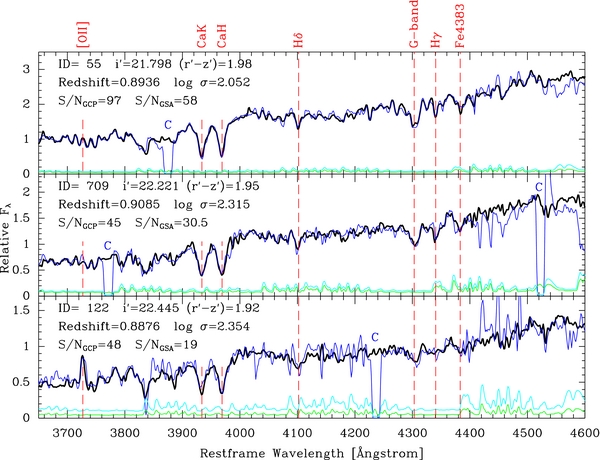
Figure 30. Spectra from the GCP data and the GSA data of the same three galaxies. The GSA spectra have been scaled to the level of the GCP spectra. Black: GCP spectra; dark blue: GSA spectra; green: four times the noise of the GCP spectra; light blue: four times the noise of the GSA spectra. The chip gaps in the GSA data are marked with "C."
Download figure:
Standard image High-resolution imageFinally, we compare the GCP and the GSA data to ensure consistency and in order to provide better estimates of the uncertainties on the line indices from GSA data than those resulting from estimates based on the local S/N of the spectra. There are 23 galaxies in common between the GCP data and the GSA data for RXJ1226.9+3332. Our approach is to calibrate the GSA data to consistency with the GCP data, since the latter has higher S/N and better resolution. Figure 31 shows the comparison of the redshifts, velocity dispersions and CN3883 for these two data sets. Table 20 summarizes the comparisons. The velocity dispersions derived from the GSA data are systematically 0.022 smaller in log σ than found from the GCP data. Even though this is below the 0.026 possible systematic errors in the low-redshift comparison samples (cf. Jørgensen et al. 2005), we have chosen to correct the GSA data for the offset. The scatter for the comparison of the velocity dispersions is within the expected scatter based on the uncertainties as derived from the kinematics fits. None of the offsets for the line indices are significant. As for the GCP data, we use the scatter to estimate the uncertainties. We use the adopted uncertainties for the GCP data (Table 19). The resulting uncertainties listed in Table 20 are a factor of two to three larger than the uncertainties on the GCP data. The higher order Balmer lines are not included in the table as none of the GSA spectra result in measurements if these indices used in the analysis.

Figure 31. Comparison of the GCP data and the GSA data for the spectral parameters used in the analysis and with the most galaxies in common. In panels (b) and (c)—filled boxes: S/NGSA ⩾ 20 per Å in the rest frame; open boxes: S/NGSA < 20.
Download figure:
Standard image High-resolution imageTable 20. Spectroscopic Comparisons
| Parameter | N | GCP−GSAa | rms | σadoptb |
|---|---|---|---|---|
| Redshift | 23 | 0.0003 | 0.0003 | |
| log σ | 23 | 0.035 | 0.054 | |
| log σc | 18 | 0.022 | 0.046 | |
| CN3883 | 20 | 0.002 | 0.045 | 0.042 |
| log CaHK | 19 | −0.005 | 0.071 | 0.056 |
| D4000 | 21 | −0.032 | 0.084 | 0.077 |
| log G4300 | 14 | −0.034 | 0.10 | 0.096 |
| log Fe4383 | 4 | −0.10 | 0.20 | 0.18 |
Notes. aMedian difference of data from the GCP data and the GSA data. bAdopted uncertainties on line indices from the GSA data. cS/NGSA ⩾ 20.
Download table as: ASCIITypeset image
For galaxies with detectable emission from [O ii] we determined the equivalent width of the [O ii]λλ3726,3729 doublet. With an instrumental resolution of σ ≈ 3 Å (FWHM ≈7 Å), the doublet is not resolved in our spectra and we refer to it simply as the "[O ii] line."
B.8. Systematic Effects in Derived Velocity Dispersions
In Jørgensen et al. (2005) we used simulated spectra to determine how the input S/N and the galaxy velocity dispersion relative to the instrumental resolution affected the determined velocity dispersions. Those simulations are also applicable to the RXJ1226.9+3332 data obtained for the GCP, as these have similar instrumental resolution and S/N as the RXJ0152.7−1357 data in Jørgensen et al. The instrumental resolution of the GCP data for RXJ1226.9+3332 and RXJ0152.7−1357 is about 120 km s−1. However, both the RXJ1226.9+3332 GSA data and the MS0451.6−0305 GCP data have worse instrumental resolutions, both equivalent to about 145 km s−1 at 4300 Å in the rest frame of the galaxies in the clusters. Further, the GSA data in general have lower S/N than the GCP data and are subject to larger effects from systematic sky subtraction errors. To estimate the effect of the worse instrumental resolution we ran simulations in a similar fashion as described in Jørgensen et al., using the observed noise spectrum and the instrumental resolution relevant for the data set. We then simulated spectra with S/N between 10 and 50 Å−1 in the rest frame, and input velocity dispersions between 50 and 300 km s−1. For these simulations we used a mix of the G1V and K0III template stars each contributing half the flux to the simulated spectrum. Each combination of S/N and input velocity dispersion was realized 100 times. We use the median of the output velocity dispersion in the following assessment.
Figure 32 shows the result of the two sets of simulations. The main difference between the simulations for the two high-redshift clusters and for MS0451.6−0305 is difference in the length of the wavelength interval used for the kinematic fitting. The simulations matching the RXJ1226.9+3332 GSA data set (Figures 32(a)–(c)) show a similar dependence on the input velocity dispersions as found for our previous simulations for RXJ0152.7−1257. The thin solid line in Figure 32(a) shows the simulations for RXJ0152.7−1257 from Jørgensen et al. Since the dependence on the input velocity dispersion is approximately is the same for the two sets of simulations, any difference between velocity dispersions derived from the GCP data and the GSA data is expected to be small, as was found in the previous section.

Figure 32. Results from simulations. The systematic error on log σ, Δlog σ = log σoutput − log σinput as a function of the input values log σinput (a) and (d) and as a function of the S/N Å−1 (b) and (f). Panels (c) and (e) show input vs. output values. The simulations in panels (a)–(c) apply to the RXJ1226.9+3332 GSA data, while panels (d)–(e) apply to the MS0451.6−0305 data. The dashed lines in panels (a) and (d) mark the median values of Δlog σ. The solid line in panel (a) shows the simulations for the RXJ0152.7−1357 data from Jørgensen et al. (2005). The solid line in panel (e) shows the adopted correction for the systematic errors for the MS0451.6−0305 data; see Equation (B4).
Download figure:
Standard image High-resolution imageThe simulations matching the MS0451.6−0305 data set (Figures 32(d)–(f)) show that velocity dispersions are systematically derived too small, and that the systematic error increases with decreasing input velocity dispersion. For input velocity dispersion log σ > 1.9 we establish a correction function:
The function is shown as the solid line in Figure 32(f). Since the size of this correction is similar to or larger than typical inconsistencies between different data sets, we have chosen to apply the correction to the measured velocity dispersions for MS0451.6−0305 galaxies. The correction is applied to the value in column log σcor (together with the aperture correction) in Table 21, while the column log σ lists the raw measure values.
Table 21. MS0451.6−0305: Results from Template Fitting
| ID | Redshift | Member a | log σ | log σcorb | σlog σ | Template Fractions | χ2 | S/Nc | ||
|---|---|---|---|---|---|---|---|---|---|---|
| B8V | G1V | K0III | ||||||||
| 12 | 0.5508 | 1 | 2.178 | 2.233 | 0.044 | 0.33 | 0.26 | 0.40 | 2.6 | 44.7 |
| 153 | 0.5475 | 1 | 2.236 | 2.285 | 0.029 | 0.00 | 0.59 | 0.41 | 6.7 | 77.2 |
| 220 | 0.8259 | 0 | ... | ... | ... | ... | ... | ... | ... | 45.4 |
| 234 | 0.3554 | 0 | ... | ... | ... | ... | ... | ... | ... | 75.4 |
| 258 | 0.5408 | 1 | 2.081 | 2.154 | 0.056 | 0.35 | 0.58 | 0.07 | 2.1 | 41.4 |
| 299 | 0.5407 | 1 | 2.429 | 2.486 | 0.022 | 0.12 | 0.31 | 0.58 | 12.6 | 197.5 |
| 309 | 0.5417 | 1 | 2.026 | 2.114 | 0.035 | 0.00 | 0.74 | 0.26 | 1.5 | 34.2 |
| 323 | 0.5891 | 0 | ... | ... | ... | ... | ... | ... | ... | 114.3 |
| 386 | 0.8849 | 0 | ... | ... | ... | ... | ... | ... | ... | 14.7 |
| 468 | 1.1792 | 0 | ... | ... | ... | ... | ... | ... | ... | 25.5 |
| 554 | 0.5364 | 1 | 2.035 | 2.120 | 0.035 | 0.03 | 0.70 | 0.27 | 2.5 | 50.5 |
| 600 | 0.5371 | 1 | 1.998 | 2.094 | 0.076 | 0.00 | 0.68 | 0.32 | 4.3 | 92.2 |
| 606 | 0.5684 | 0 | ... | ... | ... | ... | ... | ... | ... | 71.1 |
| 684 | 0.5423 | 1 | 1.936 | 2.054 | 0.064 | 0.18 | 0.30 | 0.52 | 3.4 | 52.8 |
| 716 | 0.5474 | 1 | 1.972 | 2.077 | 0.060 | 0.00 | 0.57 | 0.43 | 2.3 | 46.4 |
| 722 | 0.5473 | 1 | 2.092 | 2.162 | 0.088 | 0.47 | 0.53 | 0.00 | 2.3 | 29.2 |
| 833 | 0.9496 | 0 | ... | ... | ... | ... | ... | ... | ... | 16.1 |
| 836 | 0.3676 | 0 | ... | ... | ... | ... | ... | ... | ... | 44.0 |
| 897 | 0.5457 | 1 | 2.106 | 2.174 | 0.040 | 0.00 | 0.49 | 0.51 | 4.0 | 65.5 |
| 901 | 1.0656 | 0 | ... | ... | ... | ... | ... | ... | ... | 95.0 |
| 921 | 0.5494 | 1 | 2.223 | 2.274 | 0.036 | 0.00 | 0.73 | 0.27 | 11.9 | 139.0 |
| 971 | 0.5437 | 1 | 2.140 | 2.201 | 0.039 | 0.00 | 0.66 | 0.34 | 10.4 | 103.4 |
| 1002 | 0.5477 | 1 | 1.974 | 2.078 | 0.034 | 0.00 | 0.81 | 0.19 | 2.1 | 44.9 |
| 1082 | 0.5501 | 1 | 2.307 | 2.355 | 0.029 | 0.00 | 0.44 | 0.56 | 7.7 | 119.1 |
| 1156 | 0.5397 | 1 | 2.020 | 2.109 | 0.073 | 0.09 | 0.48 | 0.43 | 2.1 | 43.4 |
| 1204 | 0.5342 | 1 | 2.002 | 2.096 | 0.045 | 0.00 | 0.62 | 0.38 | 4.4 | 77.4 |
| 1331 | 0.5362 | 1 | 2.059 | 2.137 | 0.041 | 0.39 | 0.51 | 0.09 | 2.4 | 74.6 |
| 1491 | 0.5369 | 1 | 2.337 | 2.385 | 0.035 | 0.00 | 0.49 | 0.51 | 1.9 | 37.3 |
| 1497 | 0.5318 | 1 | 2.294 | 2.342 | 0.042 | 0.00 | 0.52 | 0.48 | 7.9 | 137.3 |
| 1500 | 0.5391 | 1 | 2.276 | 2.324 | 0.035 | 0.10 | 0.22 | 0.67 | 5.1 | 77.5 |
| 1507 | 0.5392 | 1 | 2.350 | 2.399 | 0.037 | 0.14 | 0.04 | 0.82 | 8.7 | 105.0 |
| 1584 | 0.9546 | 0 | ... | ... | ... | ... | ... | ... | ... | 14.5 |
| 1594 | 0.5373 | 1 | 2.221 | 2.272 | 0.048 | 0.00 | 0.61 | 0.39 | 5.3 | 84.7 |
| 1638 | 0.5473 | 1 | 2.208 | 2.260 | 0.037 | 0.00 | 0.36 | 0.64 | 5.2 | 85.7 |
| 1720 | 0.5389 | 1 | 2.389 | 2.441 | 0.022 | 0.00 | 0.31 | 0.69 | 8.9 | 148.4 |
| 1723 | 0.5372 | 1 | 2.177 | 2.232 | 0.024 | 0.21 | 0.59 | 0.19 | 7.6 | 131.0 |
| 1753 | 0.5305 | 1 | 2.221 | 2.272 | 0.043 | 0.00 | 0.40 | 0.60 | 3.7 | 77.1 |
| 1823 | 0.5306 | 1 | 2.157 | 2.215 | 0.048 | 0.00 | 0.43 | 0.57 | 5.7 | 90.3 |
| 1904 | 0.5391 | 1 | 2.273 | 2.321 | 0.021 | 0.00 | 0.45 | 0.55 | 4.6 | 89.0 |
| 1931 | 0.5550 | 1 | 2.054 | 2.133 | 0.033 | 0.00 | 0.52 | 0.48 | 3.8 | 73.9 |
| 1952 | 0.5494 | 1 | 2.292 | 2.340 | 0.030 | 0.18 | 0.20 | 0.61 | 8.1 | 117.6 |
| 2031 | 0.5315 | 1 | 2.375 | 2.426 | 0.032 | 0.00 | 0.42 | 0.58 | 4.4 | 84.3 |
| 2032 | 0.5114 | 0 | ... | ... | ... | ... | ... | ... | ... | 74.3 |
| 2127 | 0.5241 | 1 | 2.031 | 2.116 | 0.041 | 0.58 | 0.35 | 0.07 | 4.9 | 102.6 |
| 2166 | 0.5319 | 1 | 2.044 | 2.126 | 0.058 | 0.48 | 0.28 | 0.24 | 3.3 | 62.3 |
| 2223 | 0.5450 | 1 | 1.937 | 2.055 | 0.037 | 0.00 | 0.57 | 0.43 | 2.2 | 44.2 |
| 2230 | 0.9199 | 0 | ... | ... | ... | ... | ... | ... | ... | 25.4 |
| 2240 | 0.5469 | 1 | 1.974 | 2.078 | 0.082 | 0.17 | 0.48 | 0.36 | 2.2 | 30.6 |
| 2491 | 0.9192 | 0 | ... | ... | ... | ... | ... | ... | ... | 39.2 |
| 2561 | 1.0493 | 0 | ... | ... | ... | ... | ... | ... | ... | 16.5 |
| 2563 | 0.5315 | 1 | 2.300 | 2.348 | 0.049 | 0.00 | 0.45 | 0.55 | 5.1 | 74.1 |
| 2645 | 0.5300 | 1 | 1.964 | 2.071 | 0.048 | 0.37 | 0.42 | 0.21 | 5.8 | 108.3 |
| 2657 | 0.5787 | 0 | ... | ... | ... | ... | ... | ... | ... | 47.3 |
| 2689 | 0.5308 | 1 | 2.101 | 2.169 | 0.037 | 0.00 | 0.59 | 0.41 | 4.8 | 81.1 |
| 2788 | 0.5405 | 1 | 2.020 | 2.109 | 0.039 | 0.00 | 0.42 | 0.58 | 3.4 | 59.7 |
| 2913 | 0.5420 | 1 | 2.344 | 2.392 | 0.020 | 0.00 | 0.57 | 0.43 | 10.1 | 134.0 |
| 2945 | 0.5255 | 1 | 1.911 | 2.039 | 0.061 | 0.00 | 0.60 | 0.40 | 3.8 | 60.9 |
| 3005 | 0.9193 | 0 | ... | ... | ... | ... | ... | ... | ... | 35.5 |
| 3124 | 0.5469 | 1 | 1.987 | 2.087 | 0.045 | 0.13 | 0.49 | 0.37 | 2.2 | 57.8 |
| 3260 | 0.5336 | 1 | 2.245 | 2.294 | 0.039 | 0.16 | 0.20 | 0.64 | 2.5 | 42.5 |
| 3521 | 0.4912 | 0 | ... | ... | ... | ... | ... | ... | ... | 64.2 |
| 3610 | 0.5663 | 0 | ... | ... | ... | ... | ... | ... | ... | 32.5 |
| 3625 | 0.9489 | 0 | ... | ... | ... | ... | ... | ... | ... | 28.9 |
| 3635 | 0.7668 | 0 | ... | ... | ... | ... | ... | ... | ... | 13.7 |
| 3697 | 0.5674 | 0 | ... | ... | ... | ... | ... | ... | ... | 23.3 |
| 3724 | 0.5417 | 1 | 1.977 | 2.080 | 0.036 | 0.00 | 0.58 | 0.42 | 2.5 | 59.2 |
| 3749 | 0.5422 | 1 | 2.028 | 2.115 | 0.047 | 0.19 | 0.38 | 0.44 | 2.5 | 47.1 |
| 3792 | 0.8996 | 0 | ... | ... | ... | ... | ... | ... | ... | 19.4 |
| 3857 | 0.5348 | 1 | 2.103 | 2.171 | 0.057 | 0.00 | 0.47 | 0.53 | 3.5 | 60.7 |
| 3906 | 1.2846 | 0 | ... | ... | ... | ... | ... | ... | ... | 21.4 |
Notes.
aAdopted membership—1: galaxy is a member of MS0451.6−0305; 0: galaxy is not a member of MS0451.6−0305.
bVelocity dispersions corrected for systematic effects, see Appendix B.8, and corrected to a standard size aperture equivalent to a circular aperture with a diameter of 34 at the distance of the Coma cluster.
cS/N per Å in the rest frame of the galaxy. The wavelength interval was chosen based on the redshift of the galaxy as follows—redshift less than 0.4: 4500–5500 Å; redshift 0.4–0.6: 4100–5500 Å; redshift 0.75–1.1: 3800–4300 Å; redshift larger than 1.1: 3800–4000 Å.
B.9. Final Calibrated Spectroscopic Parameters
Tables 21–24 list the results from the template fitting and the derived line indices. For RXJ1226.9+3332 galaxies included in both the GCP and the GSA data, only the values from the GCP data are listed. The GSA velocity dispersions are calibrated to consistency with the GCP data as explained in Appendix B.7.
Table 22. MS0451.6−0305: Line Indices and EW[O ii] for Cluster Members
| ID | CN3883 | CaHK | D4000 | HδA | CN1 | CN2 | G4300 | HγA | Fe4383 | C4668 | Hβ | HβG | Mgb | Fe5270 | Fe5335 | EW [O ii] |
|---|---|---|---|---|---|---|---|---|---|---|---|---|---|---|---|---|
| 12 | 0.129 | 18.45 | 1.955 | 1.41 | 0.037 | 0.045 | 3.36 | −2.03 | 4.11 | 5.50 | 1.55 | 1.70 | 3.50 | 1.38 | ... | 5.6 |
| 12 | 0.017 | 0.75 | 0.010 | 0.31 | 0.008 | 0.009 | 0.22 | 0.22 | 0.28 | 0.35 | 0.14 | 0.09 | 0.16 | 0.14 | ... | 0.7 |
| 153 | 0.242 | 21.56 | 2.134 | −2.90 | ... | ... | 5.93 | −5.86 | 4.14 | 5.46 | 1.54 | 1.87 | 4.25 | 3.45 | 4.01 | ... |
| 153 | 0.010 | 0.41 | 0.007 | 0.18 | ... | ... | 0.12 | 0.14 | 0.17 | 0.19 | 0.08 | 0.05 | 0.10 | 0.09 | 0.11 | ... |
| 258 | 0.039 | 14.60 | 1.487 | 2.33 | ... | ... | 1.09 | −0.38 | 3.08 | 1.81 | −0.63 | −0.36 | 2.26 | 1.68 | 0.25 | 7.4 |
| 258 | 0.011 | 0.55 | 0.005 | 0.25 | ... | ... | 0.22 | 0.19 | 0.27 | 0.37 | 0.16 | 0.11 | 0.21 | 0.19 | 0.21 | 0.6 |
| 299 | 0.289 | 22.49 | 2.116 | −0.56 | 0.123 | 0.152 | 5.43 | −5.24 | 4.09 | 8.10 | 1.97 | 2.17 | 4.76 | 3.02 | 2.08 | ... |
| 299 | 0.004 | 0.16 | 0.002 | 0.07 | 0.002 | 0.002 | 0.05 | 0.05 | 0.06 | 0.08 | 0.03 | 0.02 | 0.04 | 0.04 | 0.04 | ... |
| 309 | 0.129 | 20.22 | 1.868 | ... | ... | ... | 3.54 | −2.79 | 3.92 | 3.93 | 2.01 | 2.15 | 2.24 | 2.76 | ... | ... |
| 309 | 0.018 | 0.82 | 0.010 | ... | ... | ... | 0.27 | 0.27 | 0.36 | 0.43 | 0.18 | 0.12 | 0.26 | 0.21 | ... | ... |
| 554 | ... | ... | ... | 0.68 | 0.040 | 0.055 | 4.25 | −3.35 | 3.51 | 4.37 | 2.10 | 2.28 | 2.99 | 2.32 | 1.30 | ... |
| 554 | ... | ... | ... | 0.26 | 0.007 | 0.008 | 0.19 | 0.19 | 0.25 | 0.28 | 0.11 | 0.08 | 0.18 | 0.15 | 0.16 | ... |
| 600 | 0.090 | 10.41 | 1.500 | −1.22 | 0.033 | 0.030 | 1.63 | −2.05 | 2.44 | −0.27 | 1.05 | 1.55 | 1.86 | 1.78 | 1.04 | ... |
| 600 | 0.006 | 0.31 | 0.003 | 0.15 | 0.004 | 0.004 | 0.10 | 0.10 | 0.14 | 0.16 | 0.07 | 0.05 | 0.10 | 0.09 | 0.09 | ... |
| 684 | 0.159 | 21.70 | 1.874 | 0.84 | 0.029 | 0.062 | 3.77 | −2.51 | 4.40 | 4.19 | 2.80 | 2.99 | 3.26 | 3.31 | 3.07 | ... |
| 684 | 0.012 | 0.52 | 0.007 | 0.23 | 0.006 | 0.007 | 0.17 | 0.17 | 0.21 | 0.29 | 0.12 | 0.07 | 0.17 | 0.14 | 0.14 | ... |
| 716 | 0.220 | 20.60 | 1.865 | −0.24 | 0.043 | 0.069 | 4.30 | −3.66 | 4.36 | 4.09 | 1.83 | 2.15 | 2.66 | 2.97 | ... | ... |
| 716 | 0.014 | 0.61 | 0.008 | 0.27 | 0.007 | 0.007 | 0.19 | 0.21 | 0.27 | 0.33 | 0.14 | 0.09 | 0.19 | 0.16 | ... | ... |
| 722 | 0.096 | 9.76 | 1.398 | 4.82 | ... | ... | 0.67 | 1.25 | 0.14 | 2.01 | −3.18 | −2.88 | 0.20 | 0.29 | ... | 16.8 |
| 722 | 0.014 | 0.76 | 0.006 | 0.30 | ... | ... | 0.27 | 0.24 | 0.36 | 0.54 | 0.28 | 0.19 | 0.34 | 0.28 | ... | 0.8 |
| 897 | ... | ... | ... | ... | ... | ... | 5.30 | −5.04 | 3.88 | 5.13 | 1.86 | 2.07 | 3.59 | 3.33 | 3.83 | ... |
| 897 | ... | ... | ... | ... | ... | ... | 0.14 | 0.15 | 0.19 | 0.23 | 0.10 | 0.06 | 0.13 | 0.11 | 0.13 | ... |
| 921 | 0.274 | 22.87 | 2.064 | −0.64 | 0.105 | 0.126 | 4.83 | −5.01 | 4.90 | 6.08 | 2.06 | 2.28 | 4.25 | 3.02 | 2.67 | ... |
| 921 | 0.005 | 0.21 | 0.003 | 0.10 | 0.002 | 0.003 | 0.07 | 0.07 | 0.09 | 0.11 | 0.04 | 0.03 | 0.06 | 0.05 | 0.07 | ... |
| 971 | ... | ... | ... | −1.20 | 0.115 | 0.143 | 5.41 | −5.40 | 3.79 | 5.67 | 1.09 | 1.43 | 4.20 | 2.93 | 2.31 | ... |
| 971 | ... | ... | ... | 0.13 | 0.003 | 0.004 | 0.09 | 0.10 | 0.12 | 0.14 | 0.06 | 0.04 | 0.08 | 0.07 | 0.08 | ... |
| 1002 | ... | 20.18 | ... | 0.96 | ... | 0.051 | 4.66 | −3.05 | 3.42 | 5.43 | 2.32 | 2.57 | 3.59 | 2.55 | ... | ... |
| 1002 | ... | 0.62 | ... | 0.27 | ... | 0.008 | 0.19 | 0.21 | 0.28 | 0.33 | 0.14 | 0.09 | 0.19 | 0.16 | ... | ... |
| 1082 | 0.244 | 21.64 | 2.041 | −0.94 | 0.085 | 0.108 | 5.97 | −6.05 | 3.86 | 6.55 | 1.85 | 2.00 | 3.65 | 3.18 | 3.12 | ... |
| 1082 | 0.006 | 0.25 | 0.004 | 0.11 | 0.003 | 0.003 | 0.07 | 0.09 | 0.11 | 0.13 | 0.05 | 0.03 | 0.07 | 0.06 | 0.08 | ... |
| 1156 | ... | 8.59 | 1.367 | −1.31 | 0.091 | 0.118 | 2.74 | −5.68 | 4.79 | 6.39 | 1.29 | 1.36 | 2.52 | 2.23 | 1.28 | ... |
| 1156 | ... | 0.57 | 0.004 | 0.28 | 0.007 | 0.008 | 0.21 | 0.22 | 0.28 | 0.33 | 0.14 | 0.10 | 0.21 | 0.17 | 0.19 | ... |
| 1204 | 0.194 | 22.33 | 2.065 | 0.35 | 0.066 | 0.080 | 5.72 | −5.13 | 5.06 | 6.79 | 1.77 | 2.23 | 4.29 | 1.92 | 2.00 | ... |
| 1204 | 0.010 | 0.41 | 0.006 | 0.18 | 0.005 | 0.005 | 0.12 | 0.13 | 0.17 | 0.19 | 0.08 | 0.05 | 0.12 | 0.10 | 0.11 | ... |
| 1331 | ... | 18.12 | ... | 5.10 | ... | ... | 2.08 | 2.06 | 2.21 | −0.27 | 3.79 | 3.96 | 2.78 | 1.86 | 1.99 | ... |
| 1331 | ... | 0.30 | ... | 0.13 | ... | ... | 0.12 | 0.11 | 0.16 | 0.19 | 0.08 | 0.05 | 0.13 | 0.12 | 0.12 | ... |
| 1491 | 0.176 | 21.04 | 2.019 | −2.63 | 0.141 | 0.166 | 6.23 | −4.91 | 5.57 | 5.57 | 1.08 | 1.50 | 4.77 | 1.69 | 3.00 | ... |
| 1491 | 0.021 | 0.85 | 0.013 | 0.37 | 0.009 | 0.010 | 0.25 | 0.28 | 0.34 | 0.37 | 0.16 | 0.11 | 0.25 | 0.20 | 0.20 | ... |
| 1497 | 0.233 | 23.08 | 1.941 | 0.43 | 0.041 | 0.067 | 4.73 | −3.47 | 3.15 | 4.79 | 2.33 | 2.47 | 3.74 | 2.39 | 1.61 | ... |
| 1497 | 0.005 | 0.21 | 0.003 | 0.10 | 0.003 | 0.003 | 0.07 | 0.07 | 0.09 | 0.10 | 0.05 | 0.03 | 0.06 | 0.06 | 0.06 | ... |
| 1500 | 0.247 | 23.35 | 2.136 | −1.16 | 0.126 | 0.160 | 5.60 | −6.00 | 5.41 | 7.34 | 1.44 | 1.84 | 5.04 | 2.98 | 3.13 | ... |
| 1500 | 0.010 | 0.40 | 0.007 | 0.19 | 0.005 | 0.005 | 0.12 | 0.13 | 0.15 | 0.18 | 0.08 | 0.05 | 0.11 | 0.09 | 0.10 | ... |
| 1507 | 0.256 | 22.50 | 2.024 | −0.93 | 0.126 | 0.166 | 4.95 | −5.57 | 5.14 | 6.87 | 1.71 | 1.93 | 3.88 | 2.61 | 2.78 | ... |
| 1507 | 0.007 | 0.29 | 0.004 | 0.14 | 0.004 | 0.004 | 0.09 | 0.10 | 0.11 | 0.13 | 0.06 | 0.04 | 0.08 | 0.07 | 0.07 | ... |
| 1594 | 0.251 | 22.21 | 2.076 | −1.60 | 0.109 | 0.142 | 5.57 | −5.77 | 4.50 | 6.68 | 1.96 | 2.23 | 4.79 | 2.14 | 1.27 | ... |
| 1594 | 0.009 | 0.36 | 0.006 | 0.17 | 0.004 | 0.005 | 0.11 | 0.12 | 0.15 | 0.16 | 0.07 | 0.05 | 0.11 | 0.09 | 0.10 | ... |
| 1638 | 0.215 | 20.45 | 1.986 | −0.92 | 0.138 | 0.161 | 5.21 | −4.93 | 4.51 | 6.15 | 2.30 | 2.37 | 3.65 | 3.00 | 2.45 | ... |
| 1638 | 0.008 | 0.35 | 0.005 | 0.15 | 0.004 | 0.004 | 0.11 | 0.12 | 0.15 | 0.17 | 0.07 | 0.04 | 0.10 | 0.08 | 0.11 | ... |
| 1720 | 0.243 | 19.15 | 1.926 | −1.14 | 0.111 | 0.133 | 5.06 | −5.52 | 4.47 | 6.22 | 1.52 | 1.83 | 4.31 | 2.27 | 2.59 | ... |
| 1720 | 0.005 | 0.20 | 0.003 | 0.10 | 0.002 | 0.003 | 0.06 | 0.07 | 0.09 | 0.10 | 0.04 | 0.03 | 0.06 | 0.05 | 0.06 | ... |
| 1723 | ... | ... | ... | 2.79 | ... | ... | 3.38 | −0.93 | 3.42 | 3.97 | 2.66 | 2.90 | 3.79 | 2.13 | 1.83 | ... |
| 1723 | ... | ... | ... | 0.09 | ... | ... | 0.07 | 0.07 | 0.10 | 0.11 | 0.05 | 0.03 | 0.07 | 0.06 | 0.07 | ... |
| 1753 | 0.124 | 11.80 | 1.404 | −0.26 | 0.049 | 0.040 | 1.95 | −3.17 | 2.38 | 4.14 | 1.49 | 1.70 | 3.24 | 1.89 | 1.42 | ... |
| 1753 | 0.007 | 0.38 | 0.003 | 0.18 | 0.004 | 0.005 | 0.12 | 0.13 | 0.17 | 0.19 | 0.09 | 0.06 | 0.11 | 0.11 | 0.12 | ... |
| 1823 | 0.260 | 22.18 | 2.151 | −1.33 | 0.103 | 0.127 | 5.09 | −4.55 | 3.66 | 7.50 | 1.90 | 1.98 | 4.56 | 2.44 | 2.27 | ... |
| 1823 | 0.009 | 0.35 | 0.006 | 0.16 | 0.004 | 0.005 | 0.12 | 0.12 | 0.14 | 0.15 | 0.07 | 0.05 | 0.09 | 0.09 | 0.09 | ... |
| 1904 | 0.280 | 22.52 | 2.054 | −2.77 | ... | ... | 6.00 | −5.73 | 4.53 | 6.07 | 1.28 | 1.58 | 4.70 | 2.64 | 2.31 | ... |
| 1904 | 0.008 | 0.35 | 0.005 | 0.18 | ... | ... | 0.11 | 0.12 | 0.14 | 0.16 | 0.07 | 0.04 | 0.10 | 0.08 | 0.09 | ... |
| 1931 | 0.233 | 21.22 | 1.969 | −0.72 | ... | ... | 5.15 | −5.06 | 3.55 | 5.20 | 1.58 | 1.89 | 4.00 | 2.36 | 1.36 | ... |
| 1931 | 0.009 | 0.38 | 0.005 | 0.17 | ... | ... | 0.12 | 0.14 | 0.18 | 0.21 | 0.08 | 0.05 | 0.10 | 0.10 | 0.14 | ... |
| 1952 | 0.238 | 20.77 | 2.001 | −0.04 | 0.090 | 0.119 | 4.55 | −4.27 | 4.41 | 7.29 | 2.11 | 2.31 | 3.95 | 3.48 | 3.64 | ... |
| 1952 | 0.006 | 0.25 | 0.004 | 0.11 | 0.003 | 0.003 | 0.08 | 0.08 | 0.11 | 0.13 | 0.05 | 0.03 | 0.07 | 0.06 | 0.08 | ... |
| 2031 | 0.297 | 22.35 | 2.130 | 0.03 | 0.085 | 0.119 | 5.22 | −4.90 | 5.22 | 7.01 | 1.55 | 1.98 | 4.55 | 2.71 | 2.08 | ... |
| 2031 | 0.010 | 0.38 | 0.006 | 0.16 | 0.004 | 0.005 | 0.12 | 0.13 | 0.15 | 0.17 | 0.08 | 0.05 | 0.10 | 0.09 | 0.10 | ... |
| 2127 | 0.048 | 10.43 | 1.196 | 4.63 | ... | ... | 0.65 | 1.85 | 0.73 | 2.41 | −1.35 | −1.25 | 2.77 | 1.63 | 1.56 | ... |
| 2127 | 0.003 | 0.18 | 0.001 | 0.08 | ... | ... | 0.08 | 0.07 | 0.11 | 0.13 | 0.07 | 0.05 | 0.11 | 0.10 | 0.10 | ... |
| 2166 | 0.066 | 10.36 | 1.389 | 1.39 | ... | ... | 1.19 | −0.04 | 2.12 | 3.14 | −4.14 | −3.99 | 3.30 | 2.95 | 1.84 | 11.8 |
| 2166 | 0.007 | 0.38 | 0.003 | 0.17 | ... | ... | 0.15 | 0.14 | 0.20 | 0.24 | 0.12 | 0.09 | 0.14 | 0.14 | 0.15 | 1.5 |
| 2223 | 0.175 | 19.80 | 1.890 | 1.14 | ... | 0.039 | 4.42 | −4.80 | 4.97 | 5.09 | 2.00 | 2.41 | 4.40 | 2.76 | ... | ... |
| 2223 | 0.014 | 0.62 | 0.008 | 0.26 | ... | 0.008 | 0.21 | 0.23 | 0.29 | 0.34 | 0.14 | 0.09 | 0.17 | 0.16 | ... | ... |
| 2240 | 0.143 | 21.85 | 1.908 | 0.38 | 0.042 | 0.038 | 3.57 | −2.53 | 3.21 | 4.48 | 2.00 | 1.98 | 4.21 | 2.90 | ... | ... |
| 2240 | 0.022 | 0.94 | 0.013 | 0.41 | 0.010 | 0.011 | 0.27 | 0.30 | 0.41 | 0.50 | 0.21 | 0.13 | 0.25 | 0.23 | ... | ... |
| 2563 | 0.213 | 19.82 | 1.936 | −1.02 | ... | ... | 5.13 | −4.85 | 3.51 | 4.97 | 1.99 | 2.25 | 3.33 | 2.68 | 1.94 | ... |
| 2563 | 0.010 | 0.43 | 0.006 | 0.20 | ... | ... | 0.14 | 0.14 | 0.17 | 0.19 | 0.09 | 0.06 | 0.12 | 0.11 | 0.11 | ... |
| 2645 | 0.094 | 13.26 | 1.488 | 2.02 | ... | ... | 2.36 | −1.43 | 2.59 | 2.75 | −1.98 | −1.76 | 3.17 | 1.85 | 1.82 | 12.0 |
| 2645 | 0.004 | 0.24 | 0.002 | 0.11 | ... | ... | 0.09 | 0.08 | 0.11 | 0.13 | 0.07 | 0.05 | 0.09 | 0.08 | 0.08 | 0.7 |
| 2689 | 0.300 | 26.61 | 2.216 | −2.82 | ... | ... | 6.09 | −6.95 | 6.37 | 5.65 | 1.53 | 1.90 | 4.89 | 2.18 | 2.66 | 13.8 |
| 2689 | 0.012 | 0.42 | 0.008 | 0.21 | ... | ... | 0.13 | 0.15 | 0.16 | 0.17 | 0.08 | 0.05 | 0.10 | 0.10 | 0.10 | 1.2 |
| 2788 | 0.241 | 20.96 | 2.079 | −0.24 | 0.066 | 0.085 | 5.15 | −5.10 | 5.44 | 6.32 | 2.16 | 2.29 | 3.44 | 2.88 | 2.85 | ... |
| 2788 | 0.013 | 0.53 | 0.008 | 0.23 | 0.006 | 0.007 | 0.15 | 0.17 | 0.21 | 0.24 | 0.10 | 0.07 | 0.13 | 0.12 | 0.13 | ... |
| 2913 | 0.271 | 22.46 | 2.123 | −1.69 | 0.139 | 0.176 | 5.62 | −5.42 | 4.71 | 7.02 | 1.94 | 2.23 | 4.05 | 2.85 | 2.69 | ... |
| 2913 | 0.005 | 0.24 | 0.004 | 0.11 | 0.003 | 0.003 | 0.07 | 0.08 | 0.10 | 0.11 | 0.05 | 0.03 | 0.06 | 0.05 | 0.06 | ... |
| 2945 | 0.213 | 22.87 | 2.051 | 0.73 | 0.059 | 0.086 | 4.76 | −4.64 | 3.76 | 7.01 | 2.38 | 2.65 | 3.90 | 2.53 | 2.84 | ... |
| 2945 | 0.014 | 0.51 | 0.008 | 0.22 | 0.006 | 0.007 | 0.18 | 0.18 | 0.22 | 0.23 | 0.10 | 0.07 | 0.16 | 0.14 | 0.13 | ... |
| 3124 | 0.175 | 21.38 | 1.985 | −0.10 | 0.066 | 0.086 | 4.77 | −3.76 | 3.74 | 6.41 | 1.86 | 2.22 | 3.36 | 3.83 | 2.04 | ... |
| 3124 | 0.012 | 0.50 | 0.007 | 0.22 | 0.005 | 0.006 | 0.15 | 0.16 | 0.20 | 0.26 | 0.11 | 0.07 | 0.14 | 0.12 | 0.15 | ... |
| 3260 | 0.235 | 20.75 | 2.038 | −1.91 | ... | ... | 6.34 | −4.47 | 3.35 | 7.56 | 1.26 | 1.83 | 3.97 | 2.04 | 2.61 | ... |
| 3260 | 0.019 | 0.73 | 0.011 | 0.32 | ... | ... | 0.23 | 0.25 | 0.32 | 0.32 | 0.15 | 0.09 | 0.22 | 0.18 | 0.19 | ... |
| 3724 | 0.230 | 23.02 | 2.030 | −1.99 | ... | ... | 4.67 | −3.95 | 4.23 | 5.57 | 1.99 | 2.60 | 3.29 | 3.21 | 2.27 | ... |
| 3724 | 0.013 | 0.45 | 0.007 | 0.24 | ... | ... | 0.16 | 0.17 | 0.21 | 0.24 | 0.10 | 0.06 | 0.15 | 0.12 | 0.13 | ... |
| 3749 | 0.205 | 21.83 | 1.979 | 0.26 | 0.043 | 0.070 | 4.32 | −2.80 | 2.73 | 4.17 | 2.94 | 3.12 | 4.37 | 3.86 | ... | ... |
| 3749 | 0.015 | 0.58 | 0.009 | 0.28 | 0.007 | 0.008 | 0.20 | 0.20 | 0.27 | 0.31 | 0.12 | 0.07 | 0.18 | 0.14 | ... | ... |
| 3857 | 0.246 | 24.01 | 1.944 | −1.82 | ... | ... | 5.93 | −4.29 | 4.30 | 6.34 | 1.86 | 2.32 | 2.68 | 2.88 | 2.32 | ... |
| 3857 | 0.012 | 0.49 | 0.007 | 0.23 | ... | ... | 0.16 | 0.17 | 0.21 | 0.23 | 0.10 | 0.07 | 0.14 | 0.13 | 0.14 | ... |
Notes. The indices have been corrected for galaxy velocity dispersion and aperture corrected. The second line for each galaxy lists the uncertainties determined from the local S/N.
Table 23. RXJ1226.9+3332: Results from Template Fitting
| ID | Redshift | Member a | log σ | log σcorb | σlog σ | Template Fractions | χ2 | S/Nc | Datad | ||
|---|---|---|---|---|---|---|---|---|---|---|---|
| B8V | G1V | K0III | |||||||||
| 18 | 0.7557 | 0 | ... | ... | ... | ... | ... | ... | ... | 34.9 | 2 |
| 38 | 0.8825 | 1 | 2.122 | 2.171 | 0.150 | 0.34 | 0.53 | 0.13 | 3.3 | 17.2 | 2 |
| 53 | 1.2360 | 0 | ... | ... | ... | ... | ... | ... | ... | 42.8 | 2 |
| 55 | 0.8936 | 1 | 2.027 | 2.052 | 0.034 | 0.13 | 0.44 | 0.43 | 6.4 | 96.9 | 1 |
| 56 | 0.8932 | 1 | 2.068 | 2.093 | 0.063 | 0.22 | 0.53 | 0.25 | 6.9 | 72.3 | 1 |
| 91 | 0.9744 | 0 | ... | ... | ... | ... | ... | ... | ... | 15.9 | 1 |
| 104 | 0.8949 | 1 | 2.162 | 2.187 | 0.047 | 0.16 | 0.36 | 0.48 | 5.3 | 54.2 | 1 |
| 122 | 0.8876 | 1 | 2.329 | 2.354 | 0.052 | 0.29 | 0.36 | 0.35 | 7.4 | 48.1 | 1 |
| 132 | 0.6793 | 0 | ... | ... | ... | ... | ... | ... | ... | 81.3 | 1 |
| 138 | 0.7136 | 0 | ... | ... | ... | ... | ... | ... | ... | 55.5 | 2 |
| 153 | 1.9750 | 0 | ... | ... | ... | ... | ... | ... | ... | 23.3 | 2 |
| 154 | 0.6797 | 0 | ... | ... | ... | ... | ... | ... | ... | 18.5 | 2 |
| 178 | 0.0970 | 0 | ... | ... | ... | ... | ... | ... | ... | 64.1 | 1 |
| 185 | 0.6868 | 0 | ... | ... | ... | ... | ... | ... | ... | 34.8 | 2 |
| 203 | 0.8403 | 0 | ... | ... | ... | ... | ... | ... | ... | 20.4 | 2 |
| 220 | 0.6882 | 0 | ... | ... | ... | ... | ... | ... | ... | 46.6 | 2 |
| 229 | 0.8922 | 1 | 1.997 | 2.045 | 0.073 | 0.22 | 0.44 | 0.35 | 3.7 | 32.0 | 2 |
| 245 | 0.9748 | 0 | ... | ... | ... | ... | ... | ... | ... | 35.3 | 2 |
| 247 | 0.3849 | 0 | ... | ... | ... | ... | ... | ... | ... | 172.0 | 1 |
| 249 | 0.5003 | 0 | ... | ... | ... | ... | ... | ... | ... | 44.2 | 1 |
| 293 | 0.8838 | 1 | 2.254 | 2.278 | 0.045 | 0.19 | 0.41 | 0.40 | 2.9 | 38.4 | 1 |
| 295 | 0.8954 | 1 | 1.948 | 1.973 | 0.060 | 0.29 | 0.33 | 0.38 | 4.5 | 47.6 | 1 |
| 297 | 0.8450 | 0 | ... | ... | ... | ... | ... | ... | ... | 7.2 | 2 |
| 309 | 0.8859 | 1 | 2.294 | 2.343 | 0.147 | 0.00 | 0.20 | 0.80 | 3.2 | 14.5 | 2 |
| 310 | 0.8885 | 1 | 2.096 | 2.145 | 0.088 | 0.18 | 0.49 | 0.33 | 3.5 | 31.8 | 2 |
| 316 | 0.7315 | 0 | ... | ... | ... | ... | ... | ... | ... | 5.1 | 2 |
| 329 | 0.5883 | 0 | ... | ... | ... | ... | ... | ... | ... | 48.8 | 1 |
| 333 | 0.7146 | 0 | ... | ... | ... | ... | ... | ... | ... | 17.4 | 1 |
| 347 | 0.3682 | 0 | ... | ... | ... | ... | ... | ... | ... | 103.5 | 1 |
| 349 | 0.6871 | 0 | ... | ... | ... | ... | ... | ... | ... | 47.3 | 2 |
| 359 | 0.7026 | 0 | ... | ... | ... | ... | ... | ... | ... | 23.8 | 2 |
| 374 | 0.3394 | 0 | ... | ... | ... | ... | ... | ... | ... | 14.6 | 2 |
| 386 | 0.9895 | 0 | ... | ... | ... | ... | ... | ... | ... | 15.2 | 2 |
| 408 | 0.9890 | 0 | ... | ... | ... | ... | ... | ... | ... | 57.3 | 1 |
| 423 | 0.8946 | 1 | 2.309 | 2.358 | 0.040 | 0.11 | 0.54 | 0.34 | 2.0 | 26.9 | 2 |
| 441 | 0.8920 | 1 | 2.046 | 2.071 | 0.044 | 0.10 | 0.66 | 0.24 | 3.1 | 35.1 | 1 |
| 446 | 0.8836 | 1 | 1.936 | 1.985 | 0.067 | 0.18 | 0.75 | 0.07 | 3.7 | 34.8 | 2 |
| 452 | 0.8818 | 1 | 2.107 | 2.132 | 0.075 | 0.55 | 0.27 | 0.18 | 2.8 | 35.0 | 1 |
| 462 | 0.8929 | 1 | 2.071 | 2.120 | 0.072 | 0.00 | 0.40 | 0.60 | 3.9 | 22.1 | 2 |
| 470 | 0.8987 | 1 | 1.991 | 2.040 | 0.096 | 0.16 | 0.49 | 0.34 | 3.3 | 19.8 | 2 |
| 491 | 0.8791 | 1 | 2.216 | 2.240 | 0.046 | 0.00 | 0.50 | 0.49 | 6.3 | 71.8 | 1 |
| 499 | 0.7326 | 0 | ... | ... | ... | ... | ... | ... | ... | 14.5 | 2 |
| 500 | 0.4010 | 0 | ... | ... | ... | ... | ... | ... | ... | 15.7 | 2 |
| 512 | 0.8973 | 1 | 2.085 | 2.133 | 0.059 | 0.00 | 0.33 | 0.67 | 3.9 | 20.7 | 2 |
| 523 | 0.9297 | 0 | ... | ... | ... | ... | ... | ... | ... | 29.5 | 1 |
| 527 | 1.1280 | 0 | ... | ... | ... | ... | ... | ... | ... | 10.1 | 2 |
| 528 | 0.8873 | 1 | 2.297 | 2.346 | 0.058 | 0.44 | 0.27 | 0.29 | 2.0 | 21.2 | 2 |
| 529 | 0.8970 | 1 | 2.361 | 2.386 | 0.028 | 0.00 | 0.45 | 0.55 | 11.3 | 95.5 | 1 |
| 534 | 0.8880 | 1 | 2.437 | 2.485 | 0.051 | 0.00 | 0.79 | 0.21 | 1.9 | 21.6 | 2 |
| 547 | 0.8825 | 1 | 2.079 | 2.127 | 0.227 | 1.00 | 0.00 | 0.00 | 3.3 | 12.1 | 2 |
| 557 | 0.8909 | 1 | 2.205 | 2.230 | 0.086 | 0.00 | 0.59 | 0.41 | 4.4 | 27.0 | 1 |
| 563 | 0.8908 | 1 | 2.528 | 2.553 | 0.017 | 0.10 | 0.30 | 0.60 | 17.4 | 116.3 | 1 |
| 572 | 0.4993 | 0 | ... | ... | ... | ... | ... | ... | ... | 31.8 | 1 |
| 592 | 0.8760 | 1 | ... | ... | ... | ... | ... | ... | ... | 16.0 | 2 |
| 593 | 0.8812 | 1 | 2.127 | 2.176 | 0.074 | 0.00 | 0.89 | 0.11 | 1.8 | 17.5 | 2 |
| 602 | 0.8787 | 1 | 2.085 | 2.110 | 0.040 | 0.42 | 0.58 | 0.00 | 5.0 | 49.7 | 1 |
| 608 | 0.8752 | 1 | 2.160 | 2.209 | 0.038 | 0.00 | 0.89 | 0.11 | 5.9 | 51.8 | 2 |
| 630 | 0.8905 | 1 | ... | ... | ... | ... | ... | ... | ... | 9.3 | 2 |
| 641 | 0.8968 | 1 | 2.088 | 2.136 | 0.042 | 0.00 | 0.57 | 0.43 | 3.7 | 24.4 | 2 |
| 647 | 0.8920 | 1 | 1.963 | 2.012 | 0.098 | 0.12 | 0.62 | 0.26 | 2.1 | 12.3 | 2 |
| 648 | 0.8757 | 1 | 1.933 | 1.957 | 0.046 | 0.00 | 0.73 | 0.27 | 6.0 | 67.5 | 1 |
| 649 | 0.9254 | 0 | ... | ... | ... | ... | ... | ... | ... | 18.7 | 2 |
| 650 | 0.8937 | 1 | 1.963 | 2.012 | 0.076 | 0.32 | 0.47 | 0.21 | 2.9 | 27.6 | 2 |
| 656 | 0.9293 | 0 | ... | ... | ... | ... | ... | ... | ... | 29.4 | 2 |
| 675 | 0.8974 | 1 | 2.151 | 2.176 | 0.064 | 0.22 | 0.40 | 0.38 | 3.6 | 48.8 | 1 |
| 685 | 1.0179 | 0 | ... | ... | ... | ... | ... | ... | ... | 6.5 | 2 |
| 689 | 0.8958 | 1 | 2.337 | 2.386 | 0.068 | 0.00 | 0.41 | 0.59 | 1.8 | 13.6 | 2 |
| 703 | 0.8977 | 1 | 2.415 | 2.440 | 0.017 | 0.12 | 0.30 | 0.58 | 8.5 | 85.7 | 1 |
| 709 | 0.9085 | 1 | 2.290 | 2.315 | 0.038 | 0.21 | 0.46 | 0.32 | 3.4 | 45.4 | 1 |
| 711 | 0.8822 | 1 | 1.797 | 1.822 | 0.090 | 0.62 | 0.38 | 0.00 | 3.3 | 16.4 | 1 |
| 739 | 1.0556 | 0 | ... | ... | ... | ... | ... | ... | ... | 14.2 | 2 |
| 754 | 3.2000 | 0 | ... | ... | ... | ... | ... | ... | ... | 71.6 | 2 |
| 757 | 0.8856 | 1 | 2.230 | 2.279 | 0.116 | 0.00 | 0.74 | 0.26 | 1.3 | 11.3 | 2 |
| 760 | 0.8901 | 1 | 2.310 | 2.335 | 0.037 | 0.15 | 0.47 | 0.38 | 10.4 | 80.0 | 1 |
| 781 | 0.7668 | 0 | ... | ... | ... | ... | ... | ... | ... | 40.0 | 2 |
| 798 | 0.9636 | 0 | ... | ... | ... | ... | ... | ... | ... | 32.3 | 1 |
| 801 | 0.8923 | 1 | 1.939 | 1.987 | 0.076 | 0.13 | 0.65 | 0.22 | 7.2 | 37.3 | 2 |
| 805 | 0.6276 | 0 | ... | ... | ... | ... | ... | ... | ... | 22.4 | 2 |
| 824 | 0.4251 | 0 | ... | ... | ... | ... | ... | ... | ... | 21.3 | 2 |
| 841 | 0.3556 | 0 | ... | ... | ... | ... | ... | ... | ... | 18.7 | 2 |
| 861 | 0.4208 | 0 | ... | ... | ... | ... | ... | ... | ... | 15.1 | 2 |
| 863 | 0.7144 | 0 | ... | ... | ... | ... | ... | ... | ... | 53.7 | 1 |
| 872 | 0.4967 | 0 | ... | ... | ... | ... | ... | ... | ... | 11.3 | 1 |
| 883 | 0.8890 | 1 | 2.112 | 2.160 | 0.085 | 0.21 | 0.56 | 0.24 | 3.3 | 18.6 | 2 |
| 899 | 0.8881 | 1 | 2.181 | 2.205 | 0.036 | 0.10 | 0.63 | 0.27 | 3.9 | 34.9 | 1 |
| 907 | 0.7671 | 0 | ... | ... | ... | ... | ... | ... | ... | 6.8 | 2 |
| 928 | 0.3389 | 0 | ... | ... | ... | ... | ... | ... | ... | 67.8 | 1 |
| 933 | 0.9645 | 0 | ... | ... | ... | ... | ... | ... | ... | 21.5 | 1 |
| 934 | 0.4479 | 0 | ... | ... | ... | ... | ... | ... | ... | 23.0 | 2 |
| 960 | 0.7981 | 0 | ... | ... | ... | ... | ... | ... | ... | 22.1 | 2 |
| 968 | 0.9680 | 0 | ... | ... | ... | ... | ... | ... | ... | 49.8 | 1 |
| 982 | 0.0604 | 0 | ... | ... | ... | ... | ... | ... | ... | 17.0 | 2 |
| 995 | 0.9611 | 0 | ... | ... | ... | ... | ... | ... | ... | 85.4 | 1 |
| 996 | 0.9008 | 1 | 2.132 | 2.157 | 0.053 | 0.21 | 0.51 | 0.29 | 10.0 | 120.8 | 1 |
| 999 | 0.8930 | 1 | 2.004 | 2.053 | 0.118 | 0.57 | 0.43 | 0.00 | 3.7 | 13.1 | 2 |
| 1001 | 0.3377 | 0 | ... | ... | ... | ... | ... | ... | ... | 10.2 | 2 |
| 1005 | 0.8869 | 1 | 2.247 | 2.272 | 0.093 | 0.59 | 0.41 | 0.00 | 2.7 | 23.8 | 1 |
| 1022 | 0.9126 | 1 | 1.956 | 1.980 | 0.244 | 1.00 | 0.00 | 0.00 | 3.2 | 12.3 | 1 |
| 1025 | 0.9030 | 1 | 2.058 | 2.107 | 0.083 | 0.10 | 0.44 | 0.46 | 2.7 | 17.6 | 2 |
| 1027 | 1.0588 | 0 | ... | ... | ... | ... | ... | ... | ... | 10.9 | 2 |
| 1029 | 0.2300 | 0 | ... | ... | ... | ... | ... | ... | ... | 9.5 | 2 |
| 1042 | 0.7028 | 0 | ... | ... | ... | ... | ... | ... | ... | 7.8 | 2 |
| 1047 | 0.8980 | 1 | 2.102 | 2.127 | 0.052 | 0.24 | 0.41 | 0.35 | 3.3 | 43.7 | 1 |
| 1057 | 1.1810 | 0 | ... | ... | ... | ... | ... | ... | ... | 6.9 | 2 |
| 1080 | 0.5303 | 0 | ... | ... | ... | ... | ... | ... | ... | 46.8 | 1 |
| 1083 | 0.5341 | 0 | ... | ... | ... | ... | ... | ... | ... | 37.0 | 1 |
| 1091 | 0.8841 | 1 | 2.001 | 2.050 | 0.089 | 0.46 | 0.00 | 0.54 | 4.4 | 22.0 | 2 |
| 1103 | 0.7028 | 0 | ... | ... | ... | ... | ... | ... | ... | 21.9 | 1 |
| 1157 | 0.7669 | 0 | ... | ... | ... | ... | ... | ... | ... | 11.8 | 1 |
| 1164 | 0.8902 | 1 | 1.960 | 2.009 | 0.077 | 0.21 | 0.48 | 0.31 | 6.1 | 28.5 | 2 |
| 1170 | 0.8911 | 1 | 2.104 | 2.129 | 0.040 | 0.00 | 0.71 | 0.29 | 7.0 | 79.1 | 1 |
| 1175 | 0.9304 | 0 | ... | ... | ... | ... | ... | ... | ... | 94.7 | 1 |
| 1182 | 0.7340 | 0 | ... | ... | ... | ... | ... | ... | ... | 5.4 | 2 |
| 1196 | 0.9438 | 0 | ... | ... | ... | ... | ... | ... | ... | 7.6 | 2 |
| 1199 | 0.9029 | 1 | 2.226 | 2.250 | 0.032 | 0.21 | 0.26 | 0.53 | 5.6 | 64.0 | 1 |
| 1251 | 0.8928 | 1 | 1.966 | 2.015 | 0.081 | 0.00 | 0.90 | 0.10 | 3.9 | 19.0 | 2 |
| 1252 | 0.8997 | 1 | 2.207 | 2.255 | 0.080 | 0.12 | 0.57 | 0.31 | 1.2 | 10.6 | 2 |
| 1253 | 1.0600 | 0 | ... | ... | ... | ... | ... | ... | ... | ... | 1 |
| 1254 | 1.1236 | 0 | ... | ... | ... | ... | ... | ... | ... | 31.8 | 1 |
Notes.
aAdopted membership—1: galaxy is a member of RXJ1226.9+3332; 0: galaxy is not a member of RXJ1226.9+3332.
bVelocity dispersions corrected to a standard size aperture equivalent to a circular aperture with a diameter of 34 at the distance of the Coma cluster.
cS/N per Å in the rest frame of the galaxy. The wavelength interval was 4100–4600 Å, except when wavelength coverage did not allow this typically due to the redshift of the galaxy the following intervals were used—ID 178: 6500–7000 Å; IDs 132, 247, 249, 982, 1029, and 1083: 5000–5500 Å; IDs 527, 1027, and 1057: 3500–4000 Å; IDs 53 and 153: 2500–3000 Å; ID 754: 1500–2000 Å.
dSource of data: (1) GCP; (2) GSA.
Table 24. RXJ1226.9+3332: Line Indices and EW[O ii] for Cluster Members
| ID | CN3883 | CaHK | D4000 | HδA | CN1 | CN2 | G4300 | HγA | Fe4383 | C4668 | EW [O ii] |
|---|---|---|---|---|---|---|---|---|---|---|---|
| 38 | ... | 15.34 | 1.707 | ... | 0.071 | 0.082 | ... | ... | ... | ... | 10.2 |
| 38 | ... | 0.92 | 0.010 | ... | 0.014 | 0.017 | ... | ... | ... | ... | 1.0 |
| 55 | 0.237 | 21.42 | 2.000 | 0.36 | 0.099 | 0.122 | 4.89 | −3.04 | 4.41 | 6.33 | ... |
| 55 | 0.003 | 0.16 | 0.002 | 0.09 | 0.003 | 0.003 | 0.06 | 0.08 | 0.14 | 0.20 | ... |
| 56 | 0.173 | 18.70 | 1.811 | 1.24 | 0.033 | 0.055 | 4.04 | −1.87 | 3.71 | 4.15 | 3.2 |
| 56 | 0.004 | 0.22 | 0.003 | 0.12 | 0.003 | 0.004 | 0.09 | 0.10 | 0.18 | 0.28 | 0.3 |
| 104 | 0.245 | 22.07 | 2.008 | 0.26 | 0.145 | 0.153 | 4.80 | −2.76 | 4.48 | 6.84 | 3.5 |
| 104 | 0.006 | 0.29 | 0.004 | 0.17 | 0.005 | 0.005 | 0.11 | 0.14 | 0.24 | 0.33 | 0.5 |
| 122 | 0.143 | 18.99 | 1.829 | 3.73 | ... | 0.026 | 2.60 | −0.38 | 3.42 | 5.35 | 6.9 |
| 122 | 0.006 | 0.31 | 0.004 | 0.15 | ... | 0.006 | 0.13 | 0.14 | 0.24 | 0.35 | 1.2 |
| 229 | 0.261 | ... | 1.988 | 0.41 | ... | 0.043 | 4.98 | ... | ... | ... | ... |
| 229 | 0.009 | ... | 0.005 | 0.24 | ... | 0.008 | 0.18 | ... | ... | ... | ... |
| 293 | 0.244 | 20.42 | 2.102 | 0.50 | 0.085 | 0.109 | 5.46 | −3.94 | 5.52 | 4.81 | ... |
| 293 | 0.008 | 0.41 | 0.006 | 0.21 | 0.006 | 0.008 | 0.16 | 0.20 | 0.28 | 0.46 | ... |
| 295 | 0.139 | 16.72 | 1.784 | 1.48 | 0.030 | 0.050 | 3.65 | −1.78 | 2.91 | 6.40 | 8.7 |
| 295 | 0.006 | 0.34 | 0.004 | 0.18 | 0.005 | 0.006 | 0.14 | 0.17 | 0.30 | 0.36 | 1.2 |
| 309 | 0.221 | 23.67 | 1.947 | ... | ... | ... | 5.56 | ... | ... | ... | ... |
| 309 | 0.018 | 0.90 | 0.011 | ... | ... | ... | 0.40 | ... | ... | ... | ... |
| 310 | 0.278 | ... | 2.045 | −1.17 | 0.118 | 0.139 | 4.70 | ... | ... | ... | ... |
| 310 | 0.009 | ... | 0.006 | 0.26 | 0.008 | 0.009 | 0.19 | ... | ... | ... | ... |
| 423 | 0.166 | ... | 2.119 | ... | ... | ... | 4.68 | ... | ... | ... | ... |
| 423 | 0.011 | ... | 0.008 | ... | ... | ... | 0.23 | ... | ... | ... | ... |
| 441 | 0.192 | 21.53 | 1.948 | 1.48 | ... | 0.029 | 4.52 | −2.40 | 4.73 | 3.67 | ... |
| 441 | 0.009 | 0.44 | 0.006 | 0.23 | ... | 0.008 | 0.17 | 0.22 | 0.37 | 0.54 | ... |
| 446 | 0.079 | ... | 1.865 | 1.41 | ... | ... | 3.23 | ... | ... | ... | ... |
| 446 | 0.008 | ... | 0.005 | 0.23 | ... | ... | 0.20 | ... | ... | ... | ... |
| 452 | 0.136 | 12.50 | 1.760 | 4.72 | ... | ... | 0.48 | 3.23 | 2.60 | 3.17 | 10.4 |
| 452 | 0.008 | 0.45 | 0.005 | 0.20 | ... | ... | 0.20 | 0.19 | 0.32 | 0.51 | 0.8 |
| 462 | 0.182 | ... | 1.896 | ... | ... | ... | 5.27 | ... | ... | ... | ... |
| 462 | 0.012 | ... | 0.008 | ... | ... | ... | 0.26 | ... | ... | ... | ... |
| 470 | ... | 25.34 | 2.067 | ... | ... | ... | 3.85 | ... | ... | ... | ... |
| 470 | ... | 0.85 | 0.012 | ... | ... | ... | 0.32 | ... | ... | ... | ... |
| 491 | 0.248 | 22.59 | 2.037 | −0.26 | 0.090 | 0.120 | 4.26 | −3.36 | 4.08 | 6.35 | ... |
| 491 | 0.004 | 0.22 | 0.003 | 0.11 | 0.003 | 0.004 | 0.10 | 0.10 | 0.15 | 0.23 | ... |
| 512 | ... | 21.01 | 2.075 | ... | ... | ... | 4.34 | ... | ... | ... | ... |
| 512 | ... | 0.83 | 0.010 | ... | ... | ... | 0.29 | ... | ... | ... | ... |
| 528 | 0.106 | 14.62 | 1.791 | ... | ... | ... | ... | ... | ... | ... | 3.1 |
| 528 | 0.012 | 0.72 | 0.008 | ... | ... | ... | ... | ... | ... | ... | 0.4 |
| 529 | 0.260 | 23.46 | 2.065 | −1.24 | 0.102 | 0.125 | 5.44 | −4.15 | 3.68 | 7.92 | ... |
| 529 | 0.003 | 0.17 | 0.002 | 0.10 | 0.003 | 0.003 | 0.07 | 0.09 | 0.15 | 0.18 | ... |
| 534 | ... | 20.59 | 2.087 | ... | ... | ... | 4.95 | ... | ... | ... | ... |
| 534 | ... | 0.68 | 0.008 | ... | ... | ... | 0.27 | ... | ... | ... | ... |
| 547 | ... | 7.00 | 1.560 | ... | ... | ... | ... | ... | ... | ... | 24.0 |
| 547 | ... | 1.28 | 0.011 | ... | ... | ... | ... | ... | ... | ... | 1.6 |
| 563 | 0.315 | 23.38 | 2.212 | −0.66 | 0.133 | 0.161 | 5.23 | −4.53 | 4.59 | 8.86 | ... |
| 563 | 0.003 | 0.14 | 0.002 | 0.08 | 0.002 | 0.002 | 0.06 | 0.07 | 0.11 | 0.14 | ... |
| 592 | ... | ... | ... | ... | ... | ... | ... | ... | ... | ... | 3.6 |
| 592 | ... | ... | ... | ... | ... | ... | ... | ... | ... | ... | 0.3 |
| 593 | ... | 20.54 | 2.237 | ... | 0.094 | 0.154 | 4.53 | ... | ... | ... | ... |
| 593 | ... | 0.91 | 0.012 | ... | 0.014 | 0.017 | 0.36 | ... | ... | ... | ... |
| 602 | 0.102 | 16.24 | 1.703 | 4.43 | ... | ... | 1.42 | 2.16 | 3.86 | 3.64 | 11.5 |
| 602 | 0.005 | 0.32 | 0.003 | 0.14 | ... | ... | 0.15 | 0.14 | 0.22 | 0.39 | 0.6 |
| 608 | 0.210 | 22.07 | 1.973 | ... | ... | ... | 4.96 | −4.12 | 5.81 | ... | 10.7 |
| 608 | 0.006 | 0.32 | 0.004 | ... | ... | ... | 0.14 | 0.15 | 0.20 | ... | 1.2 |
| 641 | 0.182 | 22.00 | 1.889 | ... | ... | ... | 4.55 | ... | ... | ... | ... |
| 641 | 0.012 | 0.63 | 0.008 | ... | ... | ... | 0.23 | ... | ... | ... | ... |
| 647 | 0.225 | 24.43 | 2.210 | ... | ... | ... | 5.80 | ... | ... | ... | ... |
| 647 | 0.026 | 1.35 | 0.020 | ... | ... | ... | 0.49 | ... | ... | ... | ... |
| 648 | 0.237 | 19.13 | 2.047 | 1.10 | 0.050 | 0.073 | 4.45 | −2.77 | 3.26 | 4.25 | 2.7 |
| 648 | 0.005 | 0.25 | 0.003 | 0.12 | 0.004 | 0.004 | 0.10 | 0.11 | 0.16 | 0.27 | 0.3 |
| 650 | ... | 17.99 | 1.755 | ... | ... | ... | 4.62 | ... | ... | ... | ... |
| 650 | ... | 0.56 | 0.006 | ... | ... | ... | 0.21 | ... | ... | ... | ... |
| 675 | 0.176 | 21.29 | 1.949 | 2.53 | ... | 0.035 | 3.92 | −2.14 | 3.20 | 1.95 | 3.7 |
| 675 | 0.006 | 0.32 | 0.004 | 0.18 | ... | 0.006 | 0.13 | 0.17 | 0.29 | 0.43 | 0.4 |
| 689 | 0.299 | ... | 2.173 | ... | ... | ... | 2.88 | ... | ... | ... | ... |
| 689 | 0.026 | ... | 0.019 | ... | ... | ... | 0.51 | ... | ... | ... | ... |
| 703 | 0.312 | 23.82 | 2.170 | −0.61 | 0.108 | 0.138 | 5.68 | −4.47 | 3.40 | 7.05 | ... |
| 703 | 0.004 | 0.18 | 0.003 | 0.11 | 0.003 | 0.003 | 0.07 | 0.10 | 0.16 | 0.22 | ... |
| 709 | 0.230 | 21.09 | 2.007 | 1.36 | ... | 0.035 | 3.73 | −0.26 | 4.72 | ... | ... |
| 709 | 0.007 | 0.36 | 0.005 | 0.22 | ... | 0.006 | 0.14 | 0.19 | 0.30 | ... | ... |
| 711 | 0.067 | 9.35 | 1.461 | 7.06 | ... | ... | −0.51 | 7.76 | ... | ... | ... |
| 711 | 0.012 | 0.84 | 0.007 | 0.34 | ... | ... | 0.42 | 0.35 | ... | ... | ... |
| 757 | 0.306 | 26.79 | 2.007 | ... | 0.070 | ... | 3.93 | ... | ... | ... | ... |
| 757 | 0.027 | 1.31 | 0.019 | ... | 0.023 | ... | 0.61 | ... | ... | ... | ... |
| 760 | 0.229 | 21.85 | 2.014 | 1.19 | 0.056 | 0.078 | 4.80 | −3.49 | 4.62 | 7.94 | ... |
| 760 | 0.004 | 0.19 | 0.003 | 0.10 | 0.003 | 0.004 | 0.08 | 0.10 | 0.15 | 0.21 | ... |
| 801 | 0.180 | 20.33 | 1.964 | ... | ... | ... | 4.58 | ... | ... | ... | ... |
| 801 | 0.008 | 0.41 | 0.005 | ... | ... | ... | 0.17 | ... | ... | ... | ... |
| 883 | ... | ... | 1.875 | ... | ... | ... | 4.50 | ... | ... | ... | ... |
| 883 | ... | ... | 0.008 | ... | ... | ... | 0.33 | ... | ... | ... | ... |
| 899 | ... | 21.27 | ... | 1.89 | 0.092 | 0.124 | 5.02 | −5.26 | 6.45 | 5.03 | ... |
| 899 | ... | 0.45 | ... | 0.23 | 0.007 | 0.009 | 0.18 | 0.22 | 0.33 | 0.50 | ... |
| 996 | 0.221 | 21.83 | 1.994 | 2.12 | ... | 0.048 | 4.41 | −0.72 | 2.18 | 5.12 | ... |
| 996 | 0.002 | 0.12 | 0.002 | 0.07 | ... | 0.002 | 0.05 | 0.07 | 0.12 | 0.17 | ... |
| 999 | 0.120 | 19.27 | 1.646 | ... | ... | ... | 2.11 | ... | ... | ... | ... |
| 999 | 0.019 | 1.02 | 0.010 | ... | ... | ... | 0.45 | ... | ... | ... | ... |
| 1005 | ... | 8.32 | 1.367 | 3.93 | ... | ... | 1.02 | −1.44 | 1.89 | 1.25 | 33.6 |
| 1005 | ... | 0.58 | 0.005 | 0.28 | ... | ... | 0.27 | 0.30 | 0.55 | 0.98 | 6.7 |
| 1022 | ... | ... | 1.408 | ... | ... | ... | ... | ... | ... | ... | 58.6 |
| 1022 | ... | ... | 0.009 | ... | ... | ... | ... | ... | ... | ... | 4.4 |
| 1025 | ... | 19.24 | ... | ... | ... | ... | 4.31 | ... | ... | ... | ... |
| 1025 | ... | 1.01 | ... | ... | ... | ... | 0.34 | ... | ... | ... | ... |
| 1047 | 0.217 | 22.59 | 1.975 | 1.87 | ... | ... | 3.85 | −0.89 | 2.76 | 5.83 | ... |
| 1047 | 0.007 | 0.37 | 0.005 | 0.21 | ... | ... | 0.15 | 0.19 | 0.34 | 0.49 | ... |
| 1091 | 0.214 | ... | 1.690 | ... | 0.032 | 0.033 | 2.85 | ... | ... | ... | 8.2 |
| 1091 | 0.011 | ... | 0.007 | ... | 0.011 | 0.013 | 0.29 | ... | ... | ... | 1.0 |
| 1164 | 0.151 | ... | 2.072 | ... | ... | ... | 4.90 | ... | ... | ... | ... |
| 1164 | 0.010 | ... | 0.007 | ... | ... | ... | 0.21 | ... | ... | ... | ... |
| 1170 | 0.207 | 20.47 | 1.956 | 1.28 | 0.051 | 0.074 | 4.12 | −2.03 | 4.22 | 8.45 | ... |
| 1170 | 0.004 | 0.20 | 0.003 | 0.10 | 0.003 | 0.004 | 0.08 | 0.10 | 0.16 | 0.22 | ... |
| 1199 | 0.258 | 22.55 | 1.915 | 0.11 | 0.088 | 0.101 | 4.55 | −2.43 | 3.83 | 4.77 | ... |
| 1199 | 0.005 | 0.25 | 0.003 | 0.15 | 0.004 | 0.004 | 0.10 | 0.13 | 0.21 | 0.30 | ... |
| 1251 | 0.045 | 12.13 | 1.935 | ... | ... | ... | 3.47 | ... | ... | ... | ... |
| 1251 | 0.009 | 0.91 | 0.008 | ... | ... | ... | 0.32 | ... | ... | ... | ... |
Notes. The indices have been corrected for galaxy velocity dispersion and aperture corrected. The second line for each galaxy lists the uncertainties determined from the local S/N. ID = 557 and ID = 630 have no reliable line index measurements.
APPENDIX C: PRESENTATION OF THE IMAGING AND SPECTRA FOR MS0451.6−0305 AND RXJ1226.9+3332
Stamp-sized images of the galaxies from the HST/ACS imaging are shown in Figures 33 and 34. The stamps cover the equivalent of 75 kpc × 75 kpc at the distance of the clusters. The panels are labeled to show which galaxies are included in the analysis. The selection criteria are detailed in Section 8. The spectra of the cluster members of MS0451.6−0306 and RXJ1226.9+3332 are shown in Figures 35 and 36. Full figures are available in the online journal.
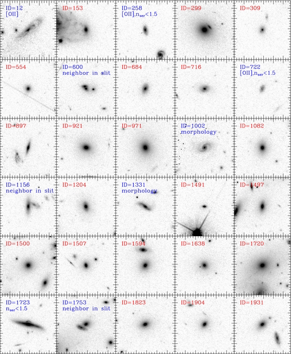
Download figure:
Standard image High-resolution image
Figure 33. HST/ACS images of the MS0451.6−0305 sample in the F814W filter. Each image is 115 × 115. At the distance of MS0451.6−0305 this corresponds to 75 kpc × 75 kpc for our adopted cosmology. North is up and east is to the left. In each panel, the galaxy with the ID listed above the image is located in the center of that image. Red ID: galaxy is included in the analysis; blue ID: galaxy is excluded from the analysis; the reason is listed; see Section 8 for details.
Download figure:
Standard image High-resolution image
Download figure:
Standard image High-resolution image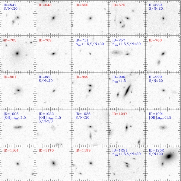
Figure 34. HST/ACS images of the RXJ1226.9+3332 sample in the F814W filter. Each image is 95 × 95. At the distance of RXJ1226.9+3332 this corresponds to 75 kpc × 75 kpc for our adopted cosmology. North is up and east is to the left. In each panel, the galaxy with the ID listed above the image is located in the center of that image. Red ID: galaxy is included in the analysis; blue ID: galaxy is excluded from the analysis; the reason is listed; see Section 8 for details.
Download figure:
Standard image High-resolution image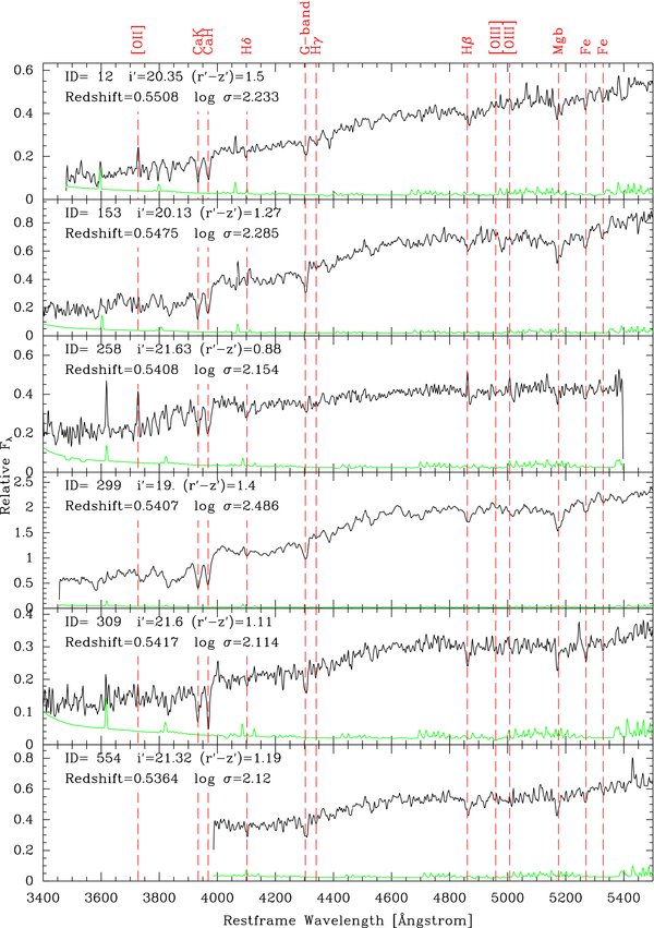
Figure 35.
Spectra of the galaxies that are considered members of MS0451.6−0305. Black lines: the galaxy spectra; green lines: the random noise multiplied with four. At the strong skylines, the random noise underestimates the real noise due to systematic errors in the sky subtraction. Some of the absorption lines are marked. The location of the emission lines [O ii], [O iii]λ4959, and [O iii]λ5007 are also marked, though these lines are only present in some of the galaxies. The spectra shown in this figure have been processed as described in the text, including resampling to just better than critical sampling. (An extended version of this figure is available in the online journal.)
Download figure:
Standard image High-resolution image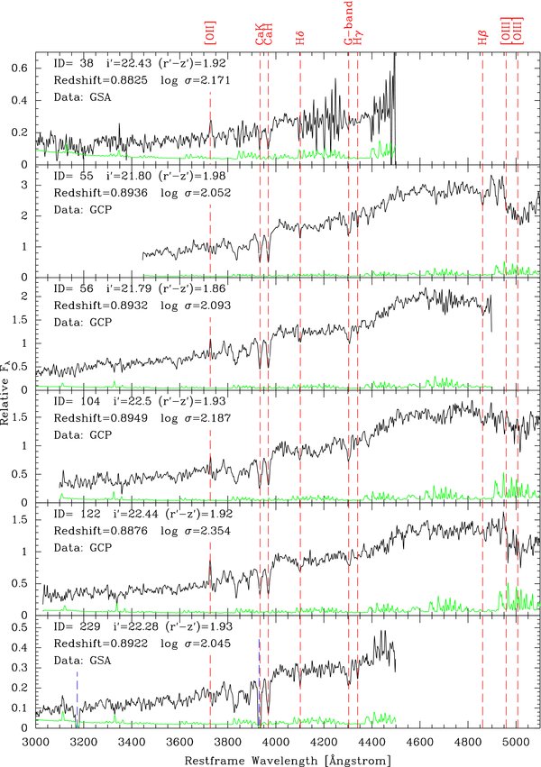
Figure 36.
Spectra of the galaxies that are considered members of RXJ1226.9+3332. The data source (GCP or GSA) is given on the panels. Lines and labeling are the same as in Figure 35. The GSA data are not plotted for rest-frame wavelength larger than 4500 Å as the spectra are affected significantly by systematic sky subtraction errors; see the text for details. For GSA data taken with only one wavelength setting there are gaps in the spectra due to the gaps between the GMOS-N CCDs. These gaps are marked with blue dashed lines. (An extended version of this figure is available in the online journal.)
Download figure:
Standard image High-resolution image