


ABSTRACT
In this paper, we present the first extinction map of the Small Magellanic Cloud (SMC) constructed using the color excess at near-infrared wavelengths. Using a new technique named "X percentile method", which we developed recently to measure the color excess of dark clouds embedded within a star distribution, we have derived an E(J − H) map based on the SIRIUS and 6X Two Micron All Sky Survey (2MASS) star catalogs. Several dark clouds are detected in the map derived from the SIRIUS star catalog, which is deeper than the 6X 2MASS catalog. We have compared the E(J − H) map with a model calculation in order to infer the locations of the clouds along the line of sight, and found that many of them are likely to be located in or elongated toward the far side of the SMC. Most of the dark clouds found in the E(J − H) map have counterparts in the CO clouds detected by Mizuno et al. with the NANTEN telescope. A comparison of the E(J − H) map with the virial mass derived from the CO data indicates that the dust-to-gas ratio in the SMC varies in the range AV/NH = 1–2 × 10⁻²² mag H-1 cm2 with a mean value of ∼1.5 × 10⁻²² mag H-1 cm2. If the virial mass underestimates the true cloud mass by a factor of ∼2, as recently suggested by Bot et al., the mean value would decrease to ∼8×10⁻²³ mag H-1 cm2, in good agreement with the value reported by Gordon et al., 7.59 × 10⁻²³mag H-1 cm2.
Export citation and abstract BibTeX RIS
1. INTRODUCTION
It is of particular interest to probe the distributions of gas and dust in the Small Magellanic Cloud (SMC), not only because of its proximity (∼60 kpc; e.g., Westerlund 1991; Hilditch et al. 2005; Keller & Wood 2006), but also because of its low metallicity Z ∼ 0.2 Z☉ (Dufour 1984; Asplund et al. 2004). Due to the metal-poor nature of its interstellar gas, the SMC, as well as the nearby Large Magellanic Cloud (LMC), is regarded as a suitable site for studying the agents of a galaxy's evolution (e.g., Meixner et al. 2006).
The interstellar medium (ISM) in the SMC has been mapped entirely in H i (Stanimirović et al. 1999) and CO (Rubio et al. 1991; Mizuno et al. 2001; Blitz et al. 2007) emission. However, while H i seems to be a good tracer of the diffuse ISM, there is growing evidence that most of the dense gas is missed by CO observations. Indeed, the star formation rate per unit molecular gas (as traced by CO) in the SMC is higher than in most galaxies (e.g., Leroy et al. 2006). Furthermore, a comparison of the cloud CO luminosities to dynamical masses derived using the virial theorem suggests XCO=N(H2)/ICO factors of ∼1.5 × 10²¹ H2 cm-2(K km s−1)−1 (Rubio et al. 1993a, 1993b; Mizuno et al. 2001), significantly higher than the standard Galactic value (∼1.8 ×10²⁰; Strong & Mattox 1996).
In this context, dust can be used as a tracer of the interstellar matter and compared to the gas tracers. While in the diffuse medium of the SMC, dust is well correlated with H i (Stanimirović et al. 2000; Bot et al. 2004), the dust emission as seen in the far-infrared by Infrared Space Observatory (ISO) and Spitzer shows that a significant part of the emission is not associated with either the H i or the CO emission (Leroy et al. 2007), but may trace the large H2 envelopes of molecular clouds where CO is photodissociated. This result has been confirmed with continuum millimeter (MM) observations for individual clouds (Bot et al. 2007).
However, there are also caveats to dust emission studies. In the far-infrared, the dust emission is sensitive to the temperature, which is difficult to estimate when distinct components lie along the line of sight (LOS). In addition, the optical properties of dust in the far-infrared–MM are uncertain and may vary with the phase of the ISM due to physical processes such as dust aggregation (e.g., Stepnik et al. 2003). Finally, MM observations are presently confined to small regions in the SMC, and in star-forming regions, the emission can be dominated by free–free or synchrotron emission, preventing an estimate of dust masses. On the other hand, extinction at visual (VIS) to near-infrared wavelengths is almost independent of the dust temperature, and is one of the most reliable measures of the total dust column density. An extinction map of the whole SMC is thus needed for a better understanding of the dust distribution in this galaxy.
Existing extinction studies in the SMC are currently very limited. Hodge (1974) published a catalog of dark nebulae, based on an analysis of Curtis Schmidt plates. Extinction curves for a handful of individual sightlines in the SMC have also been observed (Lequeux et al. 1982; Prévot et al. 1984; Gordon & Clayton 1998). There is a clear need for an extinction map of the whole SMC in order to make quantitative comparisons with the maps of far-infrared emission and cool gas tracers.
In the Milky Way (MW), the traditional star count technique, or color excess method, has been widely used to reveal large-scale dust distributions (e.g., Cambrésy 1999; Lombardi & Alves 2001; Cambrésy et al. 2002; Dobashi et al. 2005). The color excess method in the near-infrared, the so-called Near-Infrared Color Excess (NICE) method originally introduced by Lada et al. (1994), is especially useful for such surveys, because the background of star colors is reasonably uniform over a wide region. We note, however, that the simple NICE method can be erroneous when the clouds are heavily contaminated by foreground stars, leading to an underestimate of the true color excess by dust in the clouds. This is the case for the dark clouds in the SMC discussed in this paper.
The purpose of this paper is to reveal the dust distribution in the SMC from the color excess in the near-infrared, which is proportional to the visual extinction AV, and to conduct a quantitative survey of the dark clouds that we detect. In this paper, we derive the color excess map using a new technique named "X percentile method" that we developed recently to probe the dust distribution in the LMC (Dobashi et al. 2008). The method has the advantage that it is robust against contamination by foreground stars, and also against the contamination by young stellar objects (YSOs) and asymptotic giant branch (AGB) stars, which have intrinsically red colors and can be a source of error in estimating the true color excess from dark clouds.
In Section 2, we summarize the concept of the method used to derive the color excess map, and in Section 3 we apply it to star catalogs in the near-infrared recently released to the public. We present the resulting color excess map in Section 4. The X percentile method that we use allows us to infer a cloud's location relative to the stellar distribution in the SMC. In Section 5, we examine the location of the clouds detected in the color excess maps. We also compare the extinction with the CO data (Mizuno et al. 2001) to measure the AV/NH factor. A summary of our findings is given in Section 6.
2. THE X PERCENTILE METHOD
The X percentile method to derive color excess maps was developed for our recent study of the LMC, and is described in detail in a separate paper (Dobashi et al. 2008, see their Section 2). We briefly introduce the method here in order to outline the details that are relevant to the present study.
In the standard NICE method, we first place cells around a dark cloud to measure the mean colors of stars falling in the cells, and then consider the difference in the mean colors between the cells in the cloud and in extinction-free regions (i.e., the reference field) to be the color excess. The essence of our X percentile method is to utilize the color of the X percentile reddest star (X = 100% is for the reddest star) instead of the mean color. If there are N stars in a given cell and the color of the ith star (after sorting from blue to red) is expressed as c(i) with i = 1 − N, we define the following two colors  and
and  for X = X0 and X1 percentile (X0 < X1) as

and
where Nj for j = 0 and 1 is the half-adjusted integer of  . In short,
  is the color of the X = X0 percentile reddest star and
  is the mean color of stars falling in the color range X0 ⩽ X ⩽ X1. We call the color excesses measured using these colors
  and
and  , i.e.,

and

where  and
and  are the colors in the reference field. Note that the color excess EN measured by the standard NICE method using the simple mean star color corresponds to
  with X0 = 0% and X1 = 100%.
If we consider a cloud whose total extinction along the LOS corresponds to the color excess E0 and located in stars distributed uniformly in the SMC, the relation  holds wherever the cloud is located along the LOS, and
  and
and  at high X0 and X1 values are much closer to the true color excess E0 than EN.
In order to understand how  and
and  change as a function of X0, we made a simple model that is illustrated in Figure 1. In the model, we took the total thickness of the SMC along the LOS to be 100% and located a cloud whose thickness is T% of the SMC's depth at the position Z% from the near side of the SMC to the observer. We then set a diffuse background extinction corresponding to the color excess Ebg across the SMC, and distributed stars randomly (even inside the cloud). The color of each star, c (such as J–H or H − KS) is drawn from the distribution function ϕ(c). Taking ϕ(c) to be a Gaussian function with a standard deviation of σS, we calculated the colors
  and
and  following Equations (1) and (2) for various sets of the model parameters, and then derived the color excesses
  and
and  following Equations (3) and (4).

Figure 1. Schematic illustration of a simple model used for the Monte Carlo simulation.
Download figure:
Standard image High-resolution imageExamples of the resulting  and
and  versus X0 diagrams are shown in Figure 2, which are calculated for different Z with common parameters σS, Ebg,
  , T, and X1. If the cloud location Z is less than 50% (Figures 2(a) and (b)), it is obvious that both
  and
and  are close to the true color excess E0 = 0.2 mag in a high X0 range (e.g., X0 ≳ 70%), while the color excess EN using a simple mean star color (corresponding to
  at X0 = 5% in this case) strongly underestimates E0. In addition,
  in the high X0 range can trace more than ∼50% of E0 even when the cloud is located close to the far side of the SMC (see Figure 2(c) for Z=70%). It is noteworthy that the
  curves are convex upward (i.e.,
  ) in general when the far side of the cloud is Z + T < 50%, while concave curves (
 ) are the characteristic feature for clouds with Z + T>50%, as seen in Figures 2(b) and (c).
Figure 2.  vs. X0 (open circles) and
  vs. X0 (filled circles) diagrams calculated for Z= 0, 30, and 70% are shown in panels (a), (b), and (c), respectively. In the calculations, common parameters listed in the box in panel (a) are used. The distribution function of the star colors ϕ(c) is taken to be Gaussian with a standard deviation of σS = 0.1 mag. Broken lines indicate the true color excess by the cloud (E0 = 0.2 mag).
Download figure:
Standard image High-resolution imageFinally, it should be noted that the shapes of the diagrams  versus X0 and
  versus X0 depend on the model parameters, especially on the cloud thickness T and location Z. This allows us to infer the cloud positions relative to the star distribution through a comparison of the model calculations with the observations. In fact, we actually estimated these parameters for some clouds in the LMC, although the errors in the determination were rather large (Dobashi et al. 2008, see their Figures 10 and 11). In this paper, we attempt to determine the locations of the dark SMC clouds that appear in our extinction map (see Section 5.1).
3. THE DATA AND THE DERIVATION OF THE COLOR EXCESS MAPS
To derive color excess maps of the SMC, we used two star catalogs recently released to the public: one is the long exposure point-source catalog from the Two Micron All Sky Survey (hereafter, 6X 2MASS catalog), and the other is a star catalog from the SIRIUS camera on the InfraRed Survey Facility (IRSF) 1.4 m telescope (Kato et al. 2007, hereafter, the SIRIUS catalog). Both the catalogs contain the photometry of stars in the J, H, and KS bands over a large region around the SMC, and are available online.
3.1. The 6X 2MASS Catalog
The 6X 2MASS catalog for the SMC contains ∼1.2×10⁶ stars and covers a ∼10° × 10° area around the SMC. Figure 3 shows a J-band star density map measured at mJ ⩽ 17.5 mag.
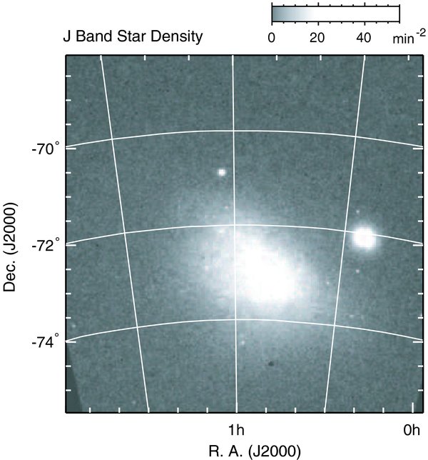
Figure 3. J-band star density map of the SMC measured using the 6X 2MASS star catalog. The map uses stars brighter than mJ = 17.5 mag.
Download figure:
Standard image High-resolution imageThe catalog is much deeper than the standard 2MASS catalog, and its limiting magnitudes vary from region to region in the SMC. For instance, a luminosity function of the stars indicates that the catalog is complete down to [mJ, mH, mK]≃[16.9,16.3,15.9] mag in the central region of the SMC, while on the outskirts the catalog is deeper and is complete down to [mJ, mH, mK] ≃ [17.5,16.9,16.3] mag.
In order to derive a color excess map, we selected stars from the catalog that satisfy the following three criteria: (1) magnitudes brighter than [mJ, mH, mK]=[18.0,17.5,17.0] mag; (2) high-quality detections, photometry, and astrometry (i.e., the read flag "rd-flg" in the catalog is either 1, 2, or 3, and the photometry flag "ph-qual" is either A, B, or C for the three bands); and (3) no counterparts among known minor planets (i.e., the minor planet flag "mp-flg" is 0).
The threshold magnitudes we used are higher than the limiting magnitude described above, but we used the above criterion (1) for constructing the color excess maps in order to increase the number of stars and to reduce noise.
For the selected stars, we applied the X percentile method described in Section 2: we placed circular cells with 2 6 diameter on a 1' grid along equatorial coordinates and calculated the colors J–H and H − KS at every 5% for X0 in the range 5 ⩽ X0 ⩽ 90% with a common X1 = 95%. The reason for adopting the 26 resolution is to compare our color excess map with the CO map newly obtained using the NANTEN telescope, which will be presented in a subsequent publication (A. Kawamura et al. 2009, in preparation).
We chose a small 15' × 25' region around the position α2000 = 0h49m40s and δ2000 = −71°57'30'' as the reference field to derive the color excess maps. This region was selected as the reference field because it is located in the outskirts of the SMC, where the H i emission is weak. In addition, the region exhibits the bluest mean star colors in the SIRIUS color excess map (described in the next subsection, see Figure 4(b)). We assume Ebg = 0 mag for this region.

Figure 4. (a) E(J − H) color excess map of the SMC measured using the 6X 2MASS star catalog. The map uses stars brighter than mJ = 18.0 and mH = 17.5 mag. (b) The same color excess map based on the SIRIUS data (Kato et al. 2007), measured using stars brighter than mJ = 18.8 and mH = 17.8 mag. The color excess maps in panels (a) and (b) are for [X0, X1] = [80, 95]% of our X percentile methods (Dobashi et al. 2008). The box drawn by the dotted line denotes the region regarded as the extinction-free reference field.
Download figure:
Standard image High-resolution imageAs an example, we display the resulting E(J − H) map in Figure 4(a), which corresponds to  in Equation (4) at X0 = 80%. In the color excess map, a faint pattern of stripes along declination with constant right ascension can be seen. This is a known systematic error in the photometry of the individual scans taken over many different nights. The effect could be avoided by using the brighter threshold magnitudes of [mJ, mH, mK] ⩽ [16.8,16.1,15.3] mag (R. Cutri 2008, private communication).
3.2. The SIRIUS Catalog
The SIRIUS catalog covers a smaller area of the SMC than the 6X 2MASS catalog, but it has a higher sensitivity; within the ∼11 deg2 coverage, ∼4.3 × 10⁵ stars are recorded in the catalog, and its 10σ limiting magnitudes are [mJ, mH, mK] = [18.8,17.8,16.6] mag.
For the SIRIUS catalog, we selected stars that satisfy the following criteria: (1) stars brighter than the above 10σ limiting magnitudes; (2) the "quality flag" representing the shape of the sources is better than "3" (c.f., "1" is the most point-like); and (3) the photometric uncertainties are smaller than 0.217 mag which corresponds to the "ph-qual" flag of C in the 6X 2MASS catalog.
We should note that there is a slight systematic error in photometry in the original SIRIUS catalog. A color map produced following Equation (1) shows a pointing-by-pointing noise pattern of a few times 0.01 mag, which is apparently due to an inappropriate flat field adopted to establish the photometry in one or more bands.
In general, photometric errors of this order are common in star catalogs, but it is not negligible in our study because dark clouds in the SMC are very faint with a color excess of only ∼0.1 mag in E(J − H) or E(H − KS). We therefore attempted to apply a correction to the catalog. For all of the stars in the catalog (i.e., not only stars in the SMC but also those in the LMC and the Bridge), we checked their (X, Y) pixel coordinates in the detector of the SIRIUS camera which counts 1024 × 1024 pixels in total (Kato et al. 2007, see their Table 2). We then calculated star colors J–H and H − KS for each star to derive the mean star color distribution as a function of (X, Y). As expected, a bumpy pattern of a few times 0.01 mag was found in the two color distributions, while a flat color distribution would be expected if the flat fields of the three bands were perfect: The mean star color J–H tends to be redder around the position (X, Y) ∼ (420, 500) and it gradually becomes bluer toward the edge of the detector. Similarly, the mean star color H − KS around the positions (X, Y) ∼ (400, 150) and ∼(400, 1000) are redder than in the outer parts of the detector. The maximum color differences between these (X, Y) positions and the edge of the detector are Δ(J − H) ∼ 0.038 mag and Δ(H − KS) ∼ 0.025 mag.
To cancel these pixel-dependent systematic errors, we attributed the errors in the J–H pixel map to the J-band photometry and those in the H − KS map to the KS band photometry, and modified the J and KS magnitudes of stars in the original SIRIUS catalog according to the flat-field correction derived above and their detector pixel coordinates (X, Y). Note that our correction should work properly only for the colors (J–H and H − KS), but not for the magnitudes (mJ, mH, and mK) of the individual stars. A new star catalog corrected for the flat-field problem is now being prepared by the authors of the original catalog, which will be available to the public in the near future (D. Kato et al. 2009, private communication).
Using the stars with thus modified photometry, we applied our X percentile method to derive the color excess maps of E(J − H) and E(H − KS) in the same way as for the 6X 2MASS data. An example of the resulting color excess map is shown in Figure 4(b). We also show the central region of the SMC in Figure 5 on a finer scale.
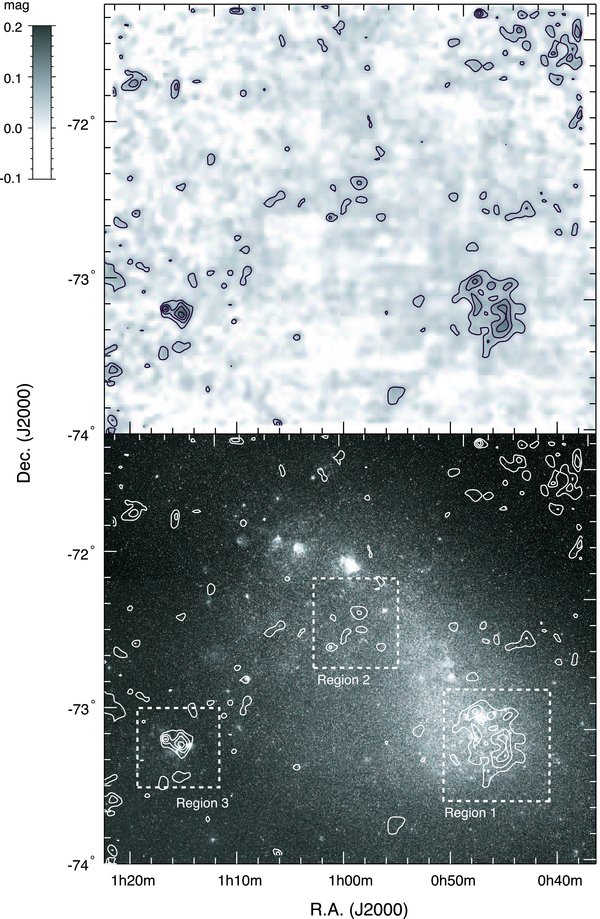
Figure 5. Color excess map of E(J − H) in Figure 4(b) shown on a finer scale, which is measured at X0 = 80% and is referred to as "E80(J − H)" in the text. The upper and lower panels show the contour map with a gray-scale and an optical image (DSS 2, red plate), respectively. The contours start from E(J − H) = 0.05 mag with a step of 0.03 mag. The grid spacing of the map is 1'. The angular resolution is 26, the same as the beam size of the CO map obtained using the NANTEN telescope (Mizuno et al. 2001). The three parts of the map indicated by the boxes with broken lines are shown in Figures 6–8.
Download figure:
Standard image High-resolution imageIn order to estimate the noise level of the color excess maps, we performed a Monte Carlo simulation. First, we composed a histogram of star colors (J–H and H − KS) found within a 15' radius around individual observed positions, and generated N stars randomly whose color distribution follows the composed color histogram. Here, N is the number of stars actually found in the 26 cells. Following Equations (1) and (2), we calculated the colors using the N stars in the same way as for the color excess maps. We repeated this simulation 100 times for each cell and regarded the standard deviation of the resulting colors as the 1σ noise level of the cells.
The noise level inferred in this manner varies from region to region mainly depending on the observed number of stars N as well as on the X0 values. In general, the noise level is lower in the central region of the SMC with larger N, and is higher in the outer regions with smaller N. For instance, in the center of the SMC, N ∼ 300 and ∼100 stars are observed for the colors J–H and H − KS, resulting in the noise levels of σ ∼ 0.01 and ∼0.008 mag over the range 30 ⩽ X0 ⩽ 80%, respectively. In external regions having N ∼ 50 and ∼15 in J–H and H − KS, respectively, the noise level for the two colors is σ ∼ 0.025 mag over the same X0 range.
In addition to the random noise described above, there may be a systematic error arising from the selection of the reference field which we set at the region indicated by the small box in Figure 4. The error would result in an offset in our final color excess maps. In Section 5.1, we attempt to analyze dark clouds detected in the color excess map by separating them into the background component (E80bg in the subsection) and the cloud component (E800). In the background component, the error should be comparable to the possible offset, while the cloud component should be much less affected. In order to determine the magnitude of the offset, we use some other regions where the mean star colors are relatively blue (e.g., top left and bottom left corners of Figure 5) as the reference field, finding that the star colors in these regions vary within a maximum uncertainty of Δ(J − H) ∼ 0.02 mag and Δ(H − KS) ∼ 0.01 mag. Our color excess maps may therefore contain an offset of this order.
We further note that there may be an additional systematic error due to the extinction by the Galactic dust lying in the foreground of the SMC. Such errors may not be removed perfectly by subtracting a simple mean star color in the reference field, if the foreground extinction varies significantly over the SMC. The Galactic component of the H i emission observed by Brüns et al. (2005) does vary over the SMC. The error, however, is likely to be much smaller than the ambiguity arising from the choice of the reference field: assuming that the standard Galactic dust-to-gas ratio AV/NH (Bohlin et al. 1978) and reddening law (Cardelli et al. 1989) of RV = 3.1 are valid for the Galactic H i emission, we estimate the error in our color excess maps to be ΔE(J − H) ∼ ΔE(H − KS) ∼ 0.003 mag at most over the region shown in Figure 5.
4. RESULTS
Although the 6X 2MASS catalog covers a much wider region around the SMC, the SIRIUS catalog corrected for the flat-field induced photometry error is deeper over the central region of the SMC where most of the known clouds are located. In addition, dark clouds are better detected in E(J − H) maps rather than E(H − KS) at the same X0 percentiles, probably due to the higher optical depth. For our study of dark clouds in the SMC, we therefore use E(J − H) maps from the SIRIUS catalog at a high percentile of X0 = 80%. Hereafter, we will call the E(J − H) map at this percentile E80(J − H) or more simply E80.
Figure 5 displays the region of the E80(J − H) map where we search for dark clouds in the SMC. The noise level of the map is σ ∼ 0.01 mag in the middle, and ∼0.04 mag in the top-right and top-left corners. In Figures 6–8, we show close-up views of three regions labeled "Region 1" to "Region 3" in Figure 5. In addition, we selected 10 clouds in the three regions by visual inspection, which are indicated as "A"–"J" in Figures 6–8. Many of these clouds have one or more counterparts among the dark clouds identified by Hodge (1974). We summarize properties of these clouds as well as their counterparts in Table 1.
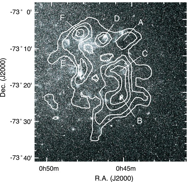
Figure 6. Close up view of Region 1 indicated in the lower panel of Figure 5. Contours start from E(J − H) = 0.05 mag with a step of 0.02 mag. Clouds found in this region are indicated by the labels "A"–"F."
Download figure:
Standard image High-resolution image
Figure 7. Same as Figure 6, but for Region 2. Clouds found in this region are indicated by the labels "G" and "H."
Download figure:
Standard image High-resolution image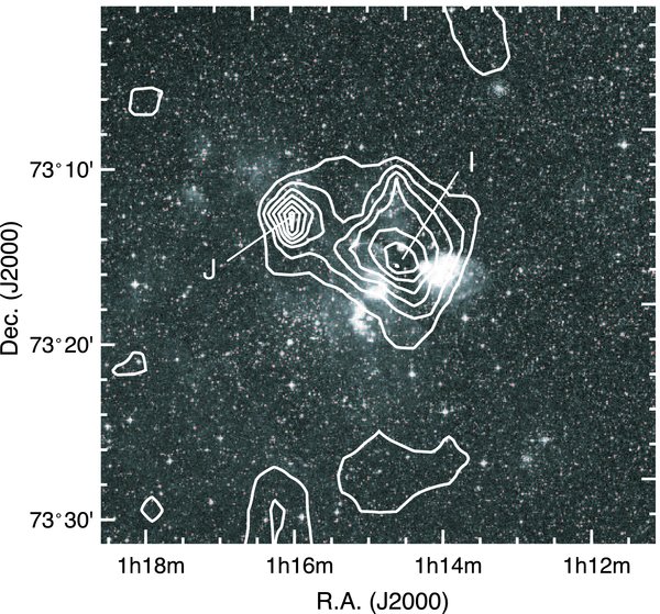
Figure 8. Same as Figure 6, but for Region 3. Clouds found in this region are indicated by the labels "I" and "J."
Download figure:
Standard image High-resolution imageTable 1. Observed Color Excess E(J − H)
| Cloud | R.A.(J2000) (h m s) | Dec.(J2000) (° ') | E80(J − H)a (mag) | Hodge (1974)b |
|---|---|---|---|---|
| A | 0 45 17 | −73 06.2 | 0.107 ± 0.011 | 1 |
| B | 0 45 20 | −73 22.2 | 0.163 ± 0.012 | 3 |
| C | 0 45 24 | −73 16.2 | 0.131 ± 0.014 | 2,4 |
| D | 0 46 40 | −73 06.5 | 0.129 ± 0.010 | 10 |
| E | 0 47 57 | −73 16.7 | 0.114 ± 0.011 | 11,12,13,14 |
| F | 0 48 17 | −73 05.8 | 0.158 ± 0.010 | 17 |
| G | 0 58 20 | −72 27.5 | 0.101 ± 0.010 | ⋅⋅⋅ |
| H | 1 01 02 | −72 41.4 | 0.177 ± 0.011 | ⋅⋅⋅ |
| I | 1 14 22 | −73 16.9 | 0.261 ± 0.027 | 45 |
| J | 1 15 42 | −73 13.4 | 0.230 ± 0.026 | ⋅⋅⋅ |
Notes.
aMeasured at X0 = 80%.
bCloud numbers given by Hodge (1974, see his Table 1 and Plate 1) whose SIMBAD nomenclature is [H74]. Right ascension (1975) of cloud number 45 corresponding to our Cloud I is denoted as 01h03  6 in his Table 1, but we believe it to be 01h13 6.
Download table as: ASCIITypeset image
It is obvious that dark clouds are well detected in the southwest part of the SMC (Region 1, see Figure 6) as well as in the outskirts, including N84 (Region 3, Figure 8). The dark clouds in these regions are also detected in CO (e.g., Mizuno et al. 2001), and their overall shapes and contrast are very similar in both the color excess and the CO maps. There are, however, some significant differences: Clouds A and C in Region 1 are very weak or not detected in CO, although they correspond to a local peak or ridge of the H i intensity map (Brüns et al. 2000, 2005), indicating that the gas is not dense enough to form molecules in these clouds. Similarly, Cloud H in Region 2 is prominent in the E80(J − H) map while there is no counterpart in CO. We should note, however, that this cloud might not be genuine due to artifacts (i.e., false stars) in the SIRIUS catalog that can be generated around bright stars (Kato et al. 2007). In fact, there is a bright star at the peak position of Cloud H (see an optical image in Figure 7).
On the other hand, CO clouds are known to exist around SMC H ii regions, including N66, which is north of Region 2 in Figure 5, and where there is no counterpart in our E80(J − H) map. We suggest that they are not detected in E80 because they are located toward the far side of the star distribution along the LOS (see Section 5.1).
Besides the good coincidence of the individual clouds in the E80(J − H) and CO maps, faint color excess is apparent in Figure 5 which extends from Region 1 to the northeast along the stellar bar. This feature is similar to the dust distribution revealed by the far-infrared dust continuum emission (Bot et al. 2004; Leroy et al. 2007), indicating that they are tracing the same diffuse dust in the SMC. In addition, there is a faint color excess extending from Region 2 to Region 3, which is similar to the H i distribution in this region connecting the main body of the SMC and the N84 region, suggesting that the faint color excess observed in the E80(J − H) map is real.
Finally, we compare the E80(J − H) map with that derived using the 6X 2MASS data at the same percentile which we call E806X(J − H) here. As seen in Figure 4, the two maps are essentially similar, though the noise level is somewhat higher in the E806X(J − H) map. Clouds A, D, and F in Region 1, as well as Cloud I in Region 3, are also well detected in the E806X(J − H) map. Cloud G in Region 2 is less evident in the E806X(J − H) map due to the higher noise level, but it is consistent within the error with its appearance in the SIRIUS map. The other clouds, however, appear much fainter, exhibiting approximately half (on average) the color excess observed in the SIRIUS map. In the southern part of Region 1, including Clouds B and C, the color excess appears especially faint. The smaller color excess in the E806X(J − H) map is probably due to the poorer sensitivity of the 6X 2MASS catalog, which is virtually complete only to [mJ, mH, mK]≃[16.9,16.3,15.9] mag in the central region of the SMC (see Section 3.1). If we apply these threshold magnitudes to derive the color excess map using the SIRIUS data, we find that the resulting map is much more similar to the E806X(J − H) map, including the southern part of Region 1.
5. DISCUSSION
5.1. Locations of Dark Clouds in the Star Distribution
In this subsection, we compare the E80(J − H) map with our model calculation to infer the cloud locations in the star distribution along the LOS.
As illustrated in Figure 1, the model parameters are: Ebg, the background color excess; ϕ(c), the distribution function of the intrinsic star colors; E0, the color excess by the cloud; Z, the cloud position; and T, the cloud thickness. Among these, we first estimate Ebg and ϕ(c) independently, and then fit the observed X0 versus  and X0 versus
  diagrams (see Figure 2) with the rest of the parameters.
In order to estimate Ebg, we attempted to separate the observed color excess E80(J − H) into background and cloud components. For this, we tentatively assumed that the regions with E80 < 0.05 mag (Figure 5) contain only the background component and the regions with E80 ⩾ 0.05 mag comprise both cloud and background components. We applied a mask to the regions with E80 ⩾ 0.05 mag and then estimated the background level in the masked regions using the IDL routine TRIGRID, and subtracted them from the original map to deduce the cloud components. In Table 2, we list the background and cloud components derived at the peak positions of the selected clouds, denoted as E80bg and E800, respectively, in the table. Note that E80bg + E800 corresponds to E80 in Table 1. The relation between E80bg and the total background Ebg is almost linear, depending on the distribution function of the intrinsic star color ϕ(c) (c = J − H in this case, see Section 3). Using ϕ(c) observed in the reference field, where we assume Ebg = 0 (see Figure 4(b)), we deduce Ebg from E80bg. The resulting Ebg values are listed in the fourth column of Table 2. Note that the inferred total background Ebg is approximately twice E80bg.
Table 2. The Best-Fitting Model Parameters
| Cloud | E80bg (mag) | E800 (mag) | Ebg (mag) | E0 (mag) | Z (%) | T (%) |
|---|---|---|---|---|---|---|
| A | 0.037 | 0.070 | 0.071 | 0.070 | 0.0 | 7.5 |
| B | 0.044 | 0.120 | 0.084 | 0.245 | 50.0 | 47.5 |
| C | 0.043 | 0.088 | 0.083 | 0.155 | 62.5 | 5.0 |
| D | 0.046 | 0.082 | 0.086 | 0.135 | 60.0 | 5.0 |
| E | 0.042 | 0.072 | 0.087 | 0.160 | 65.0 | 20.0 |
| F | 0.037 | 0.121 | 0.074 | 0.220 | 70.0 | 7.5 |
| G | 0.036 | 0.064 | 0.070 | 0.060 | 5.0 | 12.5 |
| H | 0.027 | 0.150 | 0.051 | 0.300 | 77.5 | 5.0 |
| I | 0.031 | 0.230 | 0.095 | 0.250a | 0.0a | 87.5a |
| J | 0.041 | 0.189 | 0.091 | 0.300 | 55.0 | 30.0 |
Note. aErroneous due to the poor fitting (see Figure 9).
Download table as: ASCIITypeset image
The distribution function ϕ(c) should vary slightly from region to region in the SMC, mainly depending on the population of giants and dwarfs (e.g., Bessell & Brett 1988), and can also be different inside the SMC to the reference field located in the outskirts. We therefore also attempted to derive ϕ(c) at Cloud B, the densest part in Region 1 (see Figure 6). We first measured the color distribution of stars falling within 15' of the peak position of Cloud B and then deduced ϕ(c), assuming that the distribution is reddened by the background Ebg estimated above. The derived ϕ(c) is similar to that observed in the reference field. In the following analysis, we tested both forms of ϕ(c), measured in the reference field and at Cloud B, and found that the results are in good agreement.
Using Ebg and ϕ(c) estimated in this manner, we fitted the behavior of  and
and  as a function of X0 as observed at the peak positions of Clouds A–J. In the model described in Figure 1, we set the estimated Ebg and randomly distributed 105 stars whose colors follow the ϕ(c) at Cloud B. We then calculated
  and
and  for different sets of parameters [E0, T, Z], varying E0 by 0.001 mag and T and Z by 2.5%, and compared the resulting
  and
and  with those observed to search for the set of parameters that minimize the χ2. Results are shown in Figure 9. We summarize the best model parameters [E0, T, Z] in Table 2.
Figure 9. Sample of  (open circles) and
  (filled circles) as a function of X0 measured at the peak positions of Clouds "A"–"J" in Figures 6–8 with a common X1 of 95%. The solid lines denote the best-fitting model values calculated with the parameter [E0, T, Z] shown in the parentheses in each panel in this order.
Download figure:
Standard image High-resolution imageIn Figure 9, the  and
and  diagrams at Clouds A and G are flat, indicating that the clouds at these positions are located almost in front of the star distribution in the SMC and should be completely detected in our E80 map. On the other hand, the diagrams at Clouds I and J in Region 3 are rather complex. In particular, the diagram measured at Cloud I cannot be fitted by our simple model. This is most likely due to two or more cloud components lying on the same LOS, which is not taken into account in our model. In fact, it is interesting to note that recent CO observations made with the NANTEN telescope have revealed two distinct velocity components toward Cloud I: one is a component at VLSR = 160 km s−1 extending over the cloud surface, and the other is a weak component at VLSR = 150 km s−1 detected only around the peak position of Cloud I (A. Kawamura et al. 2009, in preparation).
For the other clouds, the diagrams increase with X0 and some of them show concave  curves, which is a characteristic feature of clouds whose far sides are located toward the back of the star distribution (i.e., Z + T>50%, see Figure 2(c)). The color excess of such clouds can be highly underestimated in our E80 map. In fact, a comparison with the model calculations indicates that our values of E800 underestimate E0 by a factor of ∼2 (see Table 2).
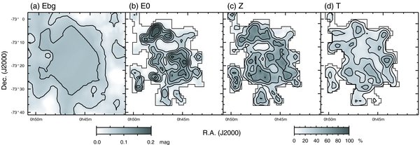
We applied the above fitting procedure to the regions with E80 ⩾ 0.05 mag in Region 1 to estimate how much we may underestimate the true color excess in our E80 map. The resulting E0 map is shown in Figure 10, together with Z, T, and Ebg maps. Although the overall distribution of the E0 is similar to that of E80 map, we found that E0 is larger than E800 by a factor of ∼2 on average, as expected. In addition, contrasts of the clouds are different in the E0 map, depending on the cloud parameters Z and T. For example, the color excess at Cloud A is unchanged and remains E800 = E0=0.07 mag because it is located at Z ∼ 0 (Figure 10(b) and (c)). On the other hand, the color excess measured at Cloud F, which has larger Z, increases by a factor of 1.8 from E800=0.121 mag to E0=0.220 mag (see Table 2), indicating that Cloud F is about twice as dense as observed in the E80 map.
Figure 10. Panel (a) shows the background color excess Ebg in Region 1 inferred from the E80(J − H) maps measured at various X0 based on Equation (4). The other panels (b), (c), and (d) show the distributions of the model parameters—E0, Z, and T—best fitting the observed data (see Figure 1). Contours are drawn at every 0.03 mag starting from E(J − H) = 0.05 mag in panels (a) and (b), and at every 20% starting from Z = 20% in panel (c), and at every 10% starting from T = 10% in panel (d). Thin solid lines in panels (b)–(d) represent the area where we performed the fitting by the model.
Download figure:
Standard image High-resolution image
To conclude, both the background and cloud components observed in our E80(J − H) map are likely to underestimate the true color excess by a factor of ∼2 on average. However, the error (∼2) is rather uncertain, because the cloud parameter maps in Figure 10 are still tentative and may be erroneous. This is because it is difficult to determine the model parameters E0, Z, and T that minimize χ2 in the case of clouds with Z + T>50% showing concave  curves. In general, E0 tends to be overestimated for such
  curves, and the error in E0 is larger for clouds with fainter color excess (e.g., E80 < 0.05 mag). Our E0 map can therefore be regarded as the upper limit to the actual E0 values, while E800 should be considered as a lower limit.
5.2. Dust-to-Gas Ratio in the SMC
As seen in Figure 9, clouds in Region 1 have rather simple  and
and  curves and are fitted well by our model. Four of them, Clouds B, D, E, and F, are also well detected in CO using the NANTEN telescope and their virial masses MVIR have been estimated by Mizuno et al. (2001, see their Figure 4) as MVIR ∝ R(ΔV)2, where R and ΔV are the cloud radius and the observed CO line width. We compare the virial masses with our E(J − H) data to derive the dust-to-gas ratio AV/NH of these clouds, which can be expressed as,
where ∫E(J − H)ds is the color excess integrated over the cloud surface, and α is a coefficient. We assume the cloud surface to be the area defined by the lowest contours (0.45 K km s−1) in the velocity-integrated CO map presented by Mizuno et al. (2001, see their Figure 3). The coefficient α is taken to be 2.67 × 10⁻²²mag H-1 cm2, assuming the relation AV = 10.9E(J − H) that is derived from the reddening law determined by Cardelli et al. (1989) for RV = 3.1. We note that the reddening law in the SMC is known to be similar to that in the MW in the VIS to near-infrared wavelengths, despite their significant difference in the ultraviolet (Gordon et al. 2003). Moreover, it was recently found by Zagury (2007) that the extinction curves in the SMC, MW, and LMC obey the same reddening law, similar to that found by Cardelli et al. (1989).
For E(J − H) in Equation (5), we used the values of the cloud components (E800 and E0) described in the previous subsection, since CO emission is expected to arise from the dense clouds but not from the diffuse background components (E80bg and Ebg). Resulting values of AV/NH for the individual clouds are summarized in Table 3, as well as the surface areas and virial masses measured by Mizuno et al. (2001). The minimum estimate of AV/NH based on E800 varies around ∼1 × 10⁻²²mag H-1 cm2, and the maximum estimate using E0 ranges from ∼2 ×10⁻²² to ∼ 3 ×10⁻²² mag H-1 cm2. The mean value of the four clouds, weighted by MVIR, is ∼1.5 ×10⁻²², which is about a half the value of AV/NH measured using the same method for the clouds near the 30 Dor region in the LMC (e.g., ∼3×10⁻²² for LMC-154; Dobashi et al. 2008), and about one third of the standard Galactic value (5.34 × 10⁻²² for RV = 3.1; Bohlin et al. 1978). Our average value of AV/NH is about twice the value measured for a limited number of sightlines in the SMC by Gordon et al. (2003, 7.59 × 10⁻²³), which is closer to our lower limit (∼1×10⁻²²). We should note that the AV/NH value measured by Gordon et al. takes into account only the neutral hydrogen (H i) but not hydrogen molecules (H2), which may increase the difference between their and our estimates for AV/NH. The effect should be small, however, since the total extinction toward their sample stars is rather low (E(B − V) ≲ 0.2 mag) and therefore H2 may not be abundant along the LOS toward their sample stars.
Table 3. Dust-to-Gas Ratio of the Selected Clouds in the SMC
| Cloud | Areaa (arcmin2) | MaVIR (105 M☉) | ∫E800ds (mag arcmin2) | ∫E0ds (mag arcmin2) | AV/NH b (10−22 mag H-1 cm2) |
|---|---|---|---|---|---|
| B | 69 | 9.3 | 3.68 | 7.85 | 1.1–2.3 (1.7 ± 0.6) |
| D | 18 | 1.7 | 0.78 | 2.12 | 1.2–3.3 (2.3 ± 1.1) |
| E | 40 | 5.6 | 1.56 | 3.55 | 0.7–1.7 (1.2 ± 0.5) |
| F | 13 | 3.1 | 0.96 | 2.07 | 0.8–1.8 (1.3 ± 0.5) |
Notes. aMeasured in CO (Mizuno et al. 2001). bMinimum–maximum estimates (see the text). The mean value is given in the parentheses.
Download table as: ASCIITypeset image
Instead, we think that the difference between our value of AV/NH and the value determined by Gordon et al. is probably due to the variations of AV/NH within the SMC. Variations in AV/NH of a factor of ∼2 are observed also among clouds in the LMC (Dobashi et al. 2008; Bernard et al. 2008) and among the Galactic clouds within 1 kpc from the Sun (F. Egusa et al. 2009, in preparation). In addition, the rather large uncertainty in our analysis (see Section 5.1) may also be responsible for the difference. However, it is also worth noting that the virial mass derived as MVIR ∝ R(ΔV)2 (Mizuno et al. 2001) may underestimate the true cloud mass by a factor of ∼2 in the case of giant molecular clouds in the SMC, not only because of the ambiguity in determining the cloud radius but also because of possible cloud support by the magnetic field (Bot et al. 2007). If this is the case for the MVIR values that we adopted in our analysis, then our estimate for AV/NH is very close to that found by Gordon et al.
6. SUMMARY
We have carried out a survey for dark clouds in the SMC based on the near-infrared color excess map that we constructed from the SIRIUS catalog. The main conclusions of this paper can be summarized as follows:
- 1.Applying the X percentile method to the SIRIUS star catalog presented by Kato et al. (2007), we have derived a color excess map of E(J − H) that reveals the distributions of dark clouds and the diffuse background in the SMC.
- 2.We selected 10 dark clouds (Clouds A–J) based on the E(J − H) map. The apparent color excess of these clouds measured at X0 = 80% ranges from E(J − H)=0.10 to 0.26 mag at 26 resolution, and their shapes and contrasts are similar to that revealed by the CO observations carried out with the NANTEN telescope at the same angular resolution (Mizuno et al. 2001).
- 3.Comparison with model calculations indicates that many of the selected clouds (except Clouds A and G) are likely to be located at or extending toward the far side of the star distributions in the SMC along the LOS, in which case the apparent color excess may underestimate the true color excess by a factor of ∼2. We attempted to fit the observed E(J − H) map to infer the distributions of the true color excess.
- 4.Comparison of the E(J − H) map derived in this paper with the CO map presented by Mizuno et al. (2001) allows us to estimate the dust-to-gas ratio, AV/NH. Using the virial mass derived by Mizuno et al., we find that the AV/NH ratio in the SMC varies from cloud to cloud within the range 1–2 × 10⁻²² mag H-1 cm2, with a mean mass-weighted value of ∼1.5 × 10⁻²² mag H-1 cm2. If the virial mass that we adopted underestimates the true cloud mass by a factor of ∼2 as suggested by Bot et al. (2007), the mean value would decrease to ∼0.8 × 10⁻²² mag H-1 cm2, which is consistent with that previously reported by Gordon et al. (2003).
We are grateful to D. Kato and R. Cutri for their useful advice regarding the SIRIUS and 6X 2MASS star catalogs. This work was financially supported by Ito Science Society (H19), as well as by Yamada Science Foundation for the promotion of the natural sciences (2008-1125). This publication makes use of data products from the Two Micron All Sky Survey, which is a joint project of the University of Massachusetts and the Infrared Processing and Analysis Center/California Institute of Technology, funded by the National Aeronautics and Space Administration and the National Science Foundation.