WASP-47: A HOT JUPITER SYSTEM WITH TWO ADDITIONAL PLANETS DISCOVERED BY K2

Due to their large sizes and short orbital periods, hot Jupiters (roughly Jupiter-mass planets with periods between 0.8 and 6.3 days; Steffen et al. 2012) are among the easiest exoplanets to detect. Both the first exoplanet discovered around a main sequence star (Mayor & Queloz 1995) and the first known transiting exoplanet (Charbonneau et al. 2000; Henry et al. 2000) were hot Jupiters. Until the launch of the Kepler space telescope in 2009, the majority of known transiting exoplanets were hot Jupiters. Hot Jupiters allow for the determination of many planetary properties, including their core masses (Batygin et al. 2009) and atmospheres (Charbonneau et al. 2002). For these reasons, transiting hot Jupiters were and continue to be the subject of many follow-up studies (Kreidberg et al. 2014).

One such follow-up study is the search for additional planets in the system revealed by small departures from perfect periodicity in the hot Jupiter transit times (called transit timing variations or TTVs). TTVs were predicted (Agol et al. 2005; Holman & Murray 2005) and searched for (Steffen & Agol 2005; Gibson et al. 2009), but very little evidence for TTVs was found until the Kepler mission discovered smaller transiting planets on longer period orbits than the hot Jupiters detected from the ground (Holman et al. 2010; Lissauer et al. 2011).

The lack of TTVs for hot Jupiters implies a dearth of nearby planets in these systems. While systems exist with a known hot Jupiter and a distant (≳200-day period) companion (Endl et al. 2014; Knutson et al. 2014) or a warm Jupiter (orbital period 6.3–15.8 days) and a close-in planet (for example, KOI 191: Steffen et al. 2010; Sanchis-Ojeda et al. 2014), searches for close-in, companions to hot Jupiters (as in Steffen et al. 2012) have not yet been successful.

This apparent scarcity supports the idea that hot Jupiters form beyond the ice line and migrate inwards via high eccentricity migration (HEM), a process which would destabilize the orbits of short-period companions (Mustill et al. 2015). Studies of the Rossiter–McLaughlin effect have also found the fingerprints of HEM (Albrecht et al. 2012). However, statistical work has shown that not all hot Jupiters can form in this way (Dawson et al. 2015), so some hot Jupiters may have close-in planets. Additionally, HEM may not exclude nearby, small planets (Fogg & Nelson 2007).

In this paper, we present an analysis of the WASP-47 system (originally announced by Hellier et al. 2012) that was recently observed by the Kepler Space Telescope in its new K2 operating mode (Howell et al. 2014). In addition to the previously known hot Jupiter in a 4.16-day orbit, the K2 data reveal two more transiting planets: a super-Earth in a 19-hr orbit, and a Neptune-sized planet in a 9-day orbit. We process the K2 data, determine the planetary properties, and measure the transit times of the three planets. We find that the measured TTVs are consistent with the theoretical TTVs expected from this system and measure or place limits on the planets' masses. Finally, we perform many dynamical simulations of the WASP-47 system to assess its stability.

Kepler observed K2 Field 3 for 69 days between 2014 November 14 and 2015 January 23. After the data were publicly released, one of us (HMS) identified additional transits by visual inspection of the Pre-search Data Conditioned light curve of WASP-47 (designated EPIC 206103150) produced by the Kepler/K2 pipeline. We confirmed the additional transits by analyzing the K2 pixel level data following Vanderburg & Johnson (2014). A Box-Least-Squares (Kovács et al. 2002) periodogram search (as implemented in Muirhead et al. 2015) of the processed long cadence light curve identified the 4.16-day period hot Jupiter (WASP-47 b), a Neptune sized planet in a 9.03-day period (WASP-47 d), and a super-Earth in a 0.79-day period (WASP-47 e).

Because of the previously known hot Jupiter, WASP-47 was observed in K2's "short cadence" mode, which consists of 58.3 s integrations in addition to the standard 29.41 minute "long cadence" integrations. K2 data are dominated by systematic effects caused by the spacecraft's unstable pointing which must be removed in order to produce high quality photometry. We began processing the short cadence data following Vanderburg & Johnson (2014) to estimate the correlation between K2's pointing and the measured flux (which we refer to as the K2 flat field). We used the resulting light curve and measured flat field as starting points in a simultaneous fit of the three transit signals, the flat field, and long term photometric variations (following Vanderburg et al. 2015). The three planetary transits were fit with Mandel & Agol (2002) transit models, the flat field was modeled with a spline in Kepler's pointing position with knots placed roughly every 0.25 arcsec, and the long term variations were modeled with a spline in time with knots placed roughly every 0.75 days. We performed the fit using the Levenberg–Marquardt least squares minimization algorithm (Markwardt 2009). The resulting light curve⁷ shows no evidence for K2 pointing systematics, and yielded a photometric precision of 350 parts per million (ppm) per 1 minute exposure. For comparison, during its original mission, Kepler also achieved 350 ppm per 1 minute exposure on the equally bright (Kp = 11.7) KOI 279.

We measured planetary and orbital properties by fitting the short cadence transit light curves of all three planets with Mandel & Agol (2002) transit models using Markov Chain Monte Carlo (MCMC) algorithm with affine invariant sampling (Goodman & Weare 2010). We used 50 walkers and 9000 links, and confirmed convergence with the test of Geweke (1992) and a comparison of the Gelman–Rubin statistics for each parameter. 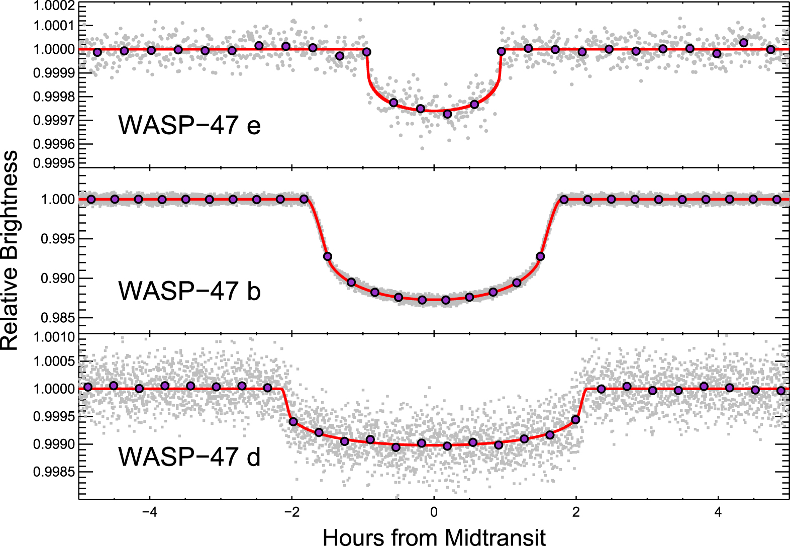We fit for the q₁ and q₂ limb darkening parameters from Kipping (2013), and for each planet, we fit for the orbital period, time of transit, orbital inclination, scaled semimajor axis $a/{R}_{\star },$ and ${R}_{p}/{R}_{\star }.$ Our best-fit model is shown in Figure 1 and our best-fit parameters are given in Table 1. Our measured planetary parameters for WASP-47 b are consistent with those reported in Hellier et al. (2012).

Zoom In Zoom Out Reset image size

Table 1.  System Parameters for WASP-47

Parameter	Value		68.3% Confidence	Comment
			Interval Width
Stellar Parameters
R.A.	22:04:48.7	⋯	⋯	⋯
Decl.	−12:01:08	⋯	⋯	⋯
M⋆ (M⊙)	1.04	±	$0.08$	A
R⋆ (R⊙)	1.15	±	$0.04$	A
Limb darkening q1	0.399	±	$0.020$	B, D
Limb darkening q2	0.420	±	$0.018$	B, D
$\mathrm{log}{g}_{\star }$ (cgs)	4.34	±	$0.01$	A
[M/H]	$+0.36$	±	$0.05$	A
Teff (K)	5576	±	$67$	A
${e}_{d}\mathrm{cos}{\omega }_{d}-{e}_{b}\mathrm{cos}{\omega }_{b}$	-0.0002	±	0.0195	A, B, C
${e}_{d}\mathrm{sin}{\omega }_{d}-{e}_{b}\mathrm{sin}{\omega }_{b}$	0.0039	±	0.0179	A, B, C
WASP-47 b
Orbital Period, P (days)	4.1591287	±	$0.0000049$	B
Radius Ratio, $({R}_{P}/{R}_{\star })$	0.10186	±	$0.00023$	B
Scaled semimajor axis, a/R⋆	9.715	±	$0.050$	B
Orbital inclination, i (deg)	89.03	±	$0.27$	B
Transit impact parameter, b	0.164	±	$0.045$	B
Time of Transit tt (BJD)	2457007.932131	±	0.000023	B
TTV amplitude (minutes)	0.63	±	0.10	B
MP (M⊕)	341		${}_{-55}^{+73}$	A, B, C
RP (R⊕)	12.77	±	$0.44$	A, B
WASP-47 e
Orbital Period, P (days)	0.789597	±	$0.000013$	B
Radius Ratio, $({R}_{P}/{R}_{\star })$	0.01456	±	$0.00024$	B
Scaled semimajor axis, a/R⋆	3.24	±	$0.14$	B
Orbital inclination, i (deg)	87.0	±	$3.1$	B
Transit impact parameter, b	0.17	±	$0.15$	B
Time of Transit tt (BJD)	2457011.34849	±	0.00038	B
TTV amplitude (minutes)	<1.2 min for any TTV period <80 days			B
MP (M⊕)	<22		95% Confidence	C
RP (R⊕)	1.829	±	$0.070$	A, B
WASP-47 d
Orbital Period, P (days)	9.03081	±	$0.00019$	B
Radius Ratio, $({R}_{P}/{R}_{\star })$	0.02886	±	$0.00047$	B
Scaled semimajor axis, a/R⋆	16.33	±	$0.87$	B
Orbital inclination, i (deg)	89.36	±	$0.67$	B
Transit impact parameter, b	0.18	±	$0.16$	B
Time of Transit tt (BJD)	2457006.36927	±	0.00044	B
TTV amplitude (minutes)	7.3	±	1.9	B
MP (M⊕)	15.2		± 7	C
RP (R⊕)	3.63	±	$0.14$	A, B

Notes. A: Parameters come from Mortier et al. (2013). B: Parameters come from analysis of the K2 light curve. C: Parameters come from dynamical fits to the observed transit timing variations. D: We report the magnitude of the impact parameter, whereas the true value could be positive or negative.

Download table as:  ASCIITypeset image

We also fitted for the transit times and transit shapes of each transit event in the short cadence light curve simultaneously (due to the relatively short orbital periods sometimes causing two transits to overlap) using MCMC. Our measured transit times⁸ are shown in Figure 2. We find that the TTVs of WASP-47 b and WASP-47 d are detected at high significance. The two TTV curves are anti-correlated and show variations on a timescale of roughly 50 days. This is consistent with the TTV super-period we expect for planets orbiting in this configuration, which we calculate to be P_TTV = 52.67 days using Equation (7) of Lithwick et al. (2012).

Zoom In Zoom Out Reset image size

Transiting planet signals like those we find for WASP-47 e and WASP-47 d can be mimicked by a variety of astrophysical false positive scenarios. In this section, we argue that this is unlikely in the case of the WASP-47 system. The hot Jupiter, WASP-47 b, was discovered by Hellier et al. (2012) and confirmed with radial velocity (RV) follow-up, which showed no evidence for stellar mass companions or spectral line shape variations, and detected the spectroscopic orbit of the planet. In the K2 data, we detect TTVs of WASP-47 b which are anti-correlated with the TTVs of WASP-47 d, and which have a super-period consistent with what we expect if both of these objects are planets. The TTVs therefore confirm that WASP-47 d is a planet in the same system as WASP-47 b. We also fitted the transit durations with a power law and found that they followed the expected P^1/3 relation (when P is orbital period) for planets orbiting a single star.

The light curve is not of sufficiently high quality to detect TTVs for the smaller WASP-47 e, so we validate its planetary status statistically. We do this using vespa (Morton 2015), an implementation of the procedure described in Morton (2012). Given constraints on background sources which could be the source of the transits, a constraint on the depth of any secondary eclipse, the host star's parameters and location in the sky, and the shape of the transit light curve, vespa calculates the probability of a given transit signal being an astrophysical false positive. Both visual inspection of archival imaging and a lucky imaging search (Wöllert et al. 2015) found no close companions near WASP-47, but the lucky imaging is not deep enough to rule out background objects that could cause the shallow transits of WASP-47 e. Following Montet et al. (2015), we define a conservative radius inside of which background sources could cause the transits. We adopt a radius of 12 arcsec; we detect the transits with photometric apertures as small as 6 arcsec in radius and allow for the possibility that stars outside of the aperture could contribute flux due to Kepler's 6 arcsec point-spread function. We find that WASP-47 e has a false positive probability (FPP) of roughly 5 × 10⁻⁴. We find using the expressions from Lissauer et al. (2012) that since this is a three-planet system, its FPP decreases to less than 10⁻⁵. As such, we consider WASP-47 e to be validated as a bona fide planet.

4.1. Stability Analysis

We test the dynamical stability of the WASP-47 planetary system with a large ensemble of numerical simulations. The K2 data determine the orbital periods of the three bodies to high precision and place constraints on the other orbital elements. We sample the allowed ranges of the orbital elements for all three planets, randomizing the orbital phases of the three bodies. We assigned masses by sampling the distribution of Wolfgang et al. (2015) for the measured planet radii. We chose eccentricities from a uniform distribution that extends up to e = 0.3. We discard systems that do not satisfy the stability criteria enumerated in Fabrycky et al. (2014).

Given a set of 1000 such initial conditions, we numerically integrate the systems using the Mercury6 integration package (Chambers 1999). We use a Bulirsch–Stoer (B–S) integrator, requiring that system energy be conserved to 1 part in 10⁹. We integrate the system for a total simulation length of 10 Myr, unless the system goes unstable on a shorter timescale due to ejection of a planet, planetary collisions, or accretion of a planet by the central star. To perform these computationally intensive simulations, we use the Open Science Grid (OSG; Pordes et al. 2007) accessed through XSEDE (Towns et al. 2014).

The results from this numerical survey are shown in Figure 3. The left panel shows the fraction of systems remaining stable as a function of time. About 30% of the systems are unstable over short timescales, and almost 90% of the systems are unstable over long timescales. Once the systems reach ages of ∼10⁴ years, they tend to survive over the next three orders of magnitude in integration time. The remaining three panels show the mass and initial eccentricity of the three planets, sampled from the distributions specified above. One clear trend is that low eccentricity systems tend to survive, whereas systems with e_p > 0.05 are generally unstable. A second trend that emerges from this study is that stability does not depend sensitively on the planet masses (provided that the orbits are nearly circular). Stable systems arise over a wide range of planet masses, essentially the entire range of masses allowed given the measured planetary radii.

Zoom In Zoom Out Reset image size

WASP-47 b and WASP-47 d orbit within about 20% of the 2:1 mean motion resonance (MMR). For completeness, we carried out a series of numerical integrations where the system parameters varied over the allowed, stable range described above. In all trials considered, the resonance angles were found to be circulating rather than librating, so there is no indication that the system resides in MMR.

Each of the numerical integrations considered here spans 10 Myr, which corresponds to nearly one billion orbits of the inner planet. Tidal interactions occur on longer timescales than this and should be considered in future work. In particular, the survival of the inner super-Earth planet over the estimated lifetime of the WASP-47 system could place limits on the values of the tidal quality parameters Q for the bodies in the system.

4.2. Theoretical TTVs

We performed a second ensemble of numerical simulations to estimate the magnitude of TTVs in the WASP-47 system. We used initial conditions similar to those adopted in the previous section, but with starting eccentricities e < 0.1.

We integrated each realization of the planetary system for 10 years using the Mercury6 B–S integrator with time-steps <0.5 s. We extracted transit times from each integration for each planet, resulting in theoretical TTV curves. The resulting distributions of predicted TTV amplitudes are shown in Figure 4. The three distributions have approximately the same shape and exhibit well defined peaks. The TTV amplitudes we measured in Section 2 are consistent with the distributions we produced theoretically.

Zoom In Zoom Out Reset image size

4.3. Mass Measurements from the TTVs

We measure the TTVs with high enough precision that dynamical fits can give estimates of the planetary masses. We use TTVFAST (Deck et al. 2014) to generate model transit times for each observed epoch for each planet, and use emcee (Foreman-Mackey et al. 2013), an MCMC algorithm with affine invariant sampling, to minimize residuals between the observed TTVs and these model TTVs. In these fits, we allow each planet's mass, eccentricity, argument of pericenter, and time of first transit to float. We imposed a uniform prior on eccentricity between 0 and 0.06 (as required for long-term stability). We initialized the chains with random arguments of pericenter and masses drawn from the Hellier et al. (2012) mass posterior for WASP-47 b and the distribution of Wolfgang et al. (2015) for WASP-47 e and WASP-47 d. We used 64 walkers and 20,000 iterations to explore the parameter space, and discarded the first 2500 iterations as "burn-in." We confirmed that the MCMC chains had converged using the test of Geweke (1992) and the Gelman–Rubin statistics (which were below 1.05 for every parameter). The best-fit model points are overlaid with the observed TTVs for the outer two planets in Figure 5.

Zoom In Zoom Out Reset image size

We find that we are able to measure the masses of WASP-47 b and WASP-47 d and place an upper limit on the mass of WASP-47 e. We additionally provide limits on the quantities ${e}_{c}\mathrm{cos}{\omega }_{c}-{e}_{b}\mathrm{cos}{\omega }_{b}.$ These masses and limits are summarized in Table 1. We measure a mass of 341${}_{-55}^{+73}$ M_⨁ for WASP-47 b, which is consistent with the mass measured by Hellier et al. (2012) of 362 ± 16 M_⨁ at the 1-σ level. The mass of WASP-47 d is 15.2 ± 7 M_⨁. Only an upper limit can be placed on WASP-47 e of <22 M_⨁.

WASP-47 is unusual: it is the first hot Jupiter discovered to have additional, close-in companion planets. Using the Exoplanet Orbit Database (Han et al. 2014), we found that among the 224 systems containing a planet with mass greater than 80 M_⨁ and orbital period less than 10 days, only six contain additional planets, and none of them have additional planets in orbital periods shorter than 100 days. That the additional planets in the WASP-47 system are coplanar with the hot Jupiter and that the planets are unstable with e ≳ 0.05 implies that the WASP-47 planets either migrated in a disk or some damping near the end of migration took place to bring them into their present compact architecture.

The continued existence of the companions in this system indicates that HEM cannot serve as the sole formation mechanism for hot Jupiters. HEM would likely have disrupted the orbits of the smaller planets. It is quite possible that there is more than one potential formation mechanism for hot Jupiters. Additionally, recent observations have identified an additional Jupiter-mass planet in a 571-day orbit (called WASP-47c; Neveu-VanMalle et al. 2015) in this system, making this the first hot Jupiter with both close-in companions and an external perturber. Future dynamical work will place limits on the architecture of this system.

WASP-47 is a rare system for which planet masses can be determined using TTVs measured from the K2 data set. This is because (a) the planets are far enough away from resonance that the super-period (52.7 days) is shorter than the K2 observing baseline (69 days), and (b) the planets are massive enough that the TTVs are large enough to be detectable. The detection of TTVs was also aided by the fact that WASP-47 was observed in short cadence mode, which is unusual for K2.

Finally, WASP-47 is a favorable target for future follow-up observations. The V-band magnitude is 11.9, bright enough for precision RV follow-up studies. The K2 light curve shows no evidence for rotational modulation, indicating that WASP-47 is photometrically quiet and should have little RV jitter. Measuring the mass of the two planetary companions with RVs could both improve the precision of the inferred masses and test the consistency of TTV and RV masses, between which there is some tension (e.g., KOI 94: Masuda et al. 2013; Weiss et al. 2013). The 1.3% depth of the transits of WASP-47 b makes it easily detectable from the ground. Previous ground based searches for TTVs of hot Jupiters have attained timing uncertainties of ∼20 s, lower than the measured TTV amplitude for WASP-47 b (Gibson et al. 2009). Follow-up transit observations could place additional constraints on the masses of the WASP-47 planets.

In this work we have studied the WASP-47 planetary system by using data from the Kepler/K2 mission along with supporting theoretical calculations. Our main results can be summarized as follows.

• 1.  
  In addition to the previously known hot Jupiter companion WASP-47 b, the system contains two additional planets that are observed in transit. The inner planet has a ultra-short period of only 0.789597 days, and radius of 1.829 R_⨁. The outer planet has a period of 9.03081 days and a radius of 3.63 R_⨁, comparable to Neptune.
• 2.  
  The system is dynamically stable. We have run 1000 10 Myr numerical integrations of the system. The planetary system remains stable for the 10% of the simulations that start with the lowest orbital eccentricities.
• 3.  
  The particular planetary system architecture of WASP-47 results in measurable TTVs, which are in good agreement with the TTVs we find from numerical integrations of the system. We use the TTVs to measure the masses of WASP-47 b (consistent with RV measurements) and WASP-47 d.
• 4.  
  This compact set of planets in nearly circular, coplanar orbits demonstrates that at least a subset of Jupiter-size planets can migrate in close to their host star in a dynamically quiet manner, suggesting that there may be more than one migration mechanism for hot Jupiters.

The WASP-47 planetary system provides a rare opportunity where planets can be both inferred from TTVs and seen in transit. Future observations comparing the system parameters inferred from TTVs with those inferred from RVs will qualitatively test TTVs as a general technique.

We are grateful to Kat Deck and Tim Morton for significant assistance. We thank Marion Neveu-VanMalle, Eric Bell, Moiya McTier, Mark Omohundro, and Alexander Venner for useful conversations. We thank John Johnson for his guidance and the anonymous referee for their very useful comments. We acknowledge the Planet Hunters team for its community. This work used the Extreme Science and Engineering Discovery Environment (NSF ACI-1053575) and the OSG (NSF, DoE). J.B. and A.V. are supported by the NSF GRFP (DGE 1256260, DGE 1144152). This research has used the Exoplanet Data Explorer at http://www.exoplanets.org. The data in this paper were obtained from the Mikulski Archive for Space Telescopes. This paper includes data collected by the Kepler/K2 mission (funding provided by the NASA Science Mission directorate), and we gratefully acknowledge the efforts of the entire Kepler/K2 team.

Facility: Kepler/K2 - The Kepler Mission.