
Abstract
Northern hemisphere winter 2009/10 was exceptional for atmospheric circulation: the North Atlantic Oscillation (NAO) index was the lowest on record for over a century. This contributed to cold conditions over large areas of Eurasia and North America. Here we use two versions of the Met Office GloSea4 seasonal forecast system to investigate the predictability of this exceptional winter. The first is the then operational version of GloSea4, which uses a low top model and successfully predicted a negative NAO in forecasts produced in September, October and November 2009. The second uses a new high top model, which better simulates sudden stratospheric warmings (SSWs). This is particularly relevant for 2009/10 due to its unusual combination of a strong El Niño and an easterly quasi-biennial oscillation (QBO) phase, favouring SSW development. SSWs are shown to play an influential role in surface conditions, producing a stronger sea level pressure signal and improving predictions of the 2009/10 winter.
Export citation and abstract BibTeX RIS

Content from this work may be used under the terms of the Creative Commons Attribution-NonCommercial-ShareAlike 3.0 licence. Any further distribution of this work must maintain attribution to the author(s) and the title of the work, journal citation and DOI.
1. Introduction
Northern hemisphere winter 2009/10 circulation was extreme, with record low Arctic Oscillation (AO) and NAO indices [1, 2]. The circulation was an important driver of low temperatures over large areas of Eurasia and North America [2, 3], although northern hemisphere mean temperatures taken from e.g. HadCRUT3 ([4], www.hadobs.org) or GISTEMP ([5], http://data.giss.nasa.gov/gistemp) were still above the long term mean. An obvious question to ask is to what extent this event was predictable.
Several proposed mechanisms suggest predictability of winter climate based on conditions in preceding months [6]. These include Arctic sea ice anomalies affecting the atmosphere through low-level heating [7]; atmospheric preconditioning, involving autumn AO persistence into winter [8]; and forcing of the NAO by an Atlantic tripole sea surface temperature (SST) pattern [9].
Previous work has also shown links between tropospheric and stratospheric circulation, with sudden stratospheric warmings (SSWs) generating a downward propagating signal that influences tropospheric circulation in late winter [10, 11]. Modelling of SSWs and their surface impacts may therefore offer the potential for improved predictability of winter climate [12]. A minor SSW occurred in early December 2009 and a major SSW in late January, with each SSW preceding cold surface conditions [13]. Eurasian snow cover anomalies have been proposed as a source of tropospheric forcing of the stratosphere, leading to enhanced likelihood of such SSWs [14].
Here we investigate winter 2009/10 with the Met Office seasonal forecast system GloSea4 [15] in both the operational configuration then being used (low top) and the subsequent operational configuration using a model with an extended vertical domain and more levels (high top). First we examine the low top model results, and investigate whether they can be explained by existing hypotheses. The high top model better resolves the stratosphere and simulates SSWs, so may be expected to give better results. We assess the performance of the high top model and compare it with the low top model; we also examine whether the high top model reproduces previously identified links between stratospheric and tropospheric circulation.
2. Data and methods
Two configurations of the GloSea4 system are used, both based on the HadGEM3 coupled ocean–atmosphere model [16] with an atmospheric horizontal resolution of 1.875° longitude by 1.25° latitude. Forecasts are initialized with atmosphere, land surface and ocean data from operational Met Office analyses. These analyses are not available for the full hindcast period, so hindcasts (used to generate a model climatology to correct systematic forecast biases) are initialized with ERA-Interim reanalysis data from ECMWF and ocean data from satellite and in situ datasets. GloSea4 uses a lagged approach to represent the uncertainty in initial conditions. For more details see [15].
The low top (L38) and high top (L85) model configurations have 38 and 85 vertical levels, with top-level heights of 40 km and 85 km respectively. The operational GloSea4 system in use during the 2009/10 winter produced regular forecasts before and throughout the winter. We compare L38 and L85 forecasts initialized between 25 October and 9 November to analyse the months December to February (DJF).
For L38, the operational GloSea4 system produced 33 forecasts for 2009/10 and 118 hindcasts for the period 1989–2002; our L85 reruns comprise 39 forecasts for 2009/10 and 122 hindcasts for the period 1992–2005. (Different hindcast periods are used at L38 and L85 due to an update in the GloSea4 system. Rather than focus on the hindcast years common to L38 and L85 we chose to retain all the years for a better climatology estimate.) Observed mean sea level pressure (MSLP) fields are taken from the HadSLP2r dataset [17], with 200 hPa geopotential height from NCEP reanalysis [18], sea ice and SST fields from HadISST [19], and snow cover from NOAA satellite data ([20], http://climate.rutgers.edu/snowcover).
3. Low top results
The operational GloSea4 forecasts with the L38 configuration, initialized during September to November 2009 and issued prior to the winter, showed winter MSLP that consistently resembled the observed negative NAO pattern, despite low average hindcast skill over mid-latitudes [15]. Figure 1 shows results from runs initialized around 1 November; runs initialized during September and October show similar results. Here we test several hypothesized mechanisms to explain the model signal for 2009/10. L38 hindcasts initialized in October for the years 1989–2002 are used to calculate correlations between various November indices and the following DJF NAO index, defined as the pressure difference between the Azores and Iceland. Indices are produced for each run and correlations are based on indices from all runs. We use a different predictor field to test each proposed mechanism in the model, and compare model results with those based on observed and reanalysis data.
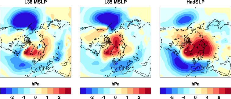
Figure 1. DJF mean L38 and L85 ensemble mean MSLP anomalies compared to observations. Note the different scales on the observed plot.
Download figure:
Standard imageIt has been argued that in 2009, positive Eurasian snow cover anomalies led to tropospheric forcing of the stratosphere, causing an SSW whose signal then descended to influence the troposphere and force a negative AO-like pattern [14]. November Eurasian snow cover area derived from NOAA satellite data has a correlation of −0.20 with the HadSLP2r DJF NAO index for 1989–2002, the negative correlation being consistent with this mechanism. However, L38 November Eurasian snow cover (measured as a fraction of the total Eurasian land area covered by snow) has a positive correlation of 0.09 with the GloSea4 DJF NAO index. (Corresponding correlations for October snow cover and DJF NAO are −0.30 for observed fields and 0.07 for L38 model runs initialized in late September.) These results suggest that snow cover does not influence the NAO through this mechanism within our forecasting system.
A second possibility is that initial positive geopotential height anomalies over the Arctic preconditioned the circulation to be negative AO type with positive Arctic geopotential height anomalies and negative anomalies at lower latitudes. This circulation pattern may be maintained through the formation of sea ice anomalies [8]. We assess this mechanism with November area mean 200 hPa height for 60–90N. The NCEP reanalysis height index has a correlation of −0.50 with the HadSLP2r DJF NAO index for 1989–2002. In the L38 GloSea4 runs, however, the height index has a correlation of only −0.04 with the GloSea4 DJF NAO index, showing that this mechanism does not explain the model signal either.
A third possibility is that low Arctic sea ice during autumn and early winter 2009 may have influenced the circulation through low-level heating anomalies [7]. Various authors (e.g. [21]) have linked low Arctic sea ice to the negative winter AO, and models suggest that European summer conditions can be remotely affected by reduced sea ice [22]. We therefore use November sea ice area (as a fraction of the total area north of 60N) as a predictor field. The HadISST sea ice index has a correlation of −0.77 with the HadSLP2r DJF NAO index for 1989–2002. The GloSea4 sea ice index has a correlation of 0.08 with the GloSea4 DJF NAO, so this mechanism is also unlikely to be operating within the model.
A fourth possible mechanism is the link between a tripole pattern in North Atlantic SST in autumn and the NAO phase in the subsequent winter [9]. This mechanism appears to have contributed to the negative NAO in winter 2009/10 [23]. However, correlating the hindcast November North Atlantic SST fields with the Glosea4 DJF NAO index does not reproduce the tripole pattern. Furthermore, the 2009/10 forecasts all have very similar November Atlantic SST fields but the SST does not resemble the tripole pattern associated with the negative NAO. This suggests that the Atlantic SST does not play a strong role in forcing the model winter NAO in the manner suggested by [9] and observations.
Since the correlations between the DJF NAO index and the predictor fields we tested are all low and insignificant in the hindcasts, the proposed mechanisms described above do not appear to explain the GloSea4 prediction of a negative NAO in winter 2009/10. This does not rule out the possibility that the mechanisms exist in reality but are not correctly simulated in the model. For example, the CMIP3 models fail to capture observed correlations between Eurasian snow cover and winter climate [24]. The mechanisms may also operate in a nonlinear way (e.g. when a threshold value is crossed) but this is difficult to test within the GloSea4 system given the relatively short hindcast period.
A remaining potential explanation for the GloSea4 model performance is the accurate prediction of an increased risk of SSWs in winter 2009/10, impacting surface climate through the mechanism described in [11]. Although the low top model cannot fully resolve SSWs, it does possess a few levels in the lower stratosphere which may permit some sensitivity of the troposphere to influences on the polar stratospheric vortex. We test this mechanism further in section 4 with the high top model configuration.
4. High top results
Previous work suggests that the stratosphere plays an important role in European winter climate, with signals from SSWs descending to the troposphere and preceding a negative Arctic Oscillation pattern [11, 25]. Both El Niño and the easterly phase of the Quasi-Biennial Oscillation (QBO) are associated with a warmer polar stratosphere in winter [26]. SSWs are more frequent during both El Niño events [27, 28] and the easterly QBO [12, 29] although the observed record shows that these links are relatively weak. The 2009/10 winter was unusual with both a clear El Niño and strong easterly QBO, both suggesting a propensity for SSWs (figure 2). In the 2009/10 winter a minor and a major SSW occurred, as discussed above.
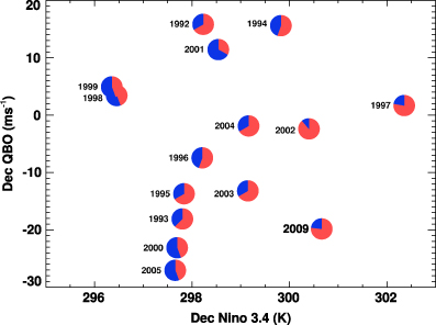
Figure 2. December Niño3.4 versus December QBO for the 2009/10 and hindcast runs. Pie charts show proportion of runs for each year with/without SSWs in red/blue.
Download figure:
Standard imageWe therefore expect the L85 model with its better resolved stratosphere to have the potential to improve on the L38 results. Unlike the L38 model, the L85 model generates realistic SSWs (defined to occur when zonal mean zonal wind at 60N, 10 hPa becomes negative during DJF). Links between SSWs and El Niño and the QBO phase may be clearer in the model runs than observations since there are multiple realizations for each year, unlike the single observed realization. The L85 runs have significantly more SSWs in winters with higher December Niño3.4 (figure 2). The fraction of ensemble members with SSWs in each winter has a correlation of 0.71 with that winter's ensemble mean December Niño3.4, significant at the 1% level. The corresponding correlations between SSW fraction and ensemble mean QBO (defined as 30 hPa zonal mean zonal wind at the equator) are −0.07, −0.28 and −0.35 for December, January and February respectively. These negative correlations are consistent with more warmings in the easterly QBO phase (all of the correlations are insignificant at the 10% level, possibly due to the limited length of the hindcast period). Both the El Niño and the easterly QBO were initialized in the L85 2009/10 forecasts, in which there are significantly more members (at the 5% level) with SSWs (77%) than the hindcast mean (58%). The latter agrees well with the observed climatological frequency [30].
The L85 runs further show the SSW events to precede a pronounced change in surface climate. There are significant differences in MSLP and 1.5 m temperature between runs with and without SSWs. In February, Arctic mean (70–90N) MSLP is 3.8 hPa higher and North European mean (15W–45E, 45–75N) temperature is 0.6 K lower for SSW minus non-SSW cases. These differences are of similar size to those shown for SSW cases minus climatology in [10]. This surface SSW signal is large enough to influence individual winters; the proportion of L85 runs for each year that contain a SSW has a correlation of 0.64 with each year's L85 ensemble mean February Arctic MSLP and a correlation of −0.70 with ensemble mean northern Europe temperature.
Figure 1 shows that the DJF mean MSLP fields from the L85 results are closer to observed MSLP than L38, with higher Arctic MSLP. Since the model MSLP fields shown are ensemble means while the observations represent a single realization, the model anomalies are much less extreme. The DJF difference between L38 and L85 is largely due to the difference in February (figure 3). This is consistent with the increased incidence of SSWs in the 2009/10 L85 runs, as SSWs occur most frequently in mid-winter and AO responses lag by between 5 and about 60 days [11]. For 2009/10, the February Arctic mean MSLP anomaly is significantly higher in the L85 ensemble mean than for L38. The observed anomaly (13.0 hPa) is just within the range of the L85 ensemble (albeit close to the largest L85 anomaly of 13.9 hPa) but well outside the L38 ensemble range (largest anomaly 7.5 hPa). Furthermore, the ensemble mean is greatly enhanced in the L85 ensemble (3.2 hPa) compared to L38 (0.0 hPa).

Figure 3. Top: L85 minus L38 ensemble mean MSLP anomalies for each month of winter 2009/10. White contours show regions where difference is significant at 5% level. Bottom: box whisker plots corresponding to the month of the plots above, with min/max and quartiles of the distribution of Arctic mean (70–90N) MSLP for the L85 (black) and L38 (red) ensembles. The blue dots show the corresponding observed values.
Download figure:
Standard imageA descending stratospheric signal is also evident in the L85 zonal mean zonal winds, shown in figure 4. The observed winds (panel (a)) have an unpredictable component due to internal variability, but nevertheless show two strong periods of easterly anomalies. The L85 zonal mean zonal wind anomalies at 60N over the winter show a structure similar to observations and that seen in other El Niño events [27]. The ensemble mean wind anomalies at 10 hPa are negative throughout the winter (panel (b)) showing the strong tendency for a negative anomaly in 2009/10. They therefore appear somewhat different to the observed winds shown in panel (a). However, the closest individual ensemble member to the observations (panel (c)) shows a striking similarity, demonstrating that ensemble members do not simply maintain a weak polar vortex initial state through the winter. Note also that the observed 10 hPa wind anomalies are within the ensemble spread throughout the winter (panel (d)).
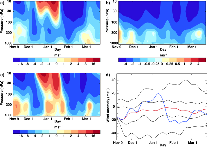
Figure 4. (a) Observed zonal mean zonal wind anomalies at 60N as a function of time for the 2009/10 winter. (b) Equivalent plot based on L85 ensemble mean wind anomalies. (c) Equivalent plot for the closest individual high top ensemble member to the observations. (d) L85 ensemble zonal mean zonal wind anomalies at 60N, 10 hPa through winter 2009/10. Red line shows ensemble median, thick black lines show ensemble 25th and 75th percentiles and thin black lines show ensemble min and max values. Blue line shows observed value. Note the smaller contour intervals in (b) compared to (a) and (c). Quantities in all panels are low pass filtered with a half power period of 20 days.
Download figure:
Standard imageFinally, we test whether the mechanism for the El Niño forcing of the SSWs in the forecasts is consistent with that described by [28]. In this mechanism, El Niño forces a deeper Aleutian Low, which in turn produces enhanced wavenumber 1 forcing of the stratosphere. Subsequent weakening of the stratospheric zonal wind and descending wave-mean flow interaction then precedes a negative AO response at the surface.
GloSea4 shows skill in forecasting El Niño [15]. In the hindcasts, December Niño3.4 has a significant correlation (at the 1% level) of −0.32 with December MSLP in the Aleutian Low region, so that El Niño events are associated with a deeper Aleutian Low. The mean December Aleutian Low MSLP for model runs that contain a SSW is significantly lower than for those that do not, so these results explain the link between higher December Niño3.4 and more SSWs shown in figure 2. Furthermore, figure 5 shows that the reduction in stratospheric westerly zonal winds is correlated with the early winter MSLP as suggested above. Ensemble members with a lower minimum zonal mean zonal wind at 60N, 10 hPa have a stronger Aleutian Low in December. These members also have a more negative AO-like response in January and February to the weaker stratospheric polar vortex, consistent with the intraseasonal response.
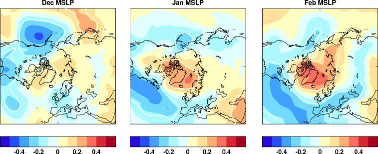
Figure 5. Correlation between SSW strength (based on minimum zonal wind at 60N, 10 hPa over the whole winter) and MSLP for L85 hindcasts. White contours show regions where correlation is significant at the 5% level.
Download figure:
Standard image5. Conclusions
We investigated the cold 2009/10 winter in high top and low top configurations of the Met Office seasonal forecast system GloSea4. Both configurations show an increased likelihood of cold, blocked conditions in the European region. The high top model predicts more intense ensemble mean circulation anomalies that more closely match the observations, particularly in late winter. The ensemble mean anomalies are much less extreme than those observed, but some ensemble members do produce anomalies of similar size to the observations. We tested several hypotheses in the hindcasts to explain the performance of the low top model but the results were all negative, suggesting that several postulated mechanisms are unlikely to explain this model result. Given the lower vertical resolution, it appears that this model responds to El Niño forcing in the same way as the high top model, but more weakly due to the limited stratospheric representation. A different model was used in [31] to investigate several possible mechanisms behind the negative NAO in winter 2009/10, but a specific cause of the observed NAO anomaly was not found.
High top runs for 2009/10 show increased number of SSWs relative to the hindcasts, consistent with the observed SSWs and the unusual precursors of an easterly phase QBO and strong El Niño. Although it is difficult to draw conclusions from a single observed event, we tested for consistency between our forecast ensemble and the observed anomaly (cf [32]).
Furthermore, the high top results are in line with previous work, both in terms of El Niño forcing of SSWs via an enhanced Aleutian Low, and also the SSW impact on surface climate, with a descending signal in zonal mean zonal wind reaching the troposphere in late winter and leading to cold, blocked conditions. Of course, factors other than El Niño also play a role in driving European winter climate, including Atlantic SST [9], volcanic eruptions [33], snow cover [14] and solar forcing [34, 35]. In particular, the anomalous snow cover and solar minimum in 2009/10 may have contributed to the observed conditions.
Each winter the atmosphere is subject to several competing influences; separating their effects remains a challenging problem, particularly given the possibility of nonlinear interactions between forcing factors [36, 37]. Unpredictable internal atmospheric variability is also likely to have contributed in 2009/10, since the most extreme seasons presumably arise through the additive combination of forced signals and weather noise. The relative sizes of each of these components in 2009/10, and in northern hemisphere winters more generally, is still unclear.
Nevertheless, given the lead time of several weeks for the SSW mechanism, the results described here are promising for enhanced forecast skill for similar exceptional events, even though average hindcast skill may be low. The high top (L85) model was incorporated into operational use in time for the 2010/11 and 2011/12 winters, during which the ensemble mean AO anomalies matched the observed values: negative in 2010/11 and positive in 2011/12.
Acknowledgments
We thank Craig MacLachlan for assistance with production of the forecast runs. This work was supported by the Joint DECC/Defra Met Office Hadley Centre Climate Programme (GA01101).
© Crown Copyright 2012, the Met Office, UK