

Abstract
The transient climate response to cumulative carbon emissions (TCRE) is a highly policy-relevant quantity in climate science. The TCRE suggests that peak warming is linearly proportional to cumulative carbon emissions and nearly independent of the emissions scenario. Here, we use simulations of the Earth System Model (ESM) from the Geophysical Fluid Dynamics Laboratory (GFDL) to show that global mean surface temperature may increase by 0.5 °C after carbon emissions are stopped at 2 °C global warming, implying an increase in the coefficient relating global warming to cumulative carbon emissions on multi-centennial timescales. The simulations also suggest a 20% lower quota on cumulative carbon emissions allowed to achieve a policy-driven limit on global warming. ESM estimates from the Coupled Model Intercomparison Project Phase 5 (CMIP5–ESMs) qualitatively agree on this result, whereas Earth System Models of Intermediate Complexity (EMICs) simulations, used in the IPCC 5th assessment report to assess the robustness of TCRE on multi-centennial timescales, suggest a post-emissions decrease in temperature. The reason for this discrepancy lies in the smaller simulated realized warming fraction in CMIP5–ESMs, including GFDL ESM2M, than in EMICs when carbon emissions increase. The temperature response to cumulative carbon emissions can be characterized by three different phases and the linear TCRE framework is only valid during the first phase when carbon emissions increase. For longer timescales, when emissions tape off, two new metrics are introduced that better characterize the time-dependent temperature response to cumulative carbon emissions: the equilibrium climate response to cumulative carbon emissions and the multi-millennial climate response to cumulative carbon emissions.
Export citation and abstract BibTeX RIS

Content from this work may be used under the terms of the Creative Commons Attribution 3.0 licence. Any further distribution of this work must maintain attribution to the author(s) and the title of the work, journal citation and DOI.
1. Introduction
In a wide set of future carbon emissions scenarios, climate model simulations (Matthews et al 2009, Gillett et al 2013) and theoretical arguments (Raupach et al 2011, Goodwin et al 2015) indicate an approximately linear relationship between cumulative carbon emissions and projected global mean temperature over the 21st century and beyond. This transient climate response to cumulative carbon emissions (TCRE) is estimated to likely (>66% likelihood) be in the range of 0.8–2.5 °C/1000 Gt carbon (IPCC 2013). TCRE is defined for peak temperature (IPCC 2013) and is nearly independent of the rate of carbon emissions (Zickfeld et al 2012, Herrington and Zickfeld 2014, Krasting et al 2014). Any global temperature target therefore implies a limited carbon emissions budget (Allen et al 2009, Matthews et al 2009). The TCRE emerges from the diminishing radiative forcing from CO2 per unit mass being compensated for by the diminishing ability of the ocean to take up heat and carbon (Matthews et al 2009, Zickfeld et al 2012, Gillett et al 2013, Goodwin et al 2015). TCRE is a useful policy framework as it establishes a simple relationship between the cause of warming, i.e. carbon emissions, and the magnitude of warming. Therefore, TCRE may play an important role in the post-Kyoto political negotiations for a new global agreement on future carbon emissions.
On multi-millennial timescales when carbon emissions tape off, the coefficient relating global warming to cumulative carbon emissions is assumed to be approximately constant or slowly decreases (Matthews et al 2009). This results out of modeling studies with Earth System Models of Intermediate Complexity (EMICs) suggesting that global mean temperature will either stabilize or decline post CO2 emissions (Plattner et al 2008, Allen et al 2009, Matthews et al 2009, Solomon et al 2009) after a decade till maximum warming occurs (Ricke et al 2014). In these EMIC models, temperature is simulated to increase after a carbon emissions stoppage on multi-centennial timescales only when equilibrium climate sensitivity (ECS) is very high (Pierrehumbert 2014), i.e. similar or larger than the top of the Intergovernmental Panel on Climate Change (IPCC) range of 2.1°–4.7° (Flato et al 2013). However, EMICs represent relevant components of the Earth System, such as cloud feedbacks or ocean physics, in a simplified manner and often at low resolution. Therefore, it is unclear if the EMIC results are robust across more complex Earth System Models (ESMs) such as those that have participated in the Coupled Model Intercomparison Project Phase 5 (CMIP5–ESMs). A recent modeling study with such a comprehensive ESM questions the usefulness of the TCRE for peak warming projections on multi-centennial to millennial timescales (Frölicher et al 2014). They find in idealized experiments that global mean temperature continues to increase on multi-centennial timescales after an instantaneous 1800 Pg carbon pulse, and after a century-long decrease in temperature. Thus, there may be a significant amount of future warming expected from past carbon emissions. These results imply that the coefficient relating global warming to cumulative carbon emissions may increase after carbon emissions tape off and that the maximum warming per unit carbon emitted may be larger than previously thought. However, it remains unclear if the ongoing warming response in the millennium following cessation of emissions is a robust feature across a wide range of different CMIP5–ESMs and under more standard carbon emissions scenarios.
This study uses the same ESM as in Frölicher et al (2014) to show that the earlier modeling results also hold under a more standard carbon emissions scenario. In addition, existing simulations of a wide range of CMIP5–ESMs and EMICs are used to show that the temperature increase after zero carbon emissions is a robust feature across CMIP5–ESMs, but rarely simulated in EMICs. We will show that the realized warming fraction—the fraction of committed warming already realized after a steady increase in radiative forcing—is key to understand the multi-centennial warming response. Finally, the study shows that the temperature response to cumulative carbon emissions can be characterized by three different timescales or phases and that the TCRE concept is only valid during the first phase, when emissions steadily increase. Two new metrics will be introduced that better characterize the long-term temperature response to cumulative carbon emissions when emissions tape off, namely the equilibrium climate response to cumulative carbon emissions (ECRE) and the multi-millennial climate response to cumulative carbon emissions (MCRE).
2. Methods
In this analysis, we use a 1000 yr simulation from the Geophysical Fluid Dynamics Laboratory ESM (GFDL ESM2M; Dunne et al 2012). We also use existing modeling data from CMIP5–ESMs (supplementary table 1, Andrews et al 2015) and from EMICs (supplementary table 2, Eby et al 2013) that participated in the CMIP5 to put the GFDL ESM2M simulations into a broader context and to test the robustness of the results. Only models that provide global mean surface temperature, an estimate of ECS and the output necessary to diagnose CO2 emissions and hence TCRE are used.
2.1. GFDL ESM2M
To visualize the time-dependent multi-centennial climate response to carbon emissions, a 1000 yr simulation with the fully coupled carbon cycle–climate model GFDL ESM2M (Dunne et al 2012) has been performed. The physical state model underlying GFDL ESM2M is an updated version of the coupled model CM2.1 (Delworth et al 2006), consisting of a 1° version of the MOM4p1 ocean model (Griffies 2009) coupled to an approximately 2° atmospheric model (AM2, Anderson et al 2004). The ocean biogeochemical model is Tracers of Ocean Phytoplankton and Allometric Zooplankton code version 2 that includes the representation of the carbon cycle. The model also includes representation of the land biogeochemistry.
The GFDL ESM2M is forced with prescribed atmospheric CO2 increasing at a rate 1% per year from preindustrial 286 to 745 ppm (year 99 of the simulation) when global annual mean surface temperature is 2 °C above preindustrial levels, after which carbon emissions stop. The diagnosed cumulative carbon emissions that are compatible with the prescribed atmospheric CO2 concentration pathway by year 99 are 1947 Gt C (gray line in figure 1(a)). Here, the carbon emissions are stopped at 2 °C global warming, as this temperature target has been widely discussed and commonly regarded as an adequate means of avoiding dangerous climate change in policy making. An extension of the standard 1% CO2 increase per year scenario has been chosen as this scenario is usually utilized to derive the TCRE (Matthews et al 2009). The CO2 emissions stoppage is a rather unrealistic setup for temperature stabilization. However, intermediate complexity model simulations suggest that this scenario gives virtually identical long-term temperature changes as when using the same amount of total cumulative carbon emissions following more realistic scenarios (Eby et al 2009). Forcing from non-CO2 greenhouse gases and other radiative forcing agents were kept at their preindustrial values throughout the simulations. Note that the GFDL ESM2M is the same model as used in the idealized carbon pulse experiment by Frölicher et al (2014). They used similar cumulative carbon emissions (1800 Gt C) and also suggest continued multi-centennial global warming after zero carbon emissions.
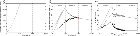
Figure 1. (a) Times series of compatible cumulative carbon emissions for a 1% rise in atmospheric CO2 until year 99, after which carbon emissions stop. (b) Time series of simulated (phase I and II) and estimated (phase III) global mean temperature changes when carbon emissions steadily increase (phase I), on multi-centennial timescales when carbon emissions cease (phase II), and on multi-millennial timescales (∼10 000 years) when ocean heat uptake is zero (phase III). (c) Times series of radiative forcing (labeled as R in units of W m−2), ocean heat uptake (labeled as N in units of W m−2) and the difference between radiative forcing and ocean heat uptake (labeled as R − N in units of W m−2). The radiative forcing has been calculated using the simplified expression R = 5.35*ln(CO2(t)/CO2(t = 0)), with CO2(t = 0) = 286 ppm. Black lines in all panels are simulated by GFDL ESM2M, whereas gray lines are estimated values (see method section for calculation details). Vertical gray dashed lines indicate phase I–III. Green, red and blue points in (b) indicate temperature change in year 99, 1000, and 10 000, respectively.
Download figure:
Standard image High-resolution imageTo estimate the GFDL ESM2M equilibrium temperature response in year 10 000 (T10 000), the ECS of the GFDL ESM2M is scaled with a factor of ln(CO2,10 000/CO2,PI)/ln(2), following the conventional form for CO2 forcing:

The ECS of 3.3 °C is estimated from a 4000 yr 1% CO2 to doubling experiment with the GFDL ESM2M model. After CO2 emissions are ceased in year 99 it takes ESM2M about an additional 900 years to be in equilibrium with the contemporaneous CO2 radiative forcing i.e. the ocean heat uptake is virtually zero (black line labeled with N in figure 1(c)). The atmospheric CO2 in year 10 000, CO2,10 000 is obtained using

with the unit conversion factor of 2.12 Gt C ppm−1, the simulated cumulative carbon emissions in year 99, emis99, of 1947 Gt C, and the preindustrial atmospheric CO2 concentration CO2,PI of 286 ppm. The GFDL ESM2M simulates an airborne fraction of anthropogenic carbon emissions, af1000, of 0.21 in year 1000. This af1000 is scaled by a factor of 0.8 under the assumption that 80% of the anthropogenic carbon emissions in year 1000 are still in the atmosphere in year 10 000 (Archer et al 2009).
2.2. CMIP5–ESMs
We use existing model data from 12 ESMs that participated in CMIP5 (supplementary table 1). The temperature time series of the first 99 years (T99) are obtained from available 1% increasing to 4xCO2 (286–1144 ppm) experiments. The temperatures in year 1000, T1000, are estimated using:
with cumulative carbon emissions in year 99, emis99, from each individual model (forth row in supplementary table 1). Here, we assume that the models are in equilibrium with the contemporaneous CO2 forcing after 1000 years, i.e. the ocean heat uptake is zero. The effective equilibrium climate sensitivities, ECS (second row in supplementary table 1), are obtained from Andrews et al (2015), who estimated the effective ECS with a linear extrapolation method using years 21–150 from CO2 instantaneously quadrupling experiments. At present, the instantaneously quadrupling experiments are usually used to estimate the ECS, but these simulations are still not long enough to accurately estimate the ECS (Frölicher et al 2014, Paynter and Frölicher 2015). This can be exemplified with the GFDL ESM2M which when run to equilibrium has an ECS of 3.3 °C, but an estimated effective ECS of 2.6 °C when using the linear extrapolation method. However, this uncertainty is small compared to the spread in ECS across the models.
The airborne fraction of carbon emissions in year 1000, af1000 = 0.25, is obtained from an average of the eight EMIC simulations (sixth row in supplementary table 2) that were run for 1000 years under a 1800 Gt C delta-pulse experiment (Eby et al 2013). 1800 Gt C is close to the 1919 ± 154 Gt C emitted in the CMIP5–ESMs by year 99 (fourth row in supplementary table 1). It has been shown that the long-term atmospheric CO2 response to a carbon pulse simulated by CMIP5–ESMs is within the uncertainty range simulated by EMICs (Joos et al 2013). To test the robustness of our results, we also use a lower (af1000,min = 0.17) and upper bound (af1000,max = 0.31) for the airborne fractions of anthropogenic CO2 emissions, which is the range simulated across the eight EMICs considered in this study (sixth row in supplementary table 2). As the CMIP5–ESMs are not run over period 99–10 000, we assume that the temperature change between years 99 and 1000 and 10 000 is linear as a function of time. The resulting change between these years is best viewed as a trend rather than the actual pathway that the model will follow.
Global mean temperature change in year 10 000 is obtained from equations (1) and (2) using emis99 and ECS of the individual models. Again, the temperature change between T1000 and T10 000 is estimated using linear interpolation between these two years.
2.3. EMICs
We also use model data from eight EMIC models to estimate the temperature response in year 99, 1000 and 10 000 using equations (1)–(3). All values are given in supplementary table 2. T99, emis99, af1000 and ECS are obtained from Eby et al (2013). Here, af1000 and T99 are both simulated by the EMIC models, but under slightly different scenarios (4xCO2 pulse experiments for af1000 and 1% CO2 increase for T99). The uncertainty in the multi-millennial temperature response for the EMICs is overall smaller than for the CMIP5–ESMs because the full range across the eight EMICs is used for the CMIP5–ESMs. Note also that the ECS estimates of the EMICs might slightly be low-biased as the ECS were obtained from relatively short 1000 yr long 2xCO2 simulation implying that the models were not yet in equilibrium, i.e. ocean heat uptake is not zero as can be seen under http://climate.uvic.ca/EMICAR5/results/4Xd/ for a similar scenario. The use of EMIC models allows us to investigate if there is a fundamental difference in the multi-centennial warming response between CMIP5–ESMs and EMICs.
3. Results
3.1. Simulated and estimated multi-millennial climate response in GFDL ESM2M
The multi-millennial climate response to carbon emissions in GFDL ESM2M can be characterized by three phases (indicated with dashed vertical lines in figure 1(b)). During phase I (years 0–99), while carbon emissions steadily increase, global mean temperature (black line in figure 1(b)) increases nearly linearly until it reaches 2 °C above preindustrial (green point in figure 1(b)). At the end of phase I, the ratio between the simulated temperature (black line in figure 1(b)) and the temperature in thermal equilibrium with the contemporaneous CO2 radiative forcing (gray line in figure 1(b)), defined as the realized warming fraction, is 0.43.
After the phase I, carbon emissions are stopped at 2 °C warming. The atmospheric CO2 is simulated to decrease from 747 ppm in year 99 to 476 pm in year 1000, indicating that 21% of the cumulative carbon emissions are still in the atmosphere in year 1000. The land carbon uptake diminishes after 200 years and the ocean is the only sink thereafter. In this post-emissions phase II (figure 1(b)), global mean temperature continues to increase on multi-centennial timescales by 0.5 °C (or by 25%) until peak temperature is reached at the end of the 1000 year simulation (red point in figure 1(b)). Although the realized warming fraction in year 99 of 0.43 implies that if CO2 were held fixed the global mean temperature would increase by a further 2.6 K, the decline in CO2 means that the actual increase by year 1000 is only a further 0.5 K.
Significant warming occurs post-emissions despite a decline in radiative forcing R that exceeds the decline in ocean heat uptake N (figure 1(c)). The difference between radiative forcing and ocean heat uptake is usually used to explain the simulated temperature response in other models (Matthews et al 2009, Solomon et al 2009). The reason for the warming in GFDL ESM2M is that decreasing ocean heat uptake warms the Earth more in the global mean than the CO2 forcing decrease is cooling. This is because the ocean heat uptake is localized in the subpolar ocean (Winton et al 2010, Frölicher et al 2014, Rose et al 2014) and perturbations at the high latitudes are restored less strongly by radiation to space than those at lower latitudes. In addition, there is no common reason to believe that the warming influence of decreasing ocean heat uptake should counteract exactly the forcing decline due to CO2 uptake (Winton et al 2013, Frölicher et al 2015). Recent analysis haven shown that ocean storage of anthropogenic carbon and heat have distinct patterns, which is not consist with the view of passive process acting on both anthropogenic carbon and heat (Frölicher et al 2015).
After 1000 years, the warming is equal to the equilibrium climate temperature with the contemporaneous CO2 levels (gray line in figure 1(b)), and both atmospheric CO2 and global mean surface temperature start to slowly decrease. In this phase III, the ocean waters pH that has decreased in phase I and II will be restored by reactions between oceanic dissolved CO2 and calcium carbonate of seafloor sediments, partly replenishing the buffer capacity of the ocean and further drawing down atmospheric CO2 (Ciais et al 2013). Assuming a decrease in the airborne fraction of anthropogenic CO2 in year 1000 by 20% to year 10 000 (see methods), the global mean temperature is estimated to be still 2.1 °C above preindustrial levels after 10 000 years (blue point in figure 1(b)) and still 0.1 °C above the temperature at the point of stopping emissions in year 99. Note that in the next several hundred thousands of years, CO2 would be restored to its preindustrial levels through reactions with silicate rocks, a very slow process of CO2 reaction with calcium silicate and other mineral of igneous rocks (Sundquist 1990). As a result, global mean temperature would slowly decrease to preindustrial levels.
Under this idealized global warming scenario, the GFDL ESM2M suggests the peak temperature change in response to cumulative carbon emissions 25% larger than the temperature change when emissions were stopped, and the multi-millennial temperature change after 10 000 years still 5% larger than the temperature change when emissions were stopped. The fact that peak temperature is larger than the temperature at the point when stopping emissions has profound implications for allowable carbon emissions to remain below a certain temperature target. This will be discussed in section 3.4.
3.2. Simulated and estimated multi-millennial climate response in CMIP5–ESMs and EMICs
Next, we will compare the GFDL ESM2M results with estimates from CMIP5–ESMs and EMICs to test the robustness of the GFDL ESM2M results and to test if CMIP5–ESMs and EMICs show a fundamentally different response. The particular carbon emissions scenario used for GFDL ESM2M has only been run over phase I by other CMIP5–ESMs and by EMICs, but the global temperature response in year 1000 and year 10 000 can be estimated using preexisting simulations (see methods).
During phase I, all models simulate a nearly linear increase in global mean temperature, consistent with earlier studies (Matthews et al 2009, Gillett et al 2013). At the end of phase I, the CMIP5–ESMs and EMICs as a class simulate similar temperature changes (2.5 ± 0.5 °C in CMIP5–ESMs; 2.5 ± 0.6 °C in EMICs; figures 2(a) and (b). Interestingly, the simulated realized warming fraction is significantly lower in CMIP5–ESMs (0.58 ± 0.06; fifth row in supplementary table 1) than in EMICs (0.70 ± 0.08; fifth row in supplementary table 2). In other words, the relative influence of the ocean in reducing the response to CO2 radiative forcing is much higher in CMIP5–ESMs than in EMICs. The simulated temperature response and the realized warming fraction is lower in GFDL ESM2M than the mean of the CMIP5–ESMs and EMICs in phase I (figures 2(a), (b), figure 1(b), supplementary table 1 and 2).
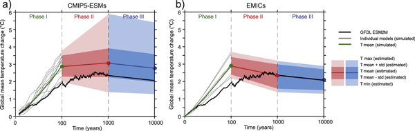
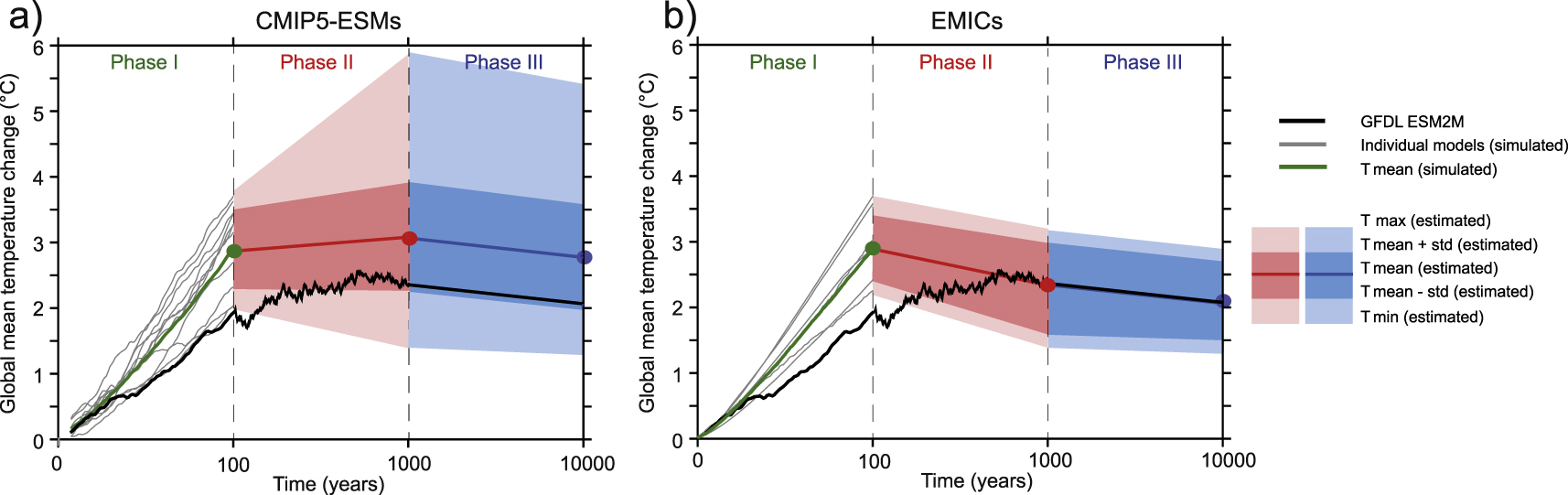
Figure 2. Global mean temperature changes simulated (phase I) and estimated (phases II and III) by (a) 12 CMIP5–ESMs and (b) 8 EMICs. Gray lines in phase I indicate the simulated temperature responses of the individual models, whereas the green, red and blue lines in phase I–III are the simulated and estimated multi-model mean temperature responses. The simulated (phase I and II) and estimated (phase III) temperature response in GFDL ESM2M is shown in black color. Note that the uncertainty ranges are calculated differently for CMIP5–ESMs and EMICs as the airborne fraction of anthropogenic CO2 emissions in year 1000 was not available for the CMIP5 models. For CMIP5–ESMs: dark red and dark blue colors in phase II and III indicate the one standard deviation uncertainty range among the models using the multi-model mean af1000 from the EMICs, and the light red and light blue colors in phase II and III indicate the maximum and minimum values when using the full af1000 range from the EMICs. For EMICS: dark red and dark blue colors in phase II and III indicate the one standard deviation uncertainty range among the models using the individual modeled af1000, and the light red and light blue colors in phase II and III indicate the maximum and minimum values when using individual modeled af1000.
Download figure:
Standard image High-resolution imageDuring phase II, the estimated temperature response between the CMIP5–ESMs (including GFDL ESM2M) and the EMICs diverge. Assuming an airborne fraction of anthropogenic CO2 of 25% at the end of phase II in year 1000 (see methods), the CMIP5–ESMs are estimated to simulate an increase in temperature of 0.2 ± 0.5 °C over the period 99–1000, whereas the EMICs as a class are estimated to simulate a decrease in temperature of −0.6 ± 0.2 °C. Note however that the uncertainties in the estimated temperature response for the CMIP5–ESMs is large, especially when additionally taking into account the uncertainties originating from the estimated airborne fraction (rows seven and eight in supplementary table 1). Here, it is assumed for all models that the climate system is in equilibrium with the contemporaneous CO2 radiative forcing in year 1000. Extending the equilibration time would not significantly change the temperature response, as the airborne fraction of atmospheric CO2 only slowly decreases after year 1000. Reducing the equilibration time, however, would lead to an additional increase in temperature after zero emissions as the airborne fraction is higher before year 1000.
During phase III (period 1000–10 000), the temperature is estimated to decrease by −0.3 °C ± 0.1 °C in the CMIP5–ESMs. The temperature in year 10 000 is only 0.1 ± 0.5 °C below the temperature in year 99 in CMIP5–ESMs when carbon emissions are ceased. The EMIC models simulate an additional temperature decrease of −0.2 ± 0.1 °C from year 1000 to 10 000.
The estimated multi-centennial decrease in temperature by the EMICs is consistent with the study by Zickfeld et al (2013) who analyzed preindustrial CO2 emissions commitment in a few future emissions scenarios with the same EMIC models. They show that even when the positive non-CO2 forcing is kept constant after zero CO2 emission, the temperature decreases on multi-centennial timescales. The few existing multi-centennial-scale modeling simulations with comprehensive ESMs show contrasting responses. The GFDL ESM2M for example, simulates ongoing warming after a CO2 emissions stoppage, not simulated by both NCAR CSM1.4-carbon (Frölicher and Joos 2010) and CanESM1 (Gillett et al 2011). The estimated multi-millennial warming responses by year 10 000 of 2.8 ± 0.8 °C per 1919 ± 154 Pg C emissions for CMIP5–ESMs and of 2.1 ± 0.6 °C per 1658 ± 90 Pg C emissions for EMICs are consistent with previous theoretical predictions of 1.6–3.8 °C per 2000 Pg C (Williams et al 2012), and qualitatively in line with single intermediate complexity model simulations that were run out for the entire 10 000 years (Eby et al 2009).
3.3. The importance of the realized warming fraction for the long-term warming response
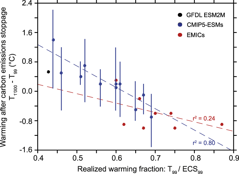
Variations in the long-term warming response between models are caused by both variations in the airborne fraction of anthropogenic carbon emissions and variations in the realized warming fraction at time when CO2 emissions cease. Figure 3 shows the relationship between the multi-centennial temperature response (T1000–T99) after zero carbon emissions and the realized warming fraction at time of zeroing carbon emissions (i.e. T99/ECS99) for all models investigated in this study. There is a nearly linear relationship between the multi-centennial temperature response and the realized warming fraction, especially in the CMIP5–ESMs. Models with low realized warming fraction show a positive multi-centennial temperature change, whereas models with high realized warming fraction show negative multi-centennial temperature change. The CMIP5–ESMs have an overall lower realized warming fraction than the EMICs and therefore show a positive temperature response post CO2 emissions. According to the CMIP5–ESMs, models with a realized warming fraction lower than 0.61 (0.47 in EMICs) are estimated to simulate ongoing warming after zero carbon emissions. One might argue that the CMIP5–ESMs results are highly uncertain as these models are not run until year 1000 and therefore the airborne fraction of the anthropogenic CO2 emission is not known. However, the EMICs, for which the airborne fractions in year 1000 are known, show a similar relationship between realized warming fraction and long-term climate change (blue dashed line for CMIP5–ESMs and red dashed line for EMICs in figure 3), although with lower confidence.
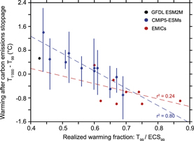
Figure 3. Relationship between the realized warming fraction, T99/ECS99, in year 99 and the global mean temperature change over the period 99–1000 (T1000–T99) after carbon emissions tape off. The black point indicates the GFDL ESM2M, blue points the CMIP5–ESMs, and red points the EMICs. The vertical blue bars for the CMIP5–ESMs indicate the uncertainty range when using T1000 with the minimum and maximum airborne fraction of anthropogenic CO2 as simulated by the EMICs (afmin and afmax; supplementary table 1). The red and blue lines show the linear regression lines using the CMIP5–ESMs and the EMICs, respectively.
Download figure:
Standard image High-resolution image3.4. Extension of the TCRE framework to multi-millennial timescales
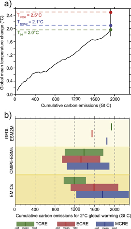
The fact that peak temperature is larger than the temperature at the point when stopping emissions in GFDL ESM2M and CMIP5–ESMs has profound implications for allowable carbon emissions to remain below a policy-driven temperature target, such as the 2 °C global warming target. As illustratively shown for GFDL ESM2M in figure 4(a), the relationship between cumulative carbon emissions and global mean temperature change shows a close to linear relationship when carbon emissions increase (phase I). This near constancy of TCRE is consistent with earlier modeling results (Mathews et al 2009, Gillet et al 2013). The simulated increase in temperature of 0.5 °C in GFDL ESM2M (from green to red point in figure 4(a)) without a change in cumulative carbon emissions during phase II and the estimated temperature decrease in phase III (from red point to blue point in figure 4(a)) cause changes in the coefficient relating global warming to cumulative carbon emissions. The increase in temperature after zero emissions in GFDL ESM2M suggest that estimates of allowable carbon emissions required to remain below the 2 °C global warming target are 20% lower (1558 Gt C instead of 1947 Gt C) than previously thought on a 1000 years timescale, and 5% lower (1854 Gt C instead of 1947 Gt C) on a 10 000 years timescale (figure 4(b)).
Figure 4. (a) Relationship between global warming and cumulative carbon emissions as simulated and estimated by GFDL ESM2M. Temperature changes in year 99, year 1000 and year 10 000 are explicitly marked with green, red and blue points and horizontal dashed lines. (b) Cumulative carbon emissions to remain below 2 °C global warming as simulated and estimated by GFDL ESM2M, CMIP5–ESMs and EMICs for TCRE, ECRE, and MCRE. The light color bands indicate the uncertainty range when using one standard deviation between the models. For the CMIP5–ESMs a mean airborne fraction of anthropogenic CO2 emissions of 0.25 as simulated by the EMICs is assumed. The uncertainty ranges would be larger when also using the full range of airborne fractions as simulated by the EMICs.
Download figure:
Standard image High-resolution image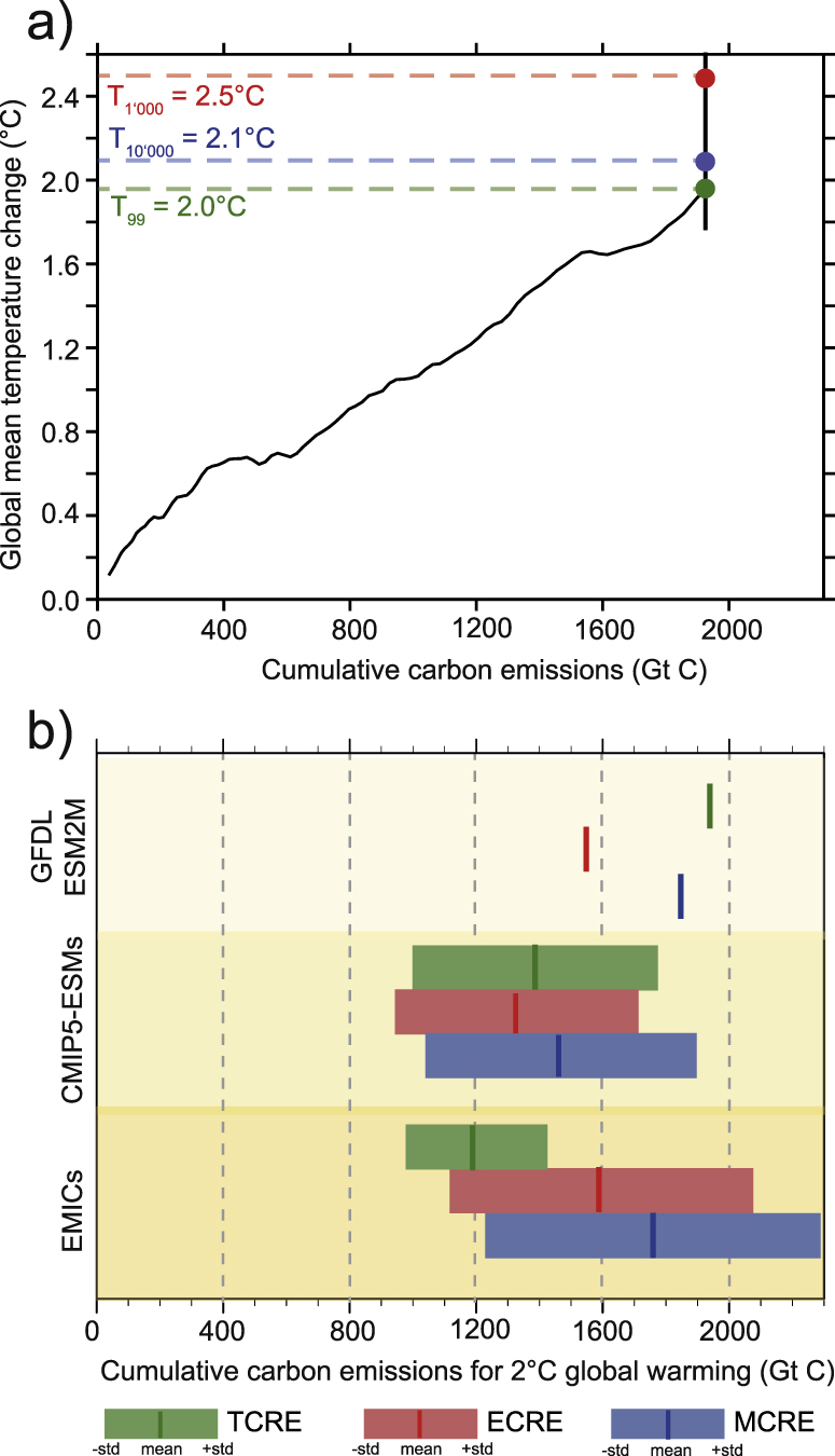
We introduce two new metrics that better characterize the time-dependent temperature response to cumulative carbon emissions, the ECRE and the MCRE. The ECRE is calculated by using the temperature change at the time when ocean heat uptake is zero, i.e. in year 1000 when the system is in equilibrium with its contemporaneous CO2 forcing, and then by dividing this by the cumulative CO2 emissions up to this time. Usually, ECS is defined as the change in global mean temperature that results when the climate system attains a new equilibrium with the radiative forcing change resulting from a doubling of atmospheric CO2. In our particular simulation, atmospheric CO2 will further decrease. Therefore, we also introduce the MCRE, which takes into account the decrease in atmospheric CO2. The MCRE is calculated identically to the ECRE, but defined on multi-millennial timescales (at year 10 000) when the exchange of carbon between the atmosphere and global ocean ceases (i.e. the ocean and land biosphere are in equilibrium with the contemporaneous atmospheric CO2), and only weathering with silicate rocks can restore atmospheric CO2 levels to preindustrial.
Applying the TCRE, ECRE and MCRE to a 2 °C global warming target in CMIP5–ESMs, TCRE is 1388 ± 388 Gt C, ECRE is 1328 ± 389 Gt C and MCRE is 1465 ± 427 Gt C (figure 4(b)). Thus, MCRE is 6% larger than TCRE, but ECRE is 4% smaller than TCRE in CMIP5–ESMs. This implies that less carbon emissions are required to hit the 2 °C target when using ECRE than when using TCRE. This is not the case for EMICs, for which peak temperature response is attained when carbon emissions are ceased and therefore ECRE (1590 ± 482 Gt C) and MCRE (1760 ± 536 Gt C) are generally larger than TCRE (1189 ± 224 Gt C; figure 4(b)).
4. Discussion and conclusions
The multi-millennial temperature response to cumulative carbon emissions have been simulated and estimated for a range of ESMs of different complexities. The GFDL ESM2M model illustratively shows that stopping carbon emissions at 2 °C global warming would mean a peak warming of 2.5 °C on multi-centennial timescales, and an irreversible warming of 2.1 °C on multi-millennial time-scales. CMIP5–ESMs as a class qualitatively confirm this result, but EMICs, which are usually used for long-term climate response simulations, show a decrease in global mean temperature after zero carbon emissions. The reason for the differences in the global warming response between CMIP5–ESMs and EMICs lies in the different simulated realized warming fractions in the two types of models, with the CMIP5–ESMs generally have a lower realized warming fraction than the EMICs when atmospheric CO2 increases. Therefore, models with generally lower realized warming fractions should be used to complete the assessment of multi-century warming response to cumulative carbon emissions and to determine the emissions budget needed to remain below a particular warming target. This will likely require the use of comprehensive ESMs rather than EMICs since the former have lower realized warming fraction. The results of the CMIP5–ESMs also indicate that the full climate damages expected to occur in response to CO2 emissions will be felt by future generations not responsible for those emissions.
Clearly, the robustness of the results needs to be tested by explicitly running the CMIP5–ESMs over multi-centennial timescales. Also, an accurate estimate of ECS is essential to estimate the realized warming fraction and the multi-centennial warming response. The effective ECS used in this study for the CMIP5–ESMs are likely biased low as they are obtained from relatively short 150 year instantaneously quadrupling experiments. Therefore, the warming responses in CMIP5–ESMs during phase II are likely low estimates. In addition, we only consider cumulative carbon emissions up to approximately 2000 Gt C. It has been shown, however that the temperature may increase on multi-centennial timescales for cumulative emissions larger than 2000 Gt C in pulse simulations with models that otherwise simulate a decrease in temperature (Matthews et al 2009, Herrington and Zickfeld 2014). Nevertheless, we show here that even with cumulative carbon emissions of about 2000 Gt C, the CMIP5–ESMs as a class show an increase in global mean temperature on multi-centennial timescales after stopping emissions.
In this study, we only consider physical and carbon–climate feedbacks that are incorporated in comprehensive ESMs. Many potentially strong positive feedbacks and abrupt changes or tipping point that arise from nonlinearity's within the climate system associated for example with the release of methane hydrates or large amounts of carbon from permafrost are not included in ESMs and are not considered in this study (see Collins et al 2013 for an extended discussion about potentially abrupt or irreversible changes). Such tipping points and feedbacks may drastically increase the global warming response to cumulative carbon emissions and may decrease the permissible carbon emissions. However, the timing of these abrupt changes and feedbacks, if any, are difficult to predict.
These new results have important implications for carbon emissions budgets. In fact, allowable carbon emissions for any future (peak) global warming limit, such as the 2 °C target, may be significantly lower than previously thought and stated in IPCC AR5. According to the GFDL ESM2M, cumulative carbon emissions to remain below 2 °C are 20% lower when using ECRE and 5% lower when using MCRE instead of TCRE. When negotiating global carbon budgets for multi-centennial warming targets, this needs to be taken into account. However, large uncertainties in the TCRE, ECRE and MCRE remain and introduce large uncertainty in the maximum cumulative carbon emissions allowed to restrict CO2-induced warming to a policy driven target. Therefore, additional efforts should be devoted to identify the sources of uncertainties in all three metrics and to ultimately reduce them. This will most likely include the reduction in the spread of ECS estimates across the models.
Acknowledgments
We thank M Eby for providing the airborne fraction values for the EMICs, T Andrews for providing the equilibrium climate sensitivity estimates of the CMIP5–ESMs, and J Roegelj for providing CMIP5–ESM data. We also thank R Knutti, N Gruber, M Winton and M Münnich for useful discussions and comments on the manuscript. T L Frölicher acknowledges financial support from the SNSF (Ambizione grant PZ00P2_142573).