


ABSTRACT
We present cosmological parameter constraints based on the final nine-year Wilkinson Microwave Anisotropy Probe (WMAP) data, in conjunction with a number of additional cosmological data sets. The WMAP data alone, and in combination, continue to be remarkably well fit by a six-parameter ΛCDM model. When WMAP data are combined with measurements of the high-l cosmic microwave background anisotropy, the baryon acoustic oscillation scale, and the Hubble constant, the matter and energy densities, Ωbh2, Ωch2, and ΩΛ, are each determined to a precision of ∼1.5%. The amplitude of the primordial spectrum is measured to within 3%, and there is now evidence for a tilt in the primordial spectrum at the 5σ level, confirming the first detection of tilt based on the five-year WMAP data. At the end of the WMAP mission, the nine-year data decrease the allowable volume of the six-dimensional ΛCDM parameter space by a factor of 68,000 relative to pre-WMAP measurements. We investigate a number of data combinations and show that their ΛCDM parameter fits are consistent. New limits on deviations from the six-parameter model are presented, for example: the fractional contribution of tensor modes is limited to r < 0.13 (95% CL); the spatial curvature parameter is limited to  ; the summed mass of neutrinos is limited to ∑mν < 0.44 eV (95% CL); and the number of relativistic species is found to lie within Neff = 3.84 ± 0.40, when the full data are analyzed. The joint constraint on Neff and the primordial helium abundance, YHe, agrees with the prediction of standard big bang nucleosynthesis. We compare recent Planck measurements of the Sunyaev–Zel'dovich effect with our seven-year measurements, and show their mutual agreement. Our analysis of the polarization pattern around temperature extrema is updated. This confirms a fundamental prediction of the standard cosmological model and provides a striking illustration of acoustic oscillations and adiabatic initial conditions in the early universe.
Export citation and abstract BibTeX RIS
1. INTRODUCTION
Measurements of temperature and polarization anisotropy in the cosmic microwave background (CMB) have played a major role in establishing and sharpening the standard "ΛCDM" model of cosmology: a six-parameter model based on a flat universe, dominated by a cosmological constant, Λ, and cold dark matter (CDM), with initial Gaussian, adiabatic fluctuations seeded by inflation. This model continues to describe all existing CMB data, including the Wilkinson Microwave Anisotropy Probe (WMAP) nine-year data presented in this paper and its companion paper (Bennett et al. 2013), the small-scale temperature data (Das et al. 2011b; Keisler et al. 2011; Reichardt et al. 2012; Story et al. 2012), and the small-scale polarization data (Brown et al. 2009; Chiang et al. 2010; QUIET Collaboration 2011, 2012).
Despite its notable success at describing all current cosmological data sets, the standard model raises many questions: What is the nature of dark matter and dark energy? What is the physics of inflation? Further, there are open questions about more immediate physical parameters: Are there relativistic species present at the decoupling epoch beyond the known photons and neutrinos? What is the mass of the neutrinos? Is the primordial helium abundance consistent with big bang nucleosynthesis (BBN)? Are the initial fluctuations adiabatic? Tightening the limits on these parameters is as important as measuring the standard ones. Over the past decade WMAP has provided a wealth of cosmological information which can be used to address the above questions. In this paper, we present the final, nine-year constraints on cosmological parameters from WMAP.
The paper is organized as follows. In Section 2, we briefly describe the nine-year WMAP likelihood code, the external data sets used to complement WMAP data, and we update our parameter estimation methodology. Section 3 presents nine-year constraints on the minimal six-parameter ΛCDM model. Section 4 presents constraints on parameters beyond the standard model, such as the tensor-to-scalar ratio, the running spectral index, the amplitude of isocurvature modes, the number of relativistic species, the mass of neutrinos, spatial curvature, the equation of state parameters of dark energy, and cosmological birefringence. In Section 5, we discuss constraints on the amplitude of matter fluctuations, σ8, derived from other astrophysical data sets. Section 6 compares WMAP's seven-year measurements of the Sunyaev–Zel'dovich (SZ) effect with recent measurements by Planck. In Section 7, we update our analysis of polarization patterns around temperature extrema, and we conclude in Section 8.
2. METHODOLOGY UPDATE
Before discussing cosmological parameter fits in the remaining part of the paper, we summarize changes in our parameter estimation methodology and our choice of input data sets. In Section 2.1 we review changes to the WMAP likelihood code. In Section 2.2 we discuss our choice of external data sets used to complement WMAP data in various tests. Most of these data sets are new since the seven-year data release. We conclude with some updates on our implementation of Markov Chains.
2.1. WMAP Likelihood Code
For the most part, the structure of the likelihood code remains as it was in the seven-year WMAP data release. However, instead of using the Monte Carlo Apodised Spherical Transform EstimatoR (MASTER) estimate (Hivon et al. 2002) for the l > 32 TT spectrum, we now use an optimally estimated power spectrum and errors based on the quadratic estimator from Tegmark et al. (1997), as discussed in detail in Bennett et al. (2013). This l > 32 TT spectrum is based on the template-cleaned V- and W-band data, and the KQ85y9 sky mask (see Bennett et al. (2013) for an update on the analysis masks). The likelihood function for l > 32 continues to use the Gaussian plus log-normal approximation described in Bond et al. (1998) and Verde et al. (2003).
The l ⩽ 32 TT spectrum uses the Blackwell–Rao estimator, as before. This is based on Gibbs samples obtained from a nine-year one-region bias-corrected Internal Linear Combination map described in (Bennett et al. 2013) and sampled outside the KQ85y9 sky mask. The map and mask were degraded to HEALPix r5,18 and 2 μK of random noise was added to each pixel in the map.
The form of the polarization likelihood is unchanged. The l > 23 TE spectrum is based on a MASTER estimate and uses the template-cleaned Q-, V-, and W-band maps, evaluated outside the KQ85y9 temperature and polarization masks. The l ⩽ 23 TE, EE, and BB likelihood retains the pixel-space form described in Appendix D of Page et al. (2007). The inputs are template-cleaned Ka-, Q-, and V-band maps and the HEALPix r3 polarization mask used previously.
As before, the likelihood code accounts for several important effects: mode coupling due to sky masking and non-uniform pixel weighting (due to non-uniform noise), beam window function uncertainty, which is correlated across the entire spectrum, and residual point source subtraction uncertainty, which is also highly correlated. The treatment of these effects is described in Verde et al. (2003), Nolta et al. (2009), and Dunkley et al. (2009).
2.2. External Data Sets
2.2.1. Small-scale CMB Measurements
Since the time when the seven-year WMAP analyses were published, there have been new measurements of small-scale CMB fluctuations by the Atacama Cosmology Telescope (ACT; Fowler et al. 2010; Das et al. 2011b) and the South Pole Telescope (SPT; Keisler et al. 2011; Reichardt et al. 2012). They have reported the angular power spectrum at 148 and 217 GHz for ACT, and at 95, 150, and 220 GHz for SPT, to 1' resolution, over ∼1000 deg2 of sky. At least seven acoustic peaks are observed in the angular power spectrum, and the results are in remarkable agreement with the model predicted by the WMAP seven-year data (Keisler et al. 2011).
Figure 1 shows data from ACT and SPT at 150 GHz, which constitutes the extended CMB data set used extensively in this paper (subsequently denoted "eCMB"). We incorporate the SPT data from Keisler et al. (2011), using 47 band-powers in the range 600 < l < 3000. The likelihood is assumed to be Gaussian, and we use the published band-power window functions and covariance matrix, the latter of which accounts for noise, beam, and calibration uncertainty. Following the treatment of the ACT and SPT teams, we account for residual extragalactic foregrounds by marginalizing over three parameters: the Poisson and clustered point source amplitudes, and the SZ amplitude (Keisler et al. 2011). For ACT we use the 148 GHz power spectrum from Das et al. (2011b) in the multipole range 500 < l < 10000, marginalizing over the same clustered point source and SZ amplitudes as in the SPT likelihood, but over a separate Poisson source amplitude. See Sections 2.3 and 3.2 for more details.

Figure 1. Compilation of the CMB data used in the nine-year WMAP analysis. The WMAP data are shown in black, the extended CMB data set—denoted "eCMB" throughout—includes SPT data in blue (Keisler et al. 2011) and ACT data in orange, (Das et al. 2011b). We also incorporate constraints from CMB lensing published by the SPT and ACT groups (not shown). The ΛCDM model fit to the WMAP data alone (shown in gray) successfully predicts the higher-resolution data.
Download figure:
Standard image High-resolution imageIn addition to the temperature spectra, both ACT and SPT have estimated the deflection spectra due to gravitational lensing (Das et al. 2011a; van Engelen et al. 2012). These measurements are consistent with predictions of the ΛCDM model fit to WMAP. When we incorporate SPT and ACT data in the nine-year analysis, we also include the lensing likelihoods provided by each group19 to further constrain parameter fits.
New observations of the CMB polarization power spectra have also been released by the QUIET experiment (QUIET Collaboration 2011, 2012); their TE and EE polarization spectra are in excellent agreement with predictions based primarily on WMAP temperature fluctuation measurements. These data are the most recent in a series of polarization measurements at l ≳ 50. However, high-l polarization observations do not (yet) substantially enhance the power of the full data to constrain parameters, so we do not include them in the nine-year analysis.
2.2.2. Baryon Acoustic Oscillations
The acoustic peak in the galaxy correlation function has now been detected over a range of redshifts from z = 0.1 to z = 0.7. This linear feature in the galaxy data provides a standard ruler with which to measure the distance ratio, DV/rs, the distance to objects at redshift z in units of the sound horizon at recombination, independent of the local Hubble constant. In particular, the observed angular and radial baryon acoustic oscillation (BAO) scales at redshift z provide a geometric estimate of the effective distance,

where DA(z) is the angular diameter distance and H(z) is the Hubble parameter. The measured ratio DV/rs, where rs is the co-moving sound horizon scale at the end of the drag era, can be compared to theoretical predictions.
Since the release of the seven-year WMAP data, the acoustic scale has been more precisely measured by the Sloan Digital Sky Survey (SDSS) and SDSS-III Baryon Oscillation Spectroscopic Survey (BOSS) galaxy surveys, and by the WiggleZ and 6dFGS surveys. Previously, over half a million galaxies and luminous red galaxies from the SDSS-DR7 catalog had been combined with galaxies from 2dFGRS by Percival et al. (2010) to measure the acoustic scale at z = 0.2 and z = 0.35. (These data were used in the WMAP seven-year analysis; see also Kazin et al. 2010). Using the reconstruction method of Eisenstein et al. (2007), an improved estimate of the acoustic scale in the SDSS-DR7 data was made by Padmanabhan et al. (2012), giving DV(0.35)/rs = 8.88 ± 0.17, and reducing the uncertainty from 3.5% to 1.9%. More recently the SDSS-DR9 data from the BOSS survey has been used to estimate the BAO scale of the CMASS sample. They report DV(0.57)/rs = 13.67 ± 0.22 for galaxies in the range 0.43 < z < 0.7 (at an effective redshift z = 0.57; Anderson et al. 2012). This result is used to constrain cosmological models in Sánchez et al. (2012).
The acoustic scale has also been measured at higher redshift using the WiggleZ galaxy survey. Blake et al. (2012) report distances in three correlated redshift bins between 0.44 and 0.73. At lower redshift, z = 0.1, a detection of the BAO scale has been made using the 6dFGS survey (Beutler et al. 2011). These measurements are summarized in Table 1, and plotted as a function of redshift in Figure 19 of Anderson et al. (2012), together with the best-fit ΛCDM model prediction from the WMAP seven-year analysis (Komatsu et al. 2011). The BAO data are consistent with the CMB-based prediction over the measured redshift range.
Table 1. BAO Data Used in the Nine-year Analysis
| Redshift | Data Set | rs/DV(z) | Ref. |
|---|---|---|---|
| 0.1 | 6dFGS | 0.336 ± 0.015 | Beutler et al. (2011) |
| 0.35 | SDSS-DR7-rec | 0.113 ± 0.002a | Padmanabhan et al. (2012) |
| 0.57 | SDSS-DR9-rec | 0.073 ± 0.001a | Anderson et al. (2012) |
| 0.44 | WiggleZ | 0.0916 ± 0.0071 | Blake et al. (2012) |
| 0.60 | WiggleZ | 0.0726 ± 0.0034 | Blake et al. (2012) |
| 0.73 | WiggleZ | 0.0592 ± 0.0032 | Blake et al. (2012) |
Note. aFor uniformity, the SDSS values given here have been inverted from the published values: DV(0.35)/rs = 8.88 ± 0.17, and DV(0.57)/rs = 13.67 ± 0.22.
Download table as: ASCIITypeset image
For the nine-year analysis, we incorporate these data into a likelihood of the form

where

and

The model distances are derived from the ΛCDM parameters using the same scheme we used in the WMAP seven-year analysis (Komatsu et al. 2011).
2.2.3. Hubble Parameter
It is instructive to combine WMAP measurements with measurements of the current expansion rate of the universe. Recent advances in the determination of the Hubble constant have been made since the two teams using Hubble Space Telescope (HST)/WFPC2 observations reported their results (Freedman et al. 2001; Sandage et al. 2006). Re-anchoring the HST Key Project distance ladder technique, Freedman et al. (2012) report a significantly improved result of H0 = 74.3 ± 1.5 (statistical) ±2.1 (systematic) km s−1 Mpc−1. The overall 3.5% uncertainty must be taken with some caution, however, since the uncertainties in all rungs are not fully propagated.
In a parallel approach, Riess et al. (2009) redesigned the distance ladder and its observations to control the systematic errors that dominated the measurements. These steps include: the elimination of zero-point uncertainties by use of the same photometric system across the ladder, observations of Cepheids in the near-infrared to reduce extinction and sensitivity to differences in chemical abundance (the so-called "metallicity effect"), the use of geometric distance measurements to provide a reliable absolute calibration, and the replacement of old Type Ia supernovae observations with recent ones that use the same photometric systems that define the Hubble flow. This approach has led to a measurement of H0 = 73.8 ± 2.4 km s−1 Mpc−1 (Riess et al. 2011) with a fully propagated uncertainty of 3.3%. Since this uncertainty is smaller, we adopt it in our analysis.
2.2.4. Type Ia Supernovae
The first direct evidence for acceleration in the expansion of the universe came from measurements of luminosity distance as a function of redshift using Type Ia supernovae as standard candles (Riess et al. 1998; Schmidt et al. 1998; Perlmutter et al. 1999). Numerous follow-up observations have been made, extending these early measurements to higher redshift. After the seven-year WMAP analysis was published, the Supernova Legacy Survey analyzed their three-year sample ("SNLS3") of high redshift supernovae (Guy et al. 2010; Conley et al. 2011; Sullivan et al. 2011). They measured 242 Type Ia supernovae in the redshift range 0.08 < z < 1.06, three times more than their first-year sample (Astier et al. 2006). The SNLS team combined the 242 SNLS3 supernovae with 123 SNe at low redshift (Hamuy et al. 1996; Riess et al. 1999; Jha et al. 2006; Hicken et al. 2009; Contreras et al. 2010), 93 SNe from the SDSS supernovae search (Holtzman et al. 2008), and 14 SNe at z > 1 from HST measurements by Riess et al. (2007) to form a sample of 472 SNe. All of these supernovae were re-analyzed using both the SALT2 and SiFTO light curve fitters, which give an estimate of the SN peak rest-frame B-band apparent magnitude at the epoch of maximum light in that filter.
Sullivan et al. (2011) carry out a cosmological analysis of this combined data, accounting for systematic uncertainties including common photometric zero-point errors and selection effects. They adopt a likelihood of the form

where mB is the peak-light apparent magnitude in B-band for each supernova,  is the corresponding magnitude predicted by the model, and C is the covariance matrix of the data. Their analysis assigns three terms to the covariance matrix, C = Dstat + Cstat + Csys, where Dstat contains the independent (diagonal) statistical errors for each supernova, Cstat includes the statistical errors that are correlated by the light-curve fitting, and Csys has eight terms to track systematic uncertainties, including calibration errors, Milky Way extinction, and redshift evolution. The theoretical magnitude for each supernova is modeled as

where  is the empirical intercept of the
  relation. The parameters α and β quantify the stretch–luminosity and color–luminosity relationships, and the statistical error, Cstat, is coupled to both parameters. Assuming a constant w model, Sullivan et al. (2011) measure α = 1.37 ± 0.09, and β = 3.2 ± 0.1. Including the term Csys has a significant effect: it increases the error on the dark energy equation of state, σw from 0.05 to 0.08 in a flat universe.
The 472 Type Ia supernovae used in the SNLS3 analysis are consistent with the ΛCDM model predicted by WMAP (Sullivan et al. 2011), thus we can justify including these data in the present analysis. However, the extensive study presented by the SNLS team shows that a significant level of systematic error still exists in current supernova observations. Hence we restrict our use of supernova data in this paper to the subset of models that examine the dark energy equation of state. When SNe data are included, we marginalize over the three parameters α, β, and M. α and β are sampled in the Markov Chain Monte Carlo (MCMC) chains, while M is marginalized analytically (Lewis & Bridle 2002).
2.3. Markov Chain Methodology
As with previous WMAP analyses, we use MCMC methods to evaluate the likelihood of cosmological parameters. Aside from incorporating new likelihood codes for the external data sets described above, the main methodological update for the nine-year analysis centers on how we marginalize over SZ and point source amplitudes when analyzing multiple CMB data sets (i.e., "WMAP+eCMB"). We have also incorporated updates to the Code for Anisotropies in the Microwave Background (CAMB; Lewis et al. 2000), as described in Section 2.3.1.
SZ amplitude. When combining data from multiple CMB experiments (WMAP, ACT, SPT) we sample and marginalize over a single SZ amplitude, ASZ, that parameterizes the SZ contribution to all three data sets. To do so, we adopt a common SZ power spectrum template, and scale it to each experiment as follows. Battaglia et al. (2012b) compute a nominal SZ power spectrum at 150 GHz for the SPT experiment (their Figure 5, left panel, blue curve). We adopt this curve as a spectral template and scale it by a factor of 1.05 and 3.6 to describe the relative SZ contribution at 148 GHz (for ACT) and 61 GHz (for WMAP), respectively. The nuisance parameter ASZ then multiplies all three SZ spectra simultaneously.
The above frequency scaling assumes a thermal SZ spectrum. For WMAP we assume an effective frequency of 61 GHz, even though the WMAP power spectrum includes 94 GHz data. We ignore this error because WMAP data provide negligible constraints on the SZ amplitude when analyzed on their own. In the SPT and ACT frequency range, the thermal SZ spectrum is very similar to the kinetic SZ spectrum, so our procedure effectively accounts for that contribution as well.
Clustered point sources. We adopt a common parameterization for the clustered point source contribution to both the ACT and SPT data, namely l(l + 1)Cl/2π = Acps l0.8 (Addison et al. 2012). Both the ACT and SPT teams use this form in their separate analyses at high l. (At low l, the SPT group adopts a constant spectrum, but this makes a negligible difference to our analysis.) By using a common amplitude for both experiments, we introduce one additional nuisance parameter.
Poisson point sources. For unclustered residual point sources we adopt the standard power spectrum Cl = const. Since the ACT and SPT groups use different algorithms for identifying and removing bright point sources, we allow the templates describing the residual power to have different amplitudes for the two experiments. This adds two additional nuisance parameters to our chains.
2.3.1. CAMB
Model power spectra are computed using the CAMB (Lewis et al. 2000), which is based on the earlier code CMBFAST (Seljak & Zaldarriaga 1996). We use the 2012 January version of CAMB throughout the nine-year analysis except when evaluating the (w0, wa) model, where we adopted the 2012 October version. We adopt the default version of recfast that is included with CAMB instead of other available options. As in the seven-year analysis, we fix the reionization width to be Δz = 0.5. Since the WMAP likelihood code only incorporates low l BB data (with low sensitivity), we set the accurate_BB flag to FALSE and run the code with  . We set the high_accuracy_default flag to TRUE. When calling the ACT and SPT likelihoods, we set k_eta_max_scalar = 15000 and l_max_scalar = 6000. The ACT likelihood extends to l = 10000, but foregrounds dominate beyond l ≈ 3000 (Dunkley et al. 2011), so this choice of lmax is conservative. Except when exploring neutrino models, we adopt zero massive neutrinos and the nominal effective number of massless neutrino species. The CMB temperature is set to 2.72548 K (Fixsen 2009).
3. THE SIX-PARAMETER ΛCDM MODEL
In this section we discuss the determination of the standard ΛCDM parameters, first using only the nine-year WMAP data, then, in turn, combined with the additional data sets discussed in Section 2.2. Our analysis employs the same MCMC formalism used in previous analyses (Spergel et al. 2003; Verde et al. 2003; Spergel et al. 2007; Dunkley et al. 2009; Komatsu et al. 2009; Larson et al. 2011; Komatsu et al. 2011). This formalism naturally produces parameter likelihoods that are marginalized over all other fit parameters in the model. Throughout this paper, we quote best-fit values as the mean of the marginalized likelihood, unless otherwise stated (e.g., mode or upper limits). Lower and upper error limits correspond to the 16% and 84% points in the marginalized cumulative distribution, unless otherwise stated.
The six parameters of the basic ΛCDM model are: the physical baryon density, Ωbh2, the physical CDM density, Ωch2, the dark energy density, in units of the critical density,  , the amplitude of primordial scalar curvature perturbations,
  at k = 0.002 Mpc−1, the power-law spectral index of primordial density (scalar) perturbations, ns, and the reionization optical depth, τ. In this model, the Hubble constant, H0 = 100 h km s−1 Mpc−1, is implicitly determined by the flatness constraint, Ωb + Ωc + ΩΛ = 1. A handful of parameters in this model take assumed values that we further test in Section 4; other parameters may be derived from the fit, as in Table 2. Throughout this paper we assume the initial fluctuations are adiabatic and Gaussian distributed (see Bennett et al. (2013) for limits on non-Gaussian fluctuations from the nine-year WMAP data) except in Section 4.2 where we allow the initial fluctuations to include an isocurvature component.
Table 2. Maximum Likelihood ΛCDM Parametersa
| Parameter | Symbol | WMAP Data | Combined Datab |
|---|---|---|---|
| Fit ΛCDM Parameters | |||
| Physical baryon density | Ωbh2 | 0.02256 | 0.02240 |
| Physical cold dark matter density | Ωch2 | 0.1142 | 0.1146 |
| Dark energy density (w = −1) |  |
0.7185 | 0.7181 |
| Curvature perturbations, k0 = 0.002 Mpc−1 |  |
2.40 | 2.43 |
| Scalar spectral index | ns | 0.9710 | 0.9646 |
| Reionization optical depth | τ | 0.0851 | 0.0800 |
| Derived Parameters | |||
| Age of the universe (Gyr) | t0 | 13.76 | 13.75 |
| Hubble parameter, H0 = 100 h km s−1 Mpc−1 | H0 | 69.7 | 69.7 |
| Density fluctuations @ 8 h−1 Mpc | σ8 | 0.820 | 0.817 |
| Baryon density/critical density | Ωb | 0.0464 | 0.0461 |
| Cold dark matter density/critical density | Ωc | 0.235 | 0.236 |
| Redshift of matter-radiation equality | zeq | 3273 | 3280 |
| Redshift of reionization | zreion | 10.36 | 9.97 |
Notes. aThe maximum-likelihood ΛCDM parameters for use in simulations. Mean parameter values, with marginalized uncertainties, are reported in Table 4. b"Combined data" refers to WMAP+eCMB+BAO+H0.
Download table as: ASCIITypeset image
To assess WMAP data consistency, we begin with a comparison of the nine-year and seven-year results (Komatsu et al. 2011); we then study the ΛCDM constraints imposed by the nine-year WMAP data, in conjunction with the most recent external data sets available.
3.1. Comparison with Seven-year Fits
Table 3 gives the best-fit ΛCDM parameters (mean and standard deviation, marginalized over all other parameters) for selected nine-year and seven-year data combinations. In the case where only WMAP data are used, we evaluate parameters using both the C−1-weighted spectrum and the MASTER-based one. For the case where we include BAO and H0 priors, we use only the C−1-weighted spectrum for the nine-year WMAP data, and we update the priors, as per Section 2.2. The seven-year results are taken from Table 1 of Komatsu et al. (2011).
Table 3. WMAP Seven-year to Nine-year Comparison of the Six-parameter ΛCDM Modela
| Parameter | WMAP-onlyb | WMAP+BAO+H0b | |||
|---|---|---|---|---|---|
| Nine-year | Nine-year (MASTER)c | Seven-year | Nine-year | Seven-year | |
| Fit parameters | |||||
| Ωbh2 | 0.02264 ± 0.00050 | 0.02243 ± 0.00055 |  |
0.02266 ± 0.00043 | 0.02255 ± 0.00054 |
| Ωch2 | 0.1138 ± 0.0045 | 0.1147 ± 0.0051 | 0.1120 ± 0.0056 | 0.1157 ± 0.0023 | 0.1126 ± 0.0036 |
 |
0.721 ± 0.025 | 0.716 ± 0.028 |  |
0.712 ± 0.010 | 0.725 ± 0.016 |
 |
2.41 ± 0.10 | 2.47 ± 0.11 | 2.43 ± 0.11 |  |
2.430 ± 0.091 |
| ns | 0.972 ± 0.013 | 0.962 ± 0.014 | 0.967 ± 0.014 | 0.971 ± 0.010 | 0.968 ± 0.012 |
| τ | 0.089 ± 0.014 | 0.087 ± 0.014 | 0.088 ± 0.015 | 0.088 ± 0.013 | 0.088 ± 0.014 |
| Derived parameters | |||||
| t0 (Gyr) | 13.74 ± 0.11 | 13.75 ± 0.12 | 13.77 ± 0.13 | 13.750 ± 0.085 | 13.76 ± 0.11 |
| H0 (km s−1 Mpc−1) | 70.0 ± 2.2 | 69.7 ± 2.4 | 70.4 ± 2.5 | 69.33 ± 0.88 | 70.2 ± 1.4 |
| σ8 | 0.821 ± 0.023 | 0.818 ± 0.026 |  |
0.830 ± 0.018 | 0.816 ± 0.024 |
| Ωb | 0.0463 ± 0.0024 | 0.0462 ± 0.0026 | 0.0455 ± 0.0028 | 0.0472 ± 0.0010 | 0.0458 ± 0.0016 |
| Ωc | 0.233 ± 0.023 | 0.237 ± 0.026 | 0.228 ± 0.027 |  |
0.229 ± 0.015 |
| zreion | 10.6 ± 1.1 | 10.5 ± 1.1 | 10.6 ± 1.2 | 10.5 ± 1.1 | 10.6 ± 1.2 |
Notes. aComparison of six-parameter ΛCDM fits with seven-year and nine-year WMAP data, with and without BAO and H0 priors. bThe first three data columns give results from fitting to WMAP data only. The last two columns give results when BAO and H0 priors are added. As discussed in Section 2.2, these priors have been updated for the nine-year analysis. The seven-year results are taken directly from Table 1 of Komatsu et al. (2011). cUnless otherwise noted, the nine-year WMAP likelihood uses the C−1-weighted power spectrum whereas the seven-year likelihood used the MASTER-based spectrum. The column labeled "Nine-year (MASTER)" is a special run for comparing to the seven-year results.
Download table as: ASCIITypeset image
3.1.1. WMAP Data Alone
We first compare seven-year and nine-year results based on the MASTER spectra. Table 3 shows that the nine-year ΛCDM parameters are all within 0.5σ of each other, with Ωch2 having the largest difference. We note that the combination  is approximately constant between the two models, reflecting the fact that this combination is well constrained by primary CMB fluctuations, whereas
  is less so due to the geometric degeneracy. Turning to the C−1-weighted spectrum, we note that the nine-year ΛCDM parameters based on this spectrum are all within ∼0.3σ of the seven-year values. Thus we conclude that the nine-year model fits are consistent with the seven-year fit.
Next, we examine the consistency of the two ΛCDM model fits, derived from the two nine-year spectrum estimates. As seen in Table 3, the six parameters agree reasonably well, but we note that the estimates for ns differ by 0.75σ, which we discuss below. To help visualize the fits, we plot both spectra (C−1-weighted and MASTER), and both models in Figure 2. As noted in Bennett et al. (2013), the difference between the two spectrum estimates is most noticeable in the range l ∼ 30–60 where the C−1-weighted spectrum is lower than the MASTER spectrum, by up to 4% in one bin. However, the ΛCDM model fits only differ noticeably for l ≲ 10 where the fit is relatively weakly constrained due to cosmic variance.

Figure 2. Two estimates of the WMAP nine-year power spectrum along with the best-fit model spectra obtained from each; black: the C−1-weighted spectrum and best fit model; red: the same for the MASTER spectrum and model. The two spectrum estimates differ by up to 5% in the vicinity of l ∼ 50 which mostly affects the determination of the spectral index, ns, as shown in Table 3. We adopt the C−1-weighted spectrum throughout the remainder of this paper.
Download figure:
Standard image High-resolution imageTo understand why these two model spectra are so similar, we examine parameter degeneracies between the six ΛCDM parameters when fit to the nine-year WMAP data. In Figure 3 we show the two largest degeneracies that affect the spectral index ns, namely  and Ωbh2. The contours show the 68% and 95% CL regions for the fits to the C−1-weighted spectrum while the plus signs show the maximum likelihood points from the MASTER fit. Note that the C−1-weighted fits favor lower
  and higher Ωbh2, both of which push the C−1-weighted fit toward higher ns. Given the consistency of the fit model spectra, we conclude that the underlying data are quite robust and in subsequent subsections, we look to external data to help break any degeneracies that remain in the nine-year data.

Figure 3. 68% and 95% CL regions for the ΛCDM parameters ns,  , and Ωbh2. There is a modest degeneracy between these three parameters in the six-parameter ΛCDM model, when fit to the nine-year WMAP data. The contours are derived from fits to the C−1-weighted power spectrum, while the plus signs indicate the maximum likelihood point for the fit to the MASTER power spectrum. As shown in Figure 2, the two model produce nearly identical spectra.
Download figure:
Standard image High-resolution imageWe conclude this subsection with a summary of some additional tests we carried out on simulations to assess the robustness of the C−1-weighted spectrum estimate in general, and the ns fits in particular. The simulation data used were the 500 "parameter recovery" simulations developed for our seven-year analysis, described in detail in Larson et al. (2011). These data include yearly sky maps for each differencing assembly, where the maps include simulated ΛCDM signal (convolved with the appropriate beam) using the parameters given in Appendix A of Larson et al. (2011), and a model of correlated instrument noise appropriate to each differencing assembly. For each realization in the simulation, we computed both the C−1-weighted spectrum and the MASTER spectrum using the same prescription as was used for the flight data. We found that both spectrum estimators were unbiased to within the standard spectrum errors divided by  , i.e., to within the sensitivity of the test.
We next evaluated a number of difference statistics, but the one that was deemed most pertinent to understanding the ns fit was the average power difference between l = 32–64 (this is admittedly a posterior choice of l range). When the parameter recovery simulations were analyzed with the conservative KQ75y9 mask (Bennett et al. 2013), more than one-third of the simulated spectrum pairs had a larger power difference (C−1 −MASTER, in the l = 32–64 bin) than did the flight data. This result indicates nothing unusual for that choice of mask. However, when the same analysis was performed with the smaller KQ85y9 mask, only 2 out of 500 simulation realizations had a larger difference than did the flight data, which was 4% in this bin. Since the flight data appear to be unusual at the 0.4% level (2/500) with the smaller mask, we suspected that (significant) residual foreground contamination might be present in the flight data, and that the two spectrum estimators might be responding to this differently.
To test this, we amended the CMB-only parameter recovery simulations with model foreground signals that we deemed to be representative of both the raw foreground signal outside the KQ85y9 mask, and an estimate of the residual contamination after template cleaning. The simulated foreground signals were based on the modeling studies described in Bennett et al. (2013); in particular, the full-strength signal was based on the "Model 9" foreground model in Bennett et al. (2013), while the residual signal after cleaning was estimated from the rms among the multiple foreground models studied. With these foreground-contaminated simulations, we repeated the comparison of the two spectrum estimates considered above. Both estimates showed slightly elevated power in the l = 32–64 bin (a few percent), with the MASTER estimate being slightly more elevated. However, the distribution of spectrum differences was not significantly different than with the CMB-only simulations: only 1% of the simulated, foreground-contaminated difference spectra exceeded the difference seen in the flight data. In the end, we attribute the spectrum differences to statistical fluctuations and we adopt the C−1-weighted spectrum for our final analysis because it has lower uncertainties (Bennett et al. 2013) and because it was more stable to the introduction of foreground contamination in our simulations. Nonetheless, we report ΛCDM parameter fits for both spectrum estimates in Table 3 and Figure 3 to give a sense of the potential systematic uncertainty in these parameters.
To conclude the seven-year/nine-year comparison, we note that the remaining 5 ΛCDM parameters changed by less than 0.3σ indicating very good consistency. The overall effect of the nine-year WMAP data is to improve the average parameter uncertainty by about 10%, with Ωch2 and  each improving by nearly 20%. The latter improvement is a result of higher precision in the third acoustic peak measurement (Bennett et al. 2013) which gives a better determination of Ωch2. This, in turn, improves
  , which is constrained by flatness (or in non-flat models, by the geometric degeneracy discussed in Section 4.5). The overall volume reduction in the allowed six-dimensional ΛCDM parameter space in the switch from seven-year to nine-year data is a factor of two, the majority of which derives from switching to the C−1-weighted spectrum estimate.
3.1.2. WMAP Data with BAO and H0
To complete our comparison with seven-year results, we examine ΛCDM fits that include the BAO and H0 priors. In Komatsu et al. (2011) we argued that these two priors (then based on earlier data) provided the most robust and complementary parameter constraints, when used to supplement WMAP data. In Table 3 we give results for the updated version of this data combination, which includes the nine-year C−1-weighted spectrum for WMAP and the BAO and H0 priors noted in Sections 2.2.2 and 2.2.3, respectively. For comparison, we reproduce seven-year numbers from Table 1 of Komatsu et al. (2011).
As a measure of data consistency, we note that 4 of the 6 ΛCDM parameters changed by less than 0.25σ (in units of the seven-year σ) except for Ωch2 and  which changed by ±0.8σ, respectively. As noted above, these latter two parameters were more stable when fit to WMAP data alone (both in absolute value and in units of σ), so we conclude that this small change is primarily driven by the updated BAO and H0 priors. In particular, CMB data provide relatively weak constraints along the geometric degeneracy line (which corresponds to a line of nearly constant Ωm + ΩΛ when spatial curvature is allowed), so external data are able to force limited anti-correlated changes in (Ωm, ΩΛ) with relatively little penalty from the WMAP likelihood. In subsequent sections we explore the nine-year ΛCDM fits more fully by adding external data sets to the WMAP data one at a time.
The combined effect of the nine-year WMAP data and updated the BAO and H0 priors is to improve the average parameter uncertainty by nearly 25%, with Ωch2 and  each improving by 37%, due, in part, to improved constraints along the geometric degeneracy line. The overall volume reduction in the allowed six-dimensional ΛCDM parameter space is a factor of five, nearly half of which (a factor of two) comes from the nine-year WMAP data alone.
3.2. ΛCDM Constraints from CMB Data
From the standpoint of astrophysics, primary CMB fluctuations, combined with CMB lensing, arguably provide the cleanest probe of cosmology because the fluctuations dominate Galactic foreground emission over most of the sky, and they can (so far) be understood in terms of linear perturbation theory and Gaussian statistics. Thus we next consider parameter constraints that can be obtained when adding additional CMB data to the nine-year WMAP data. Specifically, we examine the effects of adding SPT and ACT data (see Section 2.2.1): the best-fit parameters are given in the "+eCMB" column of Table 4.
Table 4. Six-parameter ΛCDM Fit: WMAP Plus External Dataa
| Parameter | WMAP | +eCMB | +eCMB+BAO | +eCMB+H0 | +eCMB+BAO+H0 |
|---|---|---|---|---|---|
| Fit parameters | |||||
| Ωbh2 | 0.02264 ± 0.00050 | 0.02229 ± 0.00037 | 0.02211 ± 0.00034 | 0.02244 ± 0.00035 | 0.02223 ± 0.00033 |
| Ωch2 | 0.1138 ± 0.0045 | 0.1126 ± 0.0035 | 0.1162 ± 0.0020 | 0.1106 ± 0.0030 | 0.1153 ± 0.0019 |
 |
0.721 ± 0.025 | 0.728 ± 0.019 | 0.707 ± 0.010 | 0.740 ± 0.015 |  |
 |
2.41 ± 0.10 | 2.430 ± 0.084 |  |
 |
2.464 ± 0.072 |
| ns | 0.972 ± 0.013 | 0.9646 ± 0.0098 |  |
 |
0.9608 ± 0.0080 |
| τ | 0.089 ± 0.014 | 0.084 ± 0.013 |  |
0.087 ± 0.013 | 0.081 ± 0.012 |
| Derived parameters | |||||
| t0 (Gyr) | 13.74 ± 0.11 | 13.742 ± 0.077 | 13.800 ± 0.061 | 13.702 ± 0.069 | 13.772 ± 0.059 |
| H0 (km s−1 Mpc−1) | 70.0 ± 2.2 | 70.5 ± 1.6 | 68.76 ± 0.84 | 71.6 ± 1.4 | 69.32 ± 0.80 |
| σ8 | 0.821 ± 0.023 | 0.810 ± 0.017 |  |
0.803 ± 0.016 |  |
| Ωb | 0.0463 ± 0.0024 | 0.0449 ± 0.0018 | 0.04678 ± 0.00098 | 0.0438 ± 0.0015 | 0.04628 ± 0.00093 |
| Ωc | 0.233 ± 0.023 | 0.227 ± 0.017 | 0.2460 ± 0.0094 | 0.216 ± 0.014 |  |
| zeq |  |
3230 ± 81 | 3312 ± 48 | 3184 ± 70 | 3293 ± 47 |
| zreion | 10.6 ± 1.1 | 10.3 ± 1.1 | 10.0 ± 1.0 | 10.5 ± 1.1 | 10.1 ± 1.0 |
Notes. aΛCDM model fit to WMAP nine-year data combined with a progression of external data sets. A complete list of parameter values for this model, with additional data combinations, may be found at http://lambda.gsfc.nasa.gov/.
Download table as: ASCIITypeset image
With the addition of the high-l CMB data, the constraints on the energy density parameters Ωbh2, Ωch2, and  all improve by 25% over the precision from WMAP data alone. The improvement in the baryon density measurement is due to more precise measurements of the Silk damping tail in the power spectrum at l ≳ 1000; the improvements in Ωch2 and
  are due in part to improvements in the high-l TT data, but also to the detection of CMB lensing in the SPT and ACT data (Das et al. 2011a; van Engelen et al. 2012), which helps to constrain Ωm by fixing the growth rate of structure between z = 1100 and z = 1–2 (the peak in the lensing kernel). Taken together, CMB data available at the end of the WMAP mission produce a 1.6% measurement of Ωbh2 and a 3.0% measurement of Ωch2.
The increased k-space lever arm provided by the high-l CMB data improves the uncertainty on the scalar spectral index by 25%, giving ns = 0.9646 ± 0.0098, which implies a non-zero tilt in the primordial spectrum (i.e., ns < 1) at 3.6σ. We examine the implications of this measurement for inflation models in Section 4.1.
If we assume a flat universe, which breaks the CMB's geometric degeneracy, then CMB data alone now provide a 2.3% measurement of the Hubble parameter, H0 = 70.5 ± 1.6 km s−1 Mpc−1, independent of the cosmic distance ladder. As discussed in Section 3.4, this is consistent with the recent determination of the Hubble parameter using the cosmic distance ladder: H0 = 73.8 ± 2.4 km s−1 Mpc−1 (Riess et al. 2011); we explore the effect of adding this prior in Section 3.4. We relax the assumption of flatness in Section 4.5.
We conclude by comparing our results for the ACT and SPT foreground "nuisance" parameters to those found by the ACT and SPT teams. For example, we find  while the ACT team finds
  . (Note that we do not expect perfect agreement because we use nine-year WMAP data and we fit the clustered source amplitude jointly with SPT data, unlike the ACT team's treatment.) The ACT team concluded that the ΛCDM cosmological model (fit to) the 148 GHz spectrum (and the seven-year WMAP data), marginalized over SZ and source power is a good fit to the data (Dunkley et al. 2011). The complete set of foreground parameters fit to the ACT and SPT data may be found at http://lambda.gsfc.nasa.gov/ for all the models reported in this paper.
3.3. Adding BAO Data
Acoustic structure in the large-scale distribution of galaxies is manifest on a co-moving scale of 152 Mpc, where the evolution of matter fluctuations is largely within the linear regime. A number of authors have studied the degree to which the acoustic structure could be perturbed by nonlinear evolution (e.g., Seo & Eisenstein 2005, 2007; Jeong & Komatsu 2006, 2009; Crocce & Scoccimarro 2008; Matsubara 2008; Taruya & Hiramatsu 2008; Padmanabhan & White 2009), and the effects are well below the current measurement uncertainties. Because it is based on the same well-understood physics that governs the CMB anisotropy, we consider measurements of the BAO scale to be the next-most robust cosmological probe after CMB fluctuations. The ΛCDM parameters fit to CMB and BAO data are given in the "+eCMB+BAO" column of Table 4.
Measurements of the tangential and radial BAO scale at redshift z measure the effective distance DV(z), given in Equation (1), in units of the sound horizon rs(zd). This quantity is primarily sensitive to the total matter and dark energy densities, and to the current Hubble parameter. Since the BAO scale is relatively insensitive to the baryon density, Ωbh2, this parameter does not improve significantly with the addition of the BAO prior. However, the low-redshift distance information imposes complementary constraints on the matter density and Hubble parameter, improving the precision on Ωch2 from 3.0% to 1.6%, and on H0 from 2.3% to 1.2%. In the context of standard ΛCDM these improvements lead to a measurement of the age of the universe with 0.4% precision: t0 = 13.800 ± 0.061 Gyr.
The addition of the BAO prior helps to break some residual degeneracy between the primordial spectral index, ns, on the one hand, and Ωch2 and H0 on the other. Figure 4 shows the two-dimensional parameter likelihoods for (ns,Ωch2) and (ns, H0) for the three data combinations considered to this point. With only CMB data (black and blue contours) there remains a weak degeneracy between ns and the other two. When the BAO prior is added (red), it pushes Ωch2 toward the upper end of the range allowed by the CMB, and vice versa for H0. Both of these results push ns toward the lower end of its CMB-allowable range; consequently, with the BAO prior included, the marginalized measurement of the primordial spectral index is ns =  which constitutes a 5σ measurement of tilt (ns < 1) in the primordial spectrum. We discuss the implications of this measurement for inflation models in Section 4.1.

Figure 4. Measurements of the scalar spectral index with CMB and BAO data. Left to right—contours of (DV(0.57)/rs,ns), (H0, ns), (Ωch2, ns). Black contours show constraints using WMAP nine-year data alone, blue contours include SPT and ACT data (WMAP+eCMB), and red contours add the BAO prior(WMAP+eCMB+BAO). The BAO prior provides an independent measurement of the low-redshift distance, Dv(z)/rs, which maps to constraints on Ωch2 and H0. When combined with CMB data, the joint constraints require a tilt in the primordial spectral index (ns < 1) at the 5σ level.
Download figure:
Standard image High-resolution image3.4. Adding H0 Data
Measurements of the Hubble parameter using the cosmic distance ladder have a long history, and are subject to a variety of different systematic errors that have been steadily reduced over time. However, an accurate, direct measurement of the current expansion rate is vital for testing the validity of the ΛCDM model because the value derived from the CMB and BAO data is model-dependent. Measurements of H0 provide an excellent complement to CMB and BAO measurements. The H0 prior considered here has a precision that approaches the ΛCDM-based value given above. Consequently, we next consider the addition of the H0 prior discussed in Section 2.2.3, without the inclusion of the BAO prior. The ΛCDM parameters fit to CMB and H0 data are given in "+eCMB+H0" column of Table 4.
Two cosmological quantities that significantly shape the observed CMB spectrum are the epoch of matter radiation equality, zeq, which depends on Ωch2, and the angular diameter distance to the last scattering surface, dA(z*), which depends primarily on H0. As illustrated in Figure 5 (see also Section 4.3.1), the CMB data still admit a weak degeneracy between Ωch2 and H0 that the BAO and H0 priors help to break. The black contours in Figure 5 show the constraints from CMB data (WMAP+eCMB), the red from CMB and BAO data, and the blue from CMB with the H0 prior. While these measurements are all consistent, it is interesting to note that the BAO and H0 priors are pushing toward opposite ends of the range allowed by the CMB data for this pair of parameters. Given this minor tension, it is worth examining independent sets of constraints that do not share common CMB data. A simple test is to compare the marginalized constraints on the Hubble parameter from the CMB+BAO data (H0 = 68.76 ± 0.84 km s−1 Mpc−1), to the direct, and independent, measurement from the distance ladder (H0 = 73.8 ± 2.4 km s−1 Mpc−1). In our Markov Chain that samples the ΛCDM model with the WMAP+eCMB+BAO data, we found that only 0.1% of the H0 values in the chain fell within the 1σ range of the Hubble prior, but that 45% fell within the 2σ range of 73.8 ± 4.8 km s−1 Mpc−1. Based on this, we conclude that these measurements do not disagree, and that they may be combined to form more stringent constraints on the ΛCDM parameters.

Figure 5. Measurements of Ωch2 and H0 from CMB data only (blue contours, WMAP+eCMB), from CMB and BAO data (green contours, WMAP+eCMB+BAO), and from CMB and H0 data (red contours, WMAP+eCMB+H0). The two non-CMB priors push the constraints toward opposite ends of the range allowed by the CMB alone, but they are not inconsistent.
Download figure:
Standard image High-resolution imageWe conclude this subsection by noting that measurements of the remaining ΛCDM parameters are modestly improved by the addition of the H0 prior to the CMB data, with Ωch2 improving the most due to the effect discussed above and illustrated in Figure 5.
3.5. ΛCDM Fits to the Combined Data
Given the consistency of the data sets considered above, we conclude with a summary of the ΛCDM fits derived from the union of these data. The marginalized results are given in the "+eCMB+BAO+H0" column of Table 4. The matter and energy densities, Ωbh2, Ωch2, and  are all now determined to ∼1.5% precision with the current data. The amplitude of the primordial spectrum is measured to within 3%, and there is now evidence for tilt in the primordial spectrum at the 5σ level.
At the end of the WMAP mission, the nine-year data produced a factor of 68,000 decease in the allowable volume of the six-dimensional ΛCDM parameter space, relative to the pre-WMAP measurements (Bennett et al. 2013). Specifically, the allowable volume is measured by the square root of the determinant of the 6 × 6 parameter covariance matrix, as discussed in Larson et al. (2011). The pre-WMAP volume is determined from chains run with the data compiled by Wang et al. (2003). When these data are combined with the eCMB+BAO+H0 priors, we obtain an additional factor of 27 over the WMAP-only constraints. As an illustration of the predictive power of the current data, Figure 6 shows the 1σ range of high-l power spectra allowed by the six-parameter fits to the nine-year WMAP data. As shown in Figure 1, this model has already predicted the current small-scale measurements. If future measurements of the spectrum, for example by Planck, lie outside this range, then either there is a problem with the six-parameter model, or a problem with the data.

Figure 6. Nine-year WMAP data (in black) are shown with the 1σ locus of six-parameter ΛCDM models allowed by the nine-year WMAP data. The error band is derived from the Markov Chain of six-parameter model fits to the WMAP data alone. The blue curve indicates the mean of the ΛCDM model fit to the WMAP+eCMB data combination. At high-l this curve sits about 1σ below the model fit to WMAP data alone. The marginalized parameter constraints that define these models are given in the WMAP and WMAP+eCMB columns of Table 4.
Download figure:
Standard image High-resolution imageRemarkably, despite this dramatic increase in precision, the six-parameter ΛCDM model still produces an acceptable fit to all of the available data. Bennett et al. (2013) present a detailed breakdown of the goodness of fit to the nine-year WMAP data. In the next section we place limits on parameters beyond the six required to describe our universe.
4. BEYOND SIX-PARAMETER ΛCDM
In this section we discuss constraints that can be placed on cosmological parameters beyond the standard model using the nine-year WMAP data combined with the external data sets discussed in Section 2.2. In the following subsections, we consider limits that can be placed on additional parameters one or two at a time, beginning with constraints on initial conditions and proceeding through to the late-time effects of dark energy.
4.1. Primordial Spectrum and Gravitational Waves
As noted in Section 3.5, the nine-year WMAP data, when combined with eCMB, BAO and H0 priors, exclude a scale-invariant primordial power spectrum at 5σ significance. For a power-law spectrum of primordial curvature perturbations,

with k0 = 0.002 Mpc−1, we find ns = 0.9608 ± 0.0080. This result assumes that tensor modes (gravitational waves) contribute insignificantly to the CMB anisotropy.
At this time, the most sensitive limits on tensor modes are still obtained from the shape of the temperature power spectrum, in conjunction with additional data. For example, Story et al. (2012) report r < 0.18 (95% CL), where

Due to confusion from density fluctuations, the lowest tensor amplitude that can be reliably detected from temperature data is r ≲ 0.13 (Knox 1995). Several recent experiments are beginning to establish comparable limits from non-detection of B-mode polarization anisotropy, e.g., Chiang et al. (2010) report r < 0.7 (95% CL) from BICEP and the QUIET Collaboration (2012) reports r < 2.8 (95% CL). A host of forthcoming experiments are targeting B-mode measurements that have the potential to detect or limit tensor modes at significantly lower levels than can be achieved with temperature data alone. (Note that E-mode polarization, like temperature anisotropy, is dominated by scalar fluctuations, and since the E-mode signal is more than an order of magnitude weaker than the temperature signal, it contributes negligibly to constraints on tensor fluctuations.)
In Table 5, we report limits on r from the nine-year WMAP data, analyzed alone and jointly with external data; the tightest constraint is

This is effectively at the limit one can reach without B-mode polarization measurements. The joint constraints on ns and r are shown in Figure 7, along with selected model predictions derived from single-field inflation models. Taken together, the current data strongly disfavor a pure Harrison–Zel'dovich spectrum, even if tensor modes are allowed in the model fits.

Figure 7. Two-dimensional marginalized constraints (68% and 95% CL) on the primordial tilt, ns, and the tensor-to-scalar ratio, r, derived with the nine-year WMAP in conjunction with: eCMB (green) and eCMB+BAO+H0 (red). The symbols and lines show predictions from single-field inflation models whose potential is given by V(ϕ)∝ϕα (Linde 1983), with α = 4 (solid), α = 2 (long-dashed), and α = 1 (short-dashed; McAllister et al. 2010). Also shown are those from the first inflation model, which is based on an R2 term in the gravitational Lagrangian (dotted; Starobinsky 1980). Starobinsky's model gives ns = 1–2/N and r = 12/N2 where N is the number of e-folds between the end of inflation and the epoch at which the scale k = 0.002 Mpc−1 left the horizon during inflation. These predictions are the same as those of inflation models with a ξϕ2R term in the gravitational Lagrangian with a λϕ4 potential (Komatsu & Futamase 1999). See Appendix A for details.
Download figure:
Standard image High-resolution imageTable 5. Primordial Spectrum: Tensors and Running Scalar Indexa
| Parameter | WMAP | +eCMB | +eCMB+BAO | +eCMB+BAO+H0 |
|---|---|---|---|---|
| Tensor mode amplitudeb | ||||
| r | <0.38 (95% CL) | <0.17 (95% CL) | <0.12 (95% CL) | <0.13 (95% CL) |
| ns | 0.992 ± 0.019 | 0.970 ± 0.011 | 0.9606 ± 0.0084 | 0.9636 ± 0.0084 |
| Running scalar indexb | ||||
| dns/dln k | −0.019 ± 0.025 |  |
−0.024 ± 0.011 | −0.023 ± 0.011 |
| ns | 1.009 ± 0.049 | 1.018 ± 0.029 | 1.020 ± 0.029 | 1.020 ± 0.029 |
| Tensors and running, jointlyb | ||||
| r | <0.50 (95% CL) | <0.53 (95% CL) | <0.43 (95% CL) | <0.47 (95% CL) |
| dns/dln k | −0.032 ± 0.028 | −0.039 ± 0.016 | −0.039 ± 0.015 | −0.040 ± 0.016 |
| ns | 1.058 ± 0.063 | 1.076 ± 0.048 |  |
1.075 ± 0.046 |
Notes. aA complete list of parameter values for these models, with additional data combinations, may be found at http://lambda.gsfc.nasa.gov/. bThe tensor mode amplitude and scalar running index parameter are each fit singly, and then jointly. In models with running, the nominal scalar index is quoted at k0 = 0.002 Mpc−1.
Download table as: ASCIITypeset image
4.1.1. Running Spectral Index
Some inflation models predict a scale dependence or "running" in the (nearly) power-law spectrum of scalar perturbations. This is conveniently parameterized by the logarithmic derivative of the spectral index, dns/dln k, which gives rise to a spectrum of the form (Kosowsky & Turner 1995)

We do not detect a statistically significant deviation from a pure power-law spectrum with the nine-year WMAP data. The allowed range of dns/dln k is both closer to zero and has a smaller confidence range with the nine-year data, dns/dln k = −0.019 ± 0.025. However, with the inclusion of the high-l CMB data, the full CMB data prefer a slightly more negative value, with a smaller uncertainty,  . While not significant, this result might indicate a trend as the l-range of the data expand. The inclusion of BAO and H0 data does not affect these results.
If we allow both tensors and running as additional primordial degrees of freedom, the data prefer a slight negative running, but still at less than 3σ significance, and only with the inclusion of the high-l CMB data. Complete results are given in Table 5.
4.2. Isocurvature Modes
In addition to adiabatic fluctuations, where all species fluctuate in phase and therefore produce curvature fluctuations, it is possible to have isocurvature perturbations: an over-density in one species compensates for an under-density in another, producing no net curvature. These entropy, or isocurvature perturbations have a measurable effect on the CMB by shifting the acoustic peaks in the power spectrum. For CDM and photons, we define the entropy perturbation field

(Bean et al. 2006; Komatsu et al. 2009). The relative amplitude of its power spectrum is parameterized by α,

with k0 = 0.002 Mpc−1.
We consider two types of isocurvature modes: those which are completely uncorrelated with the curvature modes (with amplitude α0), motivated by the axion model, and those which are anti-correlated with the curvature modes (with amplitude α−1), motivated by the curvaton model. For the latter, we adopt the convention in which anti-correlation increases the power at low multipoles (Komatsu et al. 2009).
The constraints on both types of isocurvature modes are given in Table 6. We do not detect a significant contribution from either type of perturbation in the nine-year data, whether or not additional data are included in the fit. With WMAP data alone, the limits are slightly improved over the seven-year results (Larson et al. 2011), but the addition of the new eCMB data improves limits by a further factor of ∼2. Adding the BAO data (Section 2.2.2) and H0 data (Section 2.2.3) further improves the limits, to

due to the fact that these data help to break a modest degeneracy in the CMB anisotropy between the isocurvature modes and the ΛCDM parameters given in Table 6.
Table 6. Isocurvature Modesa
| Parameter | WMAP | +eCMB | +eCMB+BAO | +eCMB+BAO+H0 |
|---|---|---|---|---|
| Anti-correlated modesb | ||||
| α−1 | <0.012 (95% CL) | <0.0076 (95% CL) | <0.0035 (95% CL) | <0.0039 (95% CL) |
| Ωch2 | 0.1088 ± 0.0050 | 0.1097 ± 0.0037 | 0.1160 ± 0.0020 | 0.1151 ± 0.0019 |
| ns | 0.994 ± 0.017 | 0.977 ± 0.011 |  |
 |
| σ8 |  |
0.802 ± 0.018 |  |
 |
| Uncorrelated modesc | ||||
| α0 | <0.15 (95% CL) | <0.061 (95% CL) | <0.043 (95% CL) | <0.047 (95% CL) |
| Ωch2 | 0.1093 ± 0.0056 | 0.1115 ± 0.0036 | 0.1161 ± 0.0020 | 0.1152 ± 0.0019 |
| ns | 0.994 ± 0.021 | 0.970 ± 0.011 |  |
 |
| σ8 | 0.805 ± 0.027 | 0.805 ± 0.018 | 0.821 ± 0.014 | 0.819 ± 0.014 |
Notes. aA complete list of parameter values for these models, with additional data combinations, may be found at http://lambda.gsfc.nasa.gov/. bThe anti-correlated isocurvature amplitude comprises one additional parameter in the ΛCDM fit. The remaining parameters in this table section are given for trending. cThe uncorrelated isocurvature amplitude comprises one additional parameter in the ΛCDM fit. The remaining parameters in this table section are given for trending.
Download table as: ASCIITypeset image
4.3. Number of Relativistic Species
4.3.1. The Number of Relativistic Species and the CMB Power Spectrum
Let us write the energy density of relativistic particles near the epoch of photon decoupling, z ≈ 1090, as

where, in natural units,  is the photon energy density,
  is the neutrino energy density, and ρer denotes the energy density of "extra radiation species." (The factor of 7/8 in the neutrino density arises from the Fermi–Dirac distribution.) In the standard model of particle physics, Nν = 3.046 (Dicus et al. 1982; Mangano et al. 2002), while in the standard thermal history of the universe, Tν = (4/11)1/3 Tγ (e.g., Weinberg 1972).
Since we do not know the nature of an extra radiation species, we cannot specify its energy density or temperature uniquely. For example, ρer could be comprised of bosons or fermions. Nevertheless, it is customary to parameterize the number of extra radiation species as if they were neutrinos, and write

where Neff is the effective number of neutrino species, which does not need to be an integer. With this parameterization, the total radiation energy density is

While photons interact with baryons efficiently at z ≳ 1090, neutrinos do not interact much at all for z ≪ 1010. As a result, one can treat neutrinos as free-streaming particles. Here, we also treat extra radiation species as free-streaming. With this assumption, one can use the measured  spectrum to constrain Neff (Hu et al. 1995, 1999; Bowen et al. 2002; Bashinsky & Seljak 2004). Section 6.2 of Komatsu et al. (2009) and Section 4.7 of Komatsu et al. (2011) discuss previous attempts to constrain Neff from the CMB and provide references. More recently, Dunkley et al. (2011) and Keisler et al. (2011) constrain Neff using the seven-year WMAP data combined with ACT and SPT data, respectively. In this paper, we assume the sound speed and anisotropic stress of any extra radiation species are the same as for neutrinos. See Archidiacono et al. (2011, 2012) and Smith et al. (2012) for constraints on other cases.
Neutrinos (and ρer) affect the power spectrum,  , in four ways. To illustrate and explain each of these effects, Figure 8 compares models with Neff = 3.046 and Neff = 7, adjusted in stages to match the two spectra as closely as possible.
- 1.Peak locations. The extra radiation density increases the early expansion rate via the Friedmann equation, H2 = (8πG/3)(ρm + ρr). As a result, increasing Neff from 3.046 to 7 reduces the comoving sound horizon, rs, at the decoupling epoch, from 146.8 Mpc to 130.2 Mpc. The expansion rate after matter-radiation equality is less affected, so the angular diameter distance to the decoupling epoch, dA, is only slightly reduced (by 2.5%). Therefore, increasing Neff reduces the angular size of the acoustic scale, θ* ≡ rs/dA, which determines the peak positions. A change in θ* can be absorbed by rescaling l by a constant factor. In the top left panel of Figure 8, we have rescaled l for the Neff = 7 model by a factor of 0.890, the ratio of θ* for these two models (
 , for Neff = 3.046, 7, respectively). This rescaling brings the peak positions of these models into agreement, except for a small additive shift in peak positions; see Bashinsky & Seljak (2004).
 - 2.Early Integrated Sachs–Wolfe effect. Extra radiation density delays the epoch of matter-radiation equality and thus enhances the first and second peaks via the early Integrated Sachs–Wolfe (ISW) effect (Hu & Sugiyama 1995). This effect can be compensated by increasing the CDM density in the Neff = 7 model from Ωch2 = 0.1107 to 0.1817, which brings the matter-radiation equality epoch back into agreement. (We do not change Ωbh2, as that changes the first-to-second peak ratio.) The top right panel of Figure 8 shows the spectra after making this adjustment. Note that changing Ωch2 also changes θ*, so the l axis is rescaled by 0.957 for the Neff = 7 model in this panel.
- 3.Anisotropic stress. Relativistic species that do not interact effectively with themselves or with other species cannot be described as a (perfect) fluid. As a result, the distribution function, f(x, p, t), of free-streaming particles has a non-negligible anisotropic stress,as well as higher-order moments. The energy density, pressure, and momentum are obtained from the distribution function by ρ = (2π)−3∫d3p p f,, and ui = (2π)−3∫d3p pi f, respectively. This term alters metric perturbations during the radiation era (via Einstein's field equations) and thus temperature fluctuations on scales l ≳ 130, since those scales enter the horizon during the radiation era. On larger scales, fluctuations enter the horizon during the matter era and are less affected by this term. Temperature fluctuations on these scales are given by the Sachs–Wolfe formula, , while those on smaller scales (ignoring the effect of baryons) are given by (Hu & Sugiyama 1996), where fν is the fraction of the radiation density that is free-streaming,
The small-scale anisotropy is enhanced by a factor of 5(1 + 4fν/15)−1 due to the decay of the gravitational potential at the horizon crossing during the radiation era. Since the anisotropic stress alters the gravitational potential (via the field equations), it also alters the degree to which the small-scale anisotropy is enhanced relative to the large-scale anisotropy. Therefore, the effect of anisotropic stress can be removed by multiplying by (1 + 4fν/15)2. In the bottom left panel of Figure 8, we have multiplied at all l by [1 + 4fν(7)/15]2/[1 + 4fν(3.046)/15]2, where fν(7) = 0.6139 and fν(3.046) = 0.4084. The two models now agree well, but the Neff = 7 model is greater than the standard model at l ≲ 130 because the anisotropic stress term does not affect these multipoles.
- 4.Enhanced damping tail. While the increased expansion rate reduces the sound horizon, rs, it also reduces the diffusion length, rd, that photons travel by random walk. The mean free path of a photon is λC = 1/(σTne). Over the age of the universe, t, photons diffuse a distance, and fluctuations within rd are exponentially suppressed (Silk damping; Silk 1968). Now, while the sound horizon is proportional to 1/H, the diffusion length is proportional to , due to the random walk nature of the diffusion, thus, . As a result, increasing the expansion rate increases the diffusion length relative to the sound horizon, which enhances the Silk damping of the small-scale anisotropy (Bashinsky & Seljak 2004). Note that rd/rs also depends on the mean free path of the photon, , thus one can compensate for the increased expansion rate by increasing the number density of free electrons. One way to achieve this is to reduce the helium abundance, Yp (Bashinsky & Seljak 2004; Hou et al. 2013): since helium recombines earlier than the epoch of photon decoupling, the number density of free electrons at the decoupling epoch is given by ne = (1 − Yp) nb, where nb is the number density of baryons (Hu et al. 1995; see also Section 4.8 of Komatsu et al. 2011). In the bottom right panel of Figure 8, we show for the Neff = 7 model after reducing Yp from 0.24 to 0.08308, which preserves the ratio rd/rs. The solid and dashed model curves now agree completely (except for l ≲ 130 where our compensation for anisotropic stress was ad hoc).


Figure 8. Illustration of four effects in the CMB anisotropy that can compensate for a change in the total radiation density, ρr, parameterized here by an effective number of neutrino species, Neff. The filled circles with errors show the nine-year WMAP data (in black), the ACT data (in green; Das et al. 2011b), and the SPT data (in violet; Keisler et al. 2011). The dashed lines show the best-fit model with Neff = 3.046, while the solid lines show models with Neff = 7 with selected adjustments applied. (The other parameters in the dashed model are Ωbh2 = 0.02270, Ωch2 = 0.1107, H0 = 71.38 km s−1 Mpc−1, ns = 0.969,  , and τ = 0.0856.) Top left: the l-axis for the Neff = 7 model has been scaled so that both models have the same angular diameter distance, dA, to the surface of last scattering. Top right: the cold dark matter density, Ωch2, has been adjusted in the Neff = 7 model so that both models have the same redshift of matter-radiation equality, zeq. Bottom left: the amplitude of the Neff = 7 model has been re- scaled to counteract the suppression of power that arises when the neutrino's anisotropic stress alters the metric perturbation. Bottom right: the helium abundance, YP, in the Neff = 7 model has been adjusted so that both models have the same diffusion damping scale.
Download figure:
Standard image High-resolution image4.3.2. Measurements of Neff and YHe: Testing Big Bang Nucleosynthesis
Using the five-year WMAP data alone, Dunkley et al. (2009) measured the effect of anisotropic stress on the power spectrum and set a lower bound on Neff. However, BAO and H0 data were still required to set an upper bound due to a degeneracy with the matter-radiation equality redshift (Komatsu et al. 2009). This was unchanged for the seven-year analysis (Komatsu et al. 2011). Now, with much improved measurements of the enhanced damping tail from SPT and ACT (Section 2.2.1), CMB data alone are able to determine Neff (Dunkley et al. 2011; Keisler et al. 2011). Using the nine-year WMAP data combined with SPT and ACT, we find

The inclusion of lensing in the eCMB likelihood helps this constraint because the primary CMB fluctuations are still relatively insensitive to a combination of Neff and Ωmh2, as described above. CMB lensing data help constrain Ωmh2 by constraining σ8. The measurement is further improved by including the BAO and H0 data, which reduces the degeneracy with the matter-radiation equality redshift. We find

which is consistent with the standard model value of Neff = 3.046. We thus find no evidence for the existence of extra radiation species (see also Calabrese et al. 2012).
As noted above, this measurement of Neff relies on the damping tail measured by ACT and SPT, which is also affected by the primordial helium abundance, YHe. Figure 9 shows the joint, marginalized constraints on Neff and YHe using the above two data combinations. As expected, these two parameters are anti-correlated when fit to CMB data alone (black contours). When BAO and H0 measurements are included, we find

When combined with our measurement of the baryon density, both of these values are within the 95% CL region of the standard BBN prediction (Steigman 2012), shown by the green curve in Figure 9. Our measurement provides strong support for the standard BBN scenario. Table 7 summarizes the nine-year measurements of Neff and YHe.

Figure 9. Joint, marginalized constraints (68% and 95% CL) on the primordial helium abundance, YHe, and the energy density of "extra radiation species," parameterized as an effective number of neutrino species, Neff. These constraints are derived from the nine-year WMAP+eCMB data (black), and from WMAP+eCMB+BAO+H0 data (red). The green curve shows the predicted dependence of YHe on Neff from big bang nucleosynthesis; the dashed lines indicate the standard model: Neff = 3.046, YHe = 0.248.
Download figure:
Standard image High-resolution imageTable 7. Relativistic Degrees of Freedom and Big Bang Nucleosynthesisa
| Parameter | WMAP | +eCMB | +eCMB+BAO | +eCMB+BAO+H0 |
|---|---|---|---|---|
| Number of relativistic speciesb | ||||
| Neff | >1.7 (95% CL) | 3.89 ± 0.67 | 3.55 ± 0.60 | 3.84 ± 0.40 |
| ns | 0.988 ± 0.027 |  |
0.969 ± 0.015 | 0.975 ± 0.010 |
| Primordial helium abundanceb | ||||
| YHe | <0.42 (95% CL) | 0.299 ± 0.027 | 0.295 ± 0.027 | 0.299 ± 0.027 |
| ns | 0.973 ± 0.016 | 0.982 ± 0.013 | 0.973 ± 0.011 | 0.977 ± 0.011 |
| Big bang nucleosynthesisc | ||||
| Neff | ⋅⋅⋅ | 2.92 ± 0.79 | 2.58 ± 0.67 |  |
| YHe | ⋅⋅⋅ |  |
 |
 |
| ns | ⋅⋅⋅ | 0.978 ± 0.019 | 0.965 ± 0.015 | 0.980 ± 0.011 |
Notes. aA complete list of parameter values for these models, with additional data combinations, may be found at http://lambda.gsfc.nasa.gov/. bThe parameters Neff and YHe comprise one additional parameter each in these table sections. cThe parameters Neff and YHe are fit jointly in this section.
Download table as: ASCIITypeset image
4.4. Neutrino Mass
The mean energy of a relativistic neutrino at the epoch of recombination is 〈E〉 = 0.58 eV. In order for the CMB power spectrum to be sensitive to a non-zero neutrino mass, at least one species of neutrino must have a mass in excess of this mean energy. If one assumes that there are Neff = 3.046 neutrino species with degenerate mass eigenstates, this would suggest that the lowest total mass that could be detected with CMB data is ∑mν ∼ 1.8 eV. Using a refined argument, Ichikawa et al. (2005) argue that one could reach ∼1.5 eV. When we add ∑mν = 93 eV (Ωνh2) as a parameter to the ΛCDM model we obtain the fit given in Table 8, specifically

which is at the basic limit just presented.
Table 8. Neutrino Massa
| Parameter | WMAP | +eCMB | +eCMB+BAO | +eCMB+BAO+H0 |
|---|---|---|---|---|
| New parameter | ||||
| ∑mν (eV)b | <1.3 (95% CL) | <1.5 (95% CL) | <0.56 (95% CL) | <0.44 (95% CL) |
| Related parameters | ||||
| σ8 |  |
 |
 |
0.770 ± 0.038 |
| Ωch2 |  |
0.1183 ± 0.0044 | 0.1133 ± 0.0026 | 0.1132 ± 0.0025 |
 |
 |
 |
0.695 ± 0.013 | 0.707 ± 0.011 |
 |
2.48 ± 0.12 | 2.59 ± 0.12 |  |
2.438 ± 0.074 |
| ns | 0.962 ± 0.016 | 0.947 ± 0.014 | 0.9628 ± 0.0086 |  |
Notes. aA complete list of parameter values for these models, with additional data combinations, may be found at http://lambda.gsfc.nasa.gov/. bIn the standard model, ∑mν = 93.14 eV (Ωνh2), when neutrino heating is taken into account.
Download table as: ASCIITypeset image
Table 9. Non-flat ΛCDM Constraintsa
| Parameter | WMAP | +eCMB | +eCMB+BAO | +eCMB+H0 | +eCMB+BAO+H0 |
|---|---|---|---|---|---|
| New parameter | |||||
| Ωk |  |
−0.001 ± 0.012 |  |
0.0049 ± 0.0047 |  |
| Related parameters | |||||
| Ωtot |  |
1.001 ± 0.012 |  |
0.9951 ± 0.0047 |  |
| Ωm | 0.19 < Ωm < 0.95 (95% CL) | 0.273 ± 0.049 | 0.292 ± 0.010 | 0.252 ± 0.017 |  |
 |
 |
0.727 ± 0.038 | 0.713 ± 0.011 | 0.743 ± 0.015 | 0.717 ± 0.011 |
| H0 (km s−1 Mpc−1) | 38 < H0 < 84 (95% CL) | 71.2 ± 6.5 | 68.0 ± 1.0 |  |
 |
| t0 (Gyr) | 14.8 ± 1.5 | 13.71 ± 0.65 | 13.99 ± 0.17 | 13.46 ± 0.24 | 13.88 ± 0.16 |
Note. aA complete list of parameter values for these models, with additional data combinations, may be found at http://lambda.gsfc.nasa.gov/.
Download table as: ASCIITypeset image
Table 10. Dark Energy Constraintsa
| Parameter | WMAP | +eCMB | +eCMB+BAO+H0 | +eCMB+BAO+H0+SNe |
|---|---|---|---|---|
| Constant equation of state; flat universe | ||||
| w | −1.71 < w < −0.34 (95% CL) |  |
 |
−1.084 ± 0.063 |
| H0 | >50 (95% CL) | >55 (95% CL) |  |
 |
| Constant equation of state; non-flat universe | ||||
| w | > − 2.1 (95% CL) | ⋅⋅⋅ | −1.19 ± 0.12 |  |
| Ωk |  |
⋅⋅⋅ |  |
 |
| H0 | 37 < H0 < 84 (95% CL) | ⋅⋅⋅ | 71.7 ± 2.0 | 70.7 ± 1.3 |
| Non-constant equation of state; flat universe | ||||
| w0 | ⋅⋅⋅ | ⋅⋅⋅ | −1.34 ± 0.18 |  |
| wa | ⋅⋅⋅ | ⋅⋅⋅ | 0.85 ± 0.47b |  |
| H0 | ⋅⋅⋅ | ⋅⋅⋅ | 72.3 ± 2.0 | 71.0 ± 1.3 |
Notes. aA complete list of parameter values for these models, with additional data combinations, may be found at http://lambda.gsfc.nasa.gov/. bThe quoted error on wa from WMAP+eCMB+BAO+H0 is smaller than that from WMAP+eCMB+BAO+H0+SNe. This is due to the imposition of a hard prior, wa < 0.2–1.1w0, depicted in Figure 10. Without this prior, the upper limit on wa for WMAP+eCMB+BAO+H0 would extend to larger values.
Download table as: ASCIITypeset image
When the mass of individual neutrinos is less than 0.58 eV, the CMB power spectrum alone (excluding CMB lensing) cannot determine ∑mν; however, tighter limits can be obtained by combining CMB data with BAO and H0 data. For a given Ωch2 and H0, adding massive neutrinos results in a larger present-day total matter density, Ωm, giving a smaller dark energy density for a flat universe, and hence a smaller angular diameter distance to the decoupling epoch. This change in distance can be compensated by lowering H0. By the same token, for a given Ωch2+Ωνh2, adding massive neutrinos results in a smaller matter density at the decoupling epoch (since neutrinos are still relativistic then), which produces a larger sound horizon size at that epoch. Both of these effects cause the angular size of the acoustic scale, θ*, to be larger, shifting the CMB peaks to larger angular scales. Furthermore, a reduced matter density at the decoupling epoch produces an earlier matter-radiation equality epoch giving a larger early ISW effect which, in turn, shifts the first peak position to a larger angular scale. This effect can again be compensated by lowering H0. Therefore, independent information on H0 obtained from local distance indicators and from BAO data helps tighten the limit on ∑mν (Ichikawa et al. 2005). We find

which is 25% lower than the bound of 0.58 eV that was set with the seven-year analysis (Komatsu et al. 2011).
Since massive neutrinos have a large velocity dispersion, they cannot cluster on small scales. This means that a fraction of matter density in a low redshift universe (when neutrinos are non-relativistic) cannot cluster, which yields a shallower gravitational potential well, hence a lower value of σ8. As a result, one sees a clear negative correlation between σ8 and ∑mν (see, e.g., the middle panel of Figure 17 of Komatsu et al. 2009). Therefore, adding independent information on σ8 obtained from, e.g., the abundance of galaxy clusters (Vikhlinin et al. 2009b; Mantz et al. 2010) helps tighten the limit on ∑mν. See Section 5 for a discussion of recent measurements of σ8 from various cosmological probes such as cluster abundances, peculiar velocities, and gravitational lensing.
4.5. Spatial Curvature
The geometric degeneracy in the angular diameter distance to the surface of last scattering limits our ability to constrain spatial curvature, Ωk, with primary CMB fluctuations alone (Bond et al. 1997; Zaldarriaga et al. 1997). For example, the nine-year WMAP data gives a measurement with 4% uncertainty,

(see Table 9). However, with the recent detection of CMB lensing in the high-l power spectrum (Das et al. 2011a; van Engelen et al. 2012), the degeneracy between Ωm and  is now substantially reduced. This produces a significant detection of dark energy, and tight constraints on spatial curvature using only CMB data: when the SPT and ACT data, including the lensing constraints, are combined with nine-year WMAP data we find

Figure 43 in Bennett et al. (2013) shows the joint constraints on (Ωm,  ) (and Ωk, implicitly) from the currently available CMB data. Combining the CMB data with lower-redshift distance indicators, such H0, BAO, or supernovae further constrains Ωk (Spergel et al. 2007). Assuming the dark energy is vacuum energy (w = −1), we find

which limits spatial curvature to be no more than 0.4% (68% CL) of the critical density. These (Ωm, ) constraints are also shown in Figure 43 of Bennett et al. (2013). An independent analysis of non-flat models based on time-delay measurements of two strong gravitational lens systems, combined with seven-year WMAP data, give consistent and nearly competitive constraints of Ωk =
  (Suyu et al. 2013).
The limits on curvature weaken slightly if dark energy is allowed to be dynamical, w ≠ −1. However, with new distance measurements at somewhat higher redshift, where dynamical dark energy starts to become significant, the degradation factor is substantially less than it was in our previous analyses. We revisit this topic in Section 4.6.
4.6. Dark Energy
The dark energy equation-of-state parameter, w ≡ Pde/ρde, where Pde and ρde are the pressure and density of dark energy, respectively, governs whether ρde changes with time (w ≠ −1) or not (w = −1). CMB data alone (excluding the effect of CMB gravitational lensing) are unable to determine w because dark energy only affects the CMB through (1) the comoving angular diameter distance to the decoupling epoch, dA(z*), and (2) the late-time ISW effect. The ISW effect has limited ability to constrain dark energy due to its large cosmic variance. The angular diameter distance to z* depends on several parameters (Ωm, Ωk,  , w, and H0), thus a measurement of the angular diameter distance to a single redshift cannot distinguish these parameters.
Distance measurements to multiple redshifts greatly improve the constraint on w. These include the Hubble constant, H0, which determines the distance scale in the low-redshift universe; DV's from BAO measurements; and luminosity distances from high-redshift Type Ia supernovae. Gravitational lensing of the CMB also probes w by measuring the ratio of the angular diameter distance to the source plane (the decoupling epoch) and to the lens planes (matter fluctuations in the range of z ∼ 1–2). Current CMB lensing data do not yet provide competitive constraints on w, though they do improve the CMB-only measurement.
In this section we derive dark energy constraints using the full CMB power spectrum information (as opposed to the simplified "distance posteriors" given in Section 4.6.1), both alone and in conjunction with the data sets noted above (see Table 10). Linear perturbations in dark energy are treated following the "parameterized post-Friedmann" approach, implemented in the CAMB code by Fang et al. (2008; see also Zhao et al. 2005). New measurements of the BAO scale (Section 2.2.2) and H0 (Section 2.2.3) significantly tighten the 68% CL errors on a constant w for both flat and non-flat models

These constraints represent 35% and 55% improvements, respectively, over those from the seven-year WMAP+BAO+H0 combination (see the fourth column in Table 4 of Komatsu et al. 2011): w = −1.10 ± 0.14 (flat) and w = −1.44 ± 0.27 (non-flat). Adding 472 Type Ia supernovae compiled by Conley et al. (2011) improves these limits to

where the errors include systematic uncertainties in the supernova data. Note that these limits are somewhat weaker than those reported in Komatsu et al. (2011), Table 4, Column 6, despite the smaller number of supernovae (397) in the "Constitution" sample compiled by Hicken et al. (2009), as that analysis did not include SNe systematic uncertainties in the seven-year analysis.
When w is allowed to vary with the scale factor according to w(a) = w0 + wa(1 − a) (Chevallier & Polarski 2001; Linder 2003), we find, for a flat universe20

Figure 10 shows the joint, marginalized constraint on w0 and wa. A cosmological constant (w0 = −1 and wa = 0) is at the boundary of the 68% CL region, indicating that the current data are consistent with a time-independent dark energy density. Comparing this measurement with the seven-year result in Figure 13 of Komatsu et al. (2011), we note that adding the new BAO and H0 data significantly reduces the allowed parameter space by eliminating wa ≲ −1.

Figure 10. Joint, marginalized constraint on w0 and wa, assuming a flat universe. A cosmological constant (w0 = −1, wa = 0) is at the boundary of the 68% CL region allowed by theWMAP+eCMB+BAO+H0+SNe data, indicating that the current data are consistent with a non-evolving dark energy density. The shaded region is excluded by a hard prior, wa < 0.2 − 1.1w0, in our fits.
Download figure:
Standard image High-resolution image4.6.1. WMAP Nine-year Distance Posterior
The "WMAP distance posterior" gives the likelihood of three variables: the acoustic scale, lA, the shift parameter, R, and the decoupling redshift, z*. This likelihood is based on, and extends, the original idea put forward by several authors (Wang & Mukherjee 2007; Wright 2007; Elgarøy & Multamäki 2007). It allows one to quickly evaluate the likelihood of various dark energy models given the WMAP data, without the need to run a full MCMC exploration of the likelihood.
Here, we provide an updated distance posterior based on the nine-year data. For details on how to use this simplified likelihood, the definition of the above variables, and the limitation of this approach, see Section 5.5 of Komatsu et al. (2011) and Section 5.4 of Komatsu et al. (2009).
The likelihood is given by

where x = (lA, R, z*) are the parameter values for the proposed model, and the data vector d has components


These are the maximum-likelihood values obtained from the nine-year data assuming a constant dark energy equation of state and non-zero spatial curvature (the "OWCDM" model). The elements of the inverse covariance matrix, C−1, are given in Table 11.
Table 11. Inverse Covariance Matrix for the WMAP Distance Posteriors
| lA | R | z* | |
|---|---|---|---|
| lA | 3.182 | 18.253 | −1.429 |
| R | 11887.879 | −193.808 | |
| z* | 4.556 |
Download table as: ASCIITypeset image
4.7. Constraints on Cosmological Birefringence
If the polarization direction on the sky were uniformly rotated by an angle Δα, then some of the E-mode polarization would be converted to B-mode polarization. This can arise from a mis-calibration of the detector polarization angle, but also from a physical mechanism called "cosmological birefringence," in which global parity symmetry is broken on cosmological scales (Lue et al. 1999; Carroll 1998). Such an effect yields non-vanishing TB and EB correlations, hence non-vanishing Ur. A non-detection of these correlations limits Δα.
A rotation of the polarization plane by an angle Δα gives the following transformation


where the spectra on the right-hand side are the primordial power spectra in the absence of rotation, while the spectra on the left-hand side are what we would observe in the presence of rotation. We assume there is no B-mode polarization in the absence of rotation, for the full expressions including  (see Lue et al. 1999; Feng et al. 2005).
The low-l TB and EB data at l ⩽ 23 yield  (68% CL), while the high-l TB data yield
  (68% CL). The high-l EB data are too noisy to yield a significant limit. Combining all the multipoles, we find

Here, we have added the systematic uncertainty of  , to account for uncertainty in the WMAP detector polarization angle (Page et al. 2003, 2007). The WMAP limit on Δα is now dominated by this systematic uncertainty. The statistical error has modestly improved from
  with the seven-year data (Komatsu et al. 2011; see also Xia et al. 2010).
5. OTHER CONSTRAINTS ON MATTER FLUCTUATIONS
In this section, we summarize recent determinations of the matter fluctuation amplitude as traced by various measurements of large-scale structure. These include: cluster counts from optically-selected, X-ray-selected, and SZ-selected samples; measurements of N-point statistics in SZ maps, measurements of peculiar velocities, measurements of optical shear, and measurements of CMB lensing. These measurements are shown in Figure 11; to date, all of these observations are consistent with the WMAP nine-year ΛCDM fits, which give σ8 = 0.821 ± 0.023 and  = 0.434 ± 0.029.

Figure 11. Compilation of the (Ωm, σ8) constraints from large scale structure observations, discussed in Section 5, compared to the constraints obtained from CMB, BAO, and H0 data. The various large scale structure probes do not separately constrain the two parameters, and have somewhat different degeneracy slopes among them, but these independent measurements are quite consistent. The following 1σ regions are plotted: (a)  from Tinker et al. (2012); (b) σ8(Ωm/0.325)0.501 = 0.828 ± 0.049 from Zu et al. (2012); (c) σ8(Ωm/0.25)0.47 = 0.813 ± 0.032 from Vikhlinin et al. (2009b); (d) σ8(Ωm/0.25)0.3 = 0.785 ± 0.037 from Benson et al. (2013); (e)
  from Semboloni et al. (2011); (f)
  from Lin et al. (2012); (g) WMAP only; (h) WMAP+eCMB+BAO+H0; (i) ellipse whose major and minor axes are given by Ωm = 0.259 ± 0.045 and σ8 = 0.748 ± 0.035 from Hudson & Turnbull (2012).
Download figure:
Standard image High-resolution image5.1. Cluster Observations
Clusters are rare, high-mass peaks in the density field, hence their number counts provide an important probe of the matter fluctuation amplitude and, in turn, cosmology (see Allen et al. 2011 for a recent review). For cosmological studies, the main challenge with clusters is relating the astronomical observable (SZ decrement, X-ray flux, optical richness, etc.) to the mass of the cluster. Since the mass function is so steep, a small error in the zero-point of the mass-to-observable scaling can produce a significant error in the determination of cosmological parameters.
In the past two years, many new SZ-selected clusters have been reported by Planck (Planck Collaboration VIII 2011), ACT (Marriage et al. 2011; Menanteau et al. 2013), and SPT (Williamson et al. 2011; Reichardt et al. 2013), and they are providing new impetus for cosmological studies. Clusters are close to virial equilibrium, so they should exhibit a tight relationship between integrated SZ decrement and mass; however, there are significant sources of non-thermal pressure support that need to be modeled (Trac et al. 2011; Battaglia et al. 2012a, 2012c). Estimates of cluster mass based on X-ray data agree well with estimates based on Planck SZ measurements when one has both X-ray and SZ data for the same cluster (Planck Collaboration IX 2011; Planck Collaboration XI 2011), however, there are intriguing discrepancies between some estimates based on optical and SZ data. This is seen in both the Planck (Planck Collaboration XII 2011) and ACT data (Hand et al. 2011; Sehgal et al. 2013), and several groups are exploring this discrepancy (Angulo et al. 2012; Rozo et al. 2012; Biesiadzinski et al. 2012).
The abundance of optically selected clusters provided early, strong evidence that vacuum energy dominates the universe today. Based on the number density of rich clusters, Fan et al. (1997) measured σ8 = 0.83 ± 0.15 and Ωm = 0.3 ± 0.1. A recent analysis by Tinker et al. (2012), combining two observables from the SDSS: the galaxy two-point correlation function and the mass-to-galaxy number ratio within clusters, found  , with Ωm = 0.29 ± 0.03 and σ8 = 0.85 ± 0.06. Zu et al. (2012) used weak lensing measurements to calibrate the masses of MaxBCG clusters in the SDSS data; they find σ8(Ωm/0.325)0.501 = 0.828 ± 0.049.
X-ray-selected cluster samples also provide constraints on the amplitude of matter fluctuations. X-ray data allow one to both select the sample and calibrate its mass under the assumption of hydrostatic equilibrium. Vikhlinin et al. (2009b) analyze cosmological parameter constraints from their Chandra cluster sample. Fitting ΛCDM parameters to the cluster counts, they find σ8(ΩM/0.25)0.47 = 0.813 with a statistical error of ±0.012 and a systematic error of ±0.02, due to absolute mass calibration uncertainty.
With the new SZ-selected cluster samples, groups are calibrating the SZ-decrement-to-mass scaling using weak-lensing measurements (Marrone et al. 2012; Miyatake et al. 2013; High et al. 2012; Planck Collaboration III 2013), X-ray measurements (Bonamente et al. 2012; Benson et al. 2013), and galaxy velocity dispersions (Sifon et al. 2013). Remarkably, these different groups are reporting fluctuation amplitudes that are consistent with the WMAP ΛCDM fluctuation amplitude. For example, Benson et al. (2013) report σ8(Ωm/0.25)0.30 = 0.785 ± 0.037 based on an analysis of 18 SZ-selected clusters from the SPT survey, while Sehgal et al. (2011) report σ8 = 0.821 ± 0.044 and w = −1.05 ± 0.20 based on a joint analysis of WMAP seven-year data and 9 optically confirmed SZ clusters.
The n-point correlation function of SZ-selected clusters provides complementary information to cluster counts (the one-point function). The two-point function is a potentially-powerful probe of σ8 (Komatsu & Seljak 2002); however, it is sensitive to the low-mass end of the Y(M) scaling relation for clusters, which is subject to astrophysical corrections (Shaw et al. 2010; Battaglia et al. 2010, 2012a). Reichardt et al. (2012) use simulations and observations to calibrate the SZ power spectrum (two-point function); they apply this to the SPT data to find σ8 = 0.807 ± 0.016. Higher-order correlation functions are less sensitive to low-mass clusters, so these moments are less affected by non-thermal processes and more sensitive to the matter fluctuation amplitude (Hill & Sherwin 2013; Bhattacharya et al. 2012). Measurement of the three-point function in the ACT SZ data (Wilson et al. 2012) yields  . All of these measurements are consistent with the WMAP nine-year measurement of σ8 = 0.821 ± 0.023, assuming ΛCDM.
5.2. Peculiar Velocities
Galaxy peculiar velocities provide another independent probe of gravitational potential fluctuations. Hudson & Turnbull (2012) combine redshift-space distortion data from BOSS (Reid et al. 2012), 6dFGS (Beutler et al. 2012), and WiggleZ (Blake et al. 2011), with local measurements of the peculiar velocity field, to find Ωm = 0.259 ± 0.045, σ8 = 0.748 ± 0.035, and a growth rate of γ ≡ dln D/dln a = 0.619 ± 0.514.
The kinematic Sunyaev–Zel'dovich (kSZ) effect can probe peculiar velocity fields over a wide range of redshift. Hand et al. (2012) report the first kSZ measurements of peculiar velocities at z ∼ 0.35; they detect a signal consistent with predictions from N-body simulations that are based on the WMAP seven-year ΛCDM parameters. Future kSZ measurements should be able to provide precision tests of cosmology.
5.3. Gravitational Lensing
There are a number of complementary gravitational lensing techniques that measure the amplitude of potential fluctuations:
CMB lensing. Large-scale structure along the line of sight deflects CMB photons and imparts a non-Gaussian pattern on the CMB fluctuation field. While this is most easily detected on scales smaller than those probed by WMAP, Smith et al. (2007) reported the first detection of CMB lensing, by cross-correlating the three-year WMAP data with the NVSS survey (see also Feng et al. 2012). Das et al. (2011a) reported the first detection of CMB lensing using a measurement of the four-point correlation function in the ACT temperature maps. They parameterize the lensing signal by a dimensionless parameter AL which scales the lensing power spectrum relative to the prediction of the best-fit ΛCDM model. They report an amplitude of AL = 1.16 ± 0.29, where AL = 1 is the value predicted by the WMAP seven-year ΛCDM model. (A value of AL significantly different from 1 would signal a problem with the data and/or the lensing calculation.) Using a similar technique on SPT data, van Engelen et al. (2012) report AL = 0.90 ± 0.19. Since  , this corresponds to an 8% measurement of σ8. When these CMB lensing measurements are combined with WMAP seven-year data, they provide strong evidence for dark energy based purely on CMB observations (Sherwin et al. 2011; van Engelen et al. 2012).
Cosmic shear. Measurements of cosmic shear in large optical surveys directly probe matter fluctuations on small scales. Huff et al. (2011) analyzed 168 deg2 of co-added equatorial images from the SDSS and found  (when other cosmological parameters are fixed to the WMAP seven-year ΛCDM values). Lin et al. (2012) analyzed 275 deg2 of co-added imaging from SDSS Stripe 82 and found
  . Jee et al. (2013) report Ωm = 0.262 ± 0.051 and σ8 = 0.868 ± 0.071 from a cosmic shear study using the Deep Lensing Survey; when their results are combined with the WMAP seven-year data, they find Ωm = 0.278 ± 0.018 and σ8 = 0.815 ± 0.020. Semboloni et al. (2011) analyzed both the second and third-order moments of the cosmic shear field in the HST COSMOS data; they found
  using the three-point statistic, in agreement with their result from the two-point statistic:
  .
.
Cross correlation. Correlating the cosmic shear field with the large-scale galaxy distribution measures galaxy bias: the relationship been galaxies and dark matter. Mandelbaum et al. (2013) measured this cross-correlation in the SDSS DR7 data and used the inferred bias to determine cosmological parameters. They report σ8(Ωm/0.25)0.57 = 0.80 ± 0.05, where the errors include both statistical and systematic effects. Cacciato et al. (2013) use combined SDSS measurements of galaxy number counts, galaxy clustering, and galaxy-galaxy lensing, together with WMAP seven-year priors on the scalar spectral index, the Hubble parameter, and the baryon density, to find  and
and  (95% CL).
Strong lensing. The statistics of lensed quasars probes the amplitude of fluctuations, the shape of galaxy halos, and the large-scale geometry of the universe. Oguri et al. (2012) have analyzed the final data from the SDSS Quasar Lens Search (19 lensed quasars selected from 50,836 candidates). They claim that the number of lensed quasar are consistent with predictions based on WMAP seven-year parameters. Assuming the velocity function of galaxies does not evolve with redshift, they report  , where the errors are statistical and systematic, respectively.
6. ON THE SZ EFFECT MEASURED BY WMAP AND PLANCK
In Komatsu et al. (2011), we demonstrated that WMAP is capable of detecting and characterizing the SZ effect: the change in CMB temperature due to inverse Compton scattering of CMB photons off hot electrons in clusters of galaxies (Zel'dovich & Sunyaev 1969; Sunyaev & Zel'dovich 1972). After our paper was published, the Planck collaboration published their first measurements of the SZ effect (Planck Collaboration VIII 2011). Owing to Planck's higher sensitivity and angular resolution, their measurements improve substantially upon the precision with which the SZ effect is characterized.
In this section, we do not report any new results from the WMAP nine-year data, but we compare our seven-year findings with the corresponding Planck measurements. In addition, we note that on-going blind SZ surveys at arcminute angular scales by ACT (Marriage et al. 2011; Menanteau et al. 2013) and SPT (Song et al. 2012) provide complementary information on clusters.
Coma cluster. Using the V- and W-band data, we are able to separate the SZ effect and the CMB fluctuation in the direction of the Coma cluster (A1656). As a result, we find that the Coma cluster is sitting at the bottom of a ∼ − 100 μK CMB fluctuation, and that all the previous determinations of the SZ effect toward Coma that did not identify the primary CMB overestimated the SZ signal by about 25%. Our radial profile of the Coma cluster (see Figure 14 of Komatsu et al. 2011) is in excellent agreement with the much-improved radial profile measured by Planck (see Figure 4 of Planck Collaboration X 2013).
Agreement with X-ray-predicted SZ signal. The seven-year WMAP data are sensitive enough to measure the SZ effect toward other nearby clusters. Among 49 z < 0.1 clusters with detailed Chandra observations (Vikhlinin et al. 2009a), 29 are large enough to be resolved by WMAP and are outside the KQ75y7 sky mask. Among these, we detected the SZ effect in 20 clusters whose masses, M500, are greater than 2 × 10¹⁴ h−1 M☉. The Chandra data allow us to predict the SZ signal in each these clusters without relying on any scaling relations. We find very good agreement between the measured and predicted signals (see Figure 15 of Komatsu et al. 2011): when the Chandra-based prediction is fit to the SZ data from these 20 clusters, the best-fit amplitude is 0.82 ± 0.12 (68% CL; see Table 12 of Komatsu et al. 2011). This agreement has been confirmed by the Planck collaboration with striking precision (see the left panel of Figure 4 of Planck Collaboration V 2013). Their analysis used 62 z < 0.5 clusters whose masses are greater than M500 = 2 × 10¹⁴ h−1 M☉.
Comparison with the universal pressure profile. For a given cluster, the measured and predicted SZ signals agree well, if the prediction is derived from the detailed X-ray data on the same cluster. However, the agreement is not as good if the prediction is derived from the so-called "universal pressure profile," (UPP21) proposed by Arnaud et al. (2010): the best-fit amplitude for the 20 clusters above M500 = 2 × 10¹⁴ h−1 M☉ is 0.660 ± 0.095 (68% CL; see Table 12 of Komatsu et al. 2011). The Planck collaboration observes the same trend with a similar magnitude (see the left panel of Figure 4 of Planck Collaboration V 2013). This may be caused by sample differences: the UPP is the median of a particular X-ray cluster sample, "REXCESS," derived from the ROSAT All-sky Survey (Böhringer et al. 2007). There is no guarantee that the median of the X-ray sample coincides with the median of our sample or the Planck sample. The disagreement between the UPP-based predictions and the WMAP SZ profiles means that WMAP is sensitive to details beyond average cluster properties, provided that the inner structure of the cluster is resolved by the WMAP beam. The same is seen in the Planck analysis: see Figure 3 of Planck Collaboration XI (2011).
Cool-core versus non-cool-core clusters. Motivated by this disagreement, we divided the samples into two sub-samples: (1) cooling-flow (or cool-core) clusters and (2) non-cooling-flow (or non-cool-core) clusters. Fitting the prediction from the UPP to the measured SZ data, we find best-fit amplitudes of 0.89 ± 0.15 and 0.48 ± 0.15 for sub-samples 1 and 2, respectively (68% CL; see Table 12 of Komatsu et al. 2011). In other words, there is a statistically significant difference between these two sub-samples. This is not so surprising: the X-ray data (Arnaud et al. 2010) indicates that non-cooling-flow clusters have a significantly lower gas pressure in the core. We argued that this was the first time the same effect has been detected in the SZ data. The Planck collaboration has confirmed this (see the right panel of Figure 4 of Planck Collaboration V 2013).
Comparing to X-ray surveys. Combined, resolved measurements of the X-ray emission and SZ effect in a cluster give us a clear picture of the intra-cluster medium. For example, this has allowed us to detect the difference between cool-core and non-cool-core clusters in the SZ effect. However, such an investigation is limited to a small sample of clusters. Many more have been detected in the ROSAT all-sky survey. How might we best use these clusters?
In many cases, the only information available for these clusters is a redshift and an X-ray flux measured within a certain aperture. From this, one can derive an X-ray luminosity measured within a certain physical radius, for given cosmological parameters. We then need to use some scaling relations to relate the measured X-ray luminosity to the size (or the mass). This presents a challenge: while using more clusters increases statistics, using scaling relations introduces systematic errors. We tried three different scaling relations relating the X-ray luminosity, LX, to the size, r500:22
- 1.
- 2.r500 = (0.717 h−1 Mpc/E1.19(z))[LX/(1044 h−2erg s−1)]0.222 ("REXCESS" scaling relation of Melin et al. 2011), and
- 3.r500 = (0.745 h−1 Mpc/E1.15(z))[LX/(1044 h−2erg s−1)]0.207 ("intrinsic" scaling relation of Melin et al. 2011).
The mass (hence r500) for the scaling relation 1 is estimated using the hydrostatic equilibrium, while that for the scaling relations 2 and 3 is estimated using the M500-YX relation of Arnaud et al. (2007). Scaling relation 1 predicts the largest radius (hence mass) for a given luminosity, and the scaling relation 2 predicts the smallest radius for a given luminosity. Which relation should we use? There is no simple answer to this question, as different cluster catalogs have different selection functions.
For the study presented in Komatsu et al. (2011), we used 499 clusters at z < 0.2 with luminosity LX > 0.45 × 1044 h−2 erg s−1. These clusters were taken from the REFLEX sample (Böhringer et al. 2004) in the southern hemisphere, and the extended BCS sample (Ebeling et al. 1998, 2000) in the northern hemisphere. We used the above scaling relations to convert LX to r500, then to mass, M500. We used this mass to calculate the predicted SZ signal from the UPP. We fit these predicted SZ signals to the WMAP seven-year data, and found amplitudes of 0.59 ± 0.07, 0.78 ± 0.09, and 0.69 ± 0.08 for scaling relations 1, 2, and 3, respectively. For a high-luminosity sub-sample, with LX > 4.5 × 1044 h−2 erg s−1, we found 0.67 ± 0.09, 0.90 ± 0.12, and 0.84 ± 0.11, respectively. Note that the quoted errors are 68% CL statistical errors only. The scaling relation uncertainty increases the errors (see footnote (a) in Table 13 of Komatsu et al. 2011).
Clearly the predicted SZ signal depends significantly on the scaling relation one adopts. For example, using relation 1, we find that the UPP over-predicts the SZ effect. However, using relation 2 with the WMAP five-year data, Melin et al. (2011) found the UPP-based prediction agreed well with the measured SZ. Similarly, the Planck collaboration used scaling relation 2 and found the UPP-based prediction agreed well with the Planck-measured SZ. Thus, all analyses to date agree that scaling relation 2 correctly predicts the SZ signal to within 2σ, and that the other scaling relations over-predict SZ signal (see Figure 8 of Planck Collaboration IX 2011). These results indicate that the statistical analysis of many clusters using scaling relations is far less robust than the analysis of single clusters with detailed X-ray data. If statistical analysis yields unexpected results, one should question the scaling relation. Thus, we do not endorse basing cosmological constraints on WMAP data that have been stacked on large numbers of X-ray cluster positions, when none of the clusters have individually detected SZ signals.
7. ACOUSTIC STRUCTURE IN THE NINE-YEAR DATA
7.1. Motivation
In the standard model of cosmology based upon adiabatic scalar perturbations, temperature hot spots correspond to potential wells (i.e., over-dense regions) at the surface of last scattering; therefore, matter flows toward these hot spots. A crucial length scale in the CMB is the sound horizon at the epoch of decoupling, rs(z*); the angular size of the sound horizon sets the acoustic scale,  . At twice the acoustic scale, the flow of matter is accelerating due to gravity, which creates a radial polarization pattern. At the acoustic scale, the flow is decelerating due to the central photon pressure, which creates a tangential pattern (Baccigalupi 1999; Komatsu et al. 2011). Around cold spots (potential hills), the polarization follows the opposite pattern, with tangential and radial polarization formed at
  and
and  , respectively.
We detected this polarization pattern in the seven-year WMAP data with a statistical significance of 8σ. The measured pattern was fully consistent with that predicted by the standard ΛCDM model (see Section 2.4 of Komatsu et al. 2011). Here we apply the same analysis to the nine-year data and find results that are again fully consistent with the standard model, now with a statistical significance of 10σ.
The small-scale polarization data offer a powerful test of the standard model of cosmology. Once the cosmological parameters are determined by the temperature and large-scale polarization data, one can predict the polarization signal on small angular scales with no free parameters. This simple description is an important test of the standard cosmological model.
7.2. Analysis Method
The nine-year analysis replicates that of the seven-year data (see Section 2.3 and Appendix B of Komatsu et al. 2011). We first smooth the foreground-reduced temperature maps from differencing assemblies V1 through W4 to a common angular resolution of  (FWHM). We combine these maps with inverse-noise-variance weighting, and remove the monopole from the region outside the KQ85y9 mask (Bennett et al. 2013). The locations of the local maxima and minima are obtained using the software hotspot in the HEALPix distribution (Gorski et al. 2005).
As in the seven-year analysis, we cull the hot spot list by removing all local peaks with T < 0, and vice versa. In the 66.34% of the sky outside the union of the KQ85y9 (temperature) mask and the P06 (polarization) mask, we find 11,536 hot spots and 11,752 cold spots remain in the temperature map. These counts are consistent with the expectation for a Gaussian random field drawn from the best-fit nine-year WMAP signal plus noise power spectrum.
The raw polarization maps from differencing assemblies V1 through W4 are combined using inverse-noise-variance weighting. We do not smooth the polarization maps for this analysis. We extract a 5° × 5° square region in the Stokes I, Q, and U maps centered on each hot and cold temperature spot. We combine the extracted temperature images with uniform weighting, while the Q and U images are combined with inverse-noise-variance weighting, excluding pixels masked by either analysis mask. Afterward, we remove the monopole from the co-added Q and U images. There are 625  pixels in each polarization image, which sets the number of degrees of freedom in the χ2 analysis.
To make contact with the standard model prediction, we work in a rotated polarization basis, Qr and Ur, introduced by Kamionkowski et al. (1997). These parameters are related to Q and U by


where  is a position vector whose origin is the location of the temperature extremum; see Figure 1 of Komatsu et al. (2011). These Stokes parameters offer a simple test of the standard model, which predicts Ur = 0 everywhere, and Qr(θ) alternating between positive (radial polarization) and negative (tangential polarization) values.
7.3. Results
Figure 12 shows the co-added T and Qr images from the nine-year data. We clearly see the alternating radial and tangential polarization pattern around the average hot spot, and vice versa around the average cold spot. To test the agreement between data and theory, we fit the Qr maps to their predicted patterns, and let the amplitude be a free parameter. For the hot-spot Qr, we find a best-fit amplitude of 0.89 ± 0.14 (68% CL) with Δχ2 = −41.3 relative to zero amplitude. For the cold-spot Qr, we find 1.06 ± 0.13 (68% CL) with Δχ2 = −61.4. The combined best-fit amplitude is 0.973 ± 0.096 (68% CL). The data are fully consistent with the standard ΛCDM prediction, and the combined statistical significance of the detection is 10σ, compared to 8σ for the seven-year data.

Figure 12. Co-added maps of temperature, T, and polarization, Qr, smoothed to a common resolution of  , and stacked by the location of temperature extrema. (The polarization maps were not smoothed for the analysis, however.) Top left: the average temperature hot spot. Top right: the rotated polarization map, Qr, stacked around temperature hot spots. Bottom left: the average temperature cold spot. Bottom right: the rotated polarization map, Qr, stacked around temperature cold spots. The polarization images are color-coded so that the red (Qr > 0) shows the radial polarization pattern, while blue (Qr < 0) shows the tangential polarization pattern. The lines indicate polarization direction. These images are a striking illustration of BAO in the early plasma, and phase coherence in their initial conditions.
Download figure:
Standard image High-resolution imageThe co-added Ur maps are consistent with zero. We fit the measured Ur maps to the predicted Qr patterns and find best-fit amplitudes of 0.02 ± 0.14 and 0.04 ± 0.13 (68% CL) around the average hot and cold spots, respectively.
8. CONCLUSION
We have used the final, nine-year WMAP temperature and polarization data (Bennett et al. 2013) in conjunction with high-l CMB power spectrum data (Das et al. 2011b; Keisler et al. 2011; Reichardt et al. 2012), BAO data (Beutler et al. 2011; Padmanabhan et al. 2012; Anderson et al. 2012; Blake et al. 2012), and a new H0 measurement (Riess et al. 2011) to place stringent constraints on the six parameters of the minimal ΛCDM model, and on parameters beyond the minimal set. The six-parameter model continues to describe all the data remarkably well, and we find no convincing evidence for deviations from this model: the geometry of the observable universe is flat and dark energy is consistent with a cosmological constant. The amplitude of matter fluctuations derived from WMAP data alone, assuming the minimal model, σ8 = 0.821 ± 0.023 (68% CL), is consistent with all the existing data on matter fluctuations, including cluster abundances, peculiar velocities, and gravitational lensing. The combined (WMAP+eCMB+BAO+H0) data set gives  (68% CL).
The basic predictions of single-field inflation models for properties of primordial curvature perturbations are well supported by the data: the temperature fluctuations, which linearly trace primordial curvature perturbations, are Gaussian (Bennett et al. 2013) and adiabatic; they exhibit a slight power-law scale dependence, and the limits on primordial gravitational waves are consistent with many inflation models, including one of the oldest, proposed by Starobinsky (1980).
We find strong support for standard BBN from the joint constraint on the effective number of relativistic species and the primordial helium abundance, which yields  and
and  (68% CL). The total mass of neutrinos is restricted to ∑mν < 0.44 eV (95% CL) without relying on information about the growth of structure.
We compared our seven-year measurements of the SZ effect, presented in Komatsu et al. (2011), with the recent Planck measurements, finding that our results have been confirmed by Planck with striking precision.
The improved polarization data around temperature extrema, now detected at 10σ, are in an excellent agreement with the prediction of the standard model based on adiabatic scalar fluctuations, providing a striking illustration of our physical understanding of the formation of acoustic waves in the early universe. No evidence for rotation of the polarization plane, e.g., by cosmological birefringence, is found: the nine-year WMAP bound is  (68% CL). The error is now dominated by systematic uncertainty.
The nine-year WMAP data have reduced the allowable volume of the six-dimensional ΛCDM parameter space by a factor of 68,000 relative to pre-WMAP CMB measurements. When combined with the high-l CMB, BAO, and H0 data the volume is reduced by an additional factor of 27. The maximum likelihood values of the ΛCDM parameters are given in Table 2 and the mean and associated 68% CL error bars are given in Table 4. These results and those presented in the companion paper (Bennett et al. 2013) complete the WMAP Team's formal analysis and interpretation of the WMAP data.
The WMAP mission was made possible by the support of NASA. We are grateful to Marian Pospieszalski of the National Radio Astronomy Observatory (NRAO) for his design of the microwave amplifiers that enabled the mission, and to NRAO for the development of the flight amplifiers. We also thank the project managers, Rich Day and Liz Citrin, and system engineers, Mike Bay and Cliff Jackson, who were both expert and effective in leading the mission to launch, on-schedule and on-budget. It was a special pleasure for the science team to work closely with Cliff Jackson from the earliest times of the proposal development through to the post-launch activities. NASA has never had a finer engineer and we wish him well in his retirement. We also recognize the extraordinary efforts of the engineers, technicians, machinists, data analysts, budget analysts, managers, administrative staff, and reviewers who were all key parts of the team that created the WMAP spacecraft.
G.H. was supported, in part, by the Canadian Institute for Advanced Research. C.L.B. was supported, in part, by the Johns Hopkins University. K.M.S. was supported at the Perimeter Institute by the Government of Canada through Industry Canada and by the Province of Ontario through the Ministry of Research & Innovation. E.K. was supported in part by NASA grants NNX08AL43G and NNX11AD25G and NSF grants AST-0807649 and PHY-0758153. We acknowledge use of the HEALPix (Gorski et al. 2005), CAMB (Lewis et al. 2000), and CMBFAST (Seljak & Zaldarriaga 1996) packages. Some computations were performed on the GPC supercomputer at the SciNet HPC Consortium. We thank SciNet, which is funded by the Canada Foundation for Innovation under the auspices of Compute Canada, the Government of Ontario, Ontario Research Fund—Research Excellence, and the University of Toronto. We acknowledge the use of the Legacy Archive for Microwave Background Data Analysis (LAMBDA). Support for LAMBDA is provided by NASA Headquarters.
APPENDIX: PREDICTIONS OF STAROBINSKY'S R2 INFLATION
A.1. Primordial Tilt
As an example of a model that is consistent with the WMAP nine-year data, we examine the predictions of Starobinsky's R2 inflation model. In 1980, Starobinsky (1980) showed that one-loop quantum corrections to the Einstein–Hilbert action, which generate fourth-order derivative terms of  , where R is the Ricci scalar, lead to a de-Sitter-type accelerated expansion of the universe. Starobinsky's motivation was not to solve the flatness and homogeneity problems of the standard Big Bang model (this was later done by Guth 1981), but to see whether one-loop corrections eliminate the classical singularity at the beginning of the universe. He was attempting to construct a cosmological model beginning from an initial de Sitter stage (not necessarily expanding) and ending in a radiation-dominated stage with a Friedmann–Robertson–Walker metric, with a mechanism for the graceful exit from inflation and the subsequent reheating phase.
Starobinsky's work motivated Mukhanov and Chibisov in 1981 to consider quantum fluctuations in this model (Mukhanov & Chibisov 1981). They made the remarkable observation that quantum fluctuations generated during the de Sitter expansion are approximately scale invariant with a logarithmic dependence on wave number, and "could have lead to formation of galaxies and galactic clusters" (quoted from the abstract of their paper). In current notation, Mukhanov & Chibisov (1981) show that  (see their Equation (9)), where H is the Hubble rate during inflation and k is the comoving wave number. In the super-horizon limit, k ≪ aH, the primordial tilt observed in the wave number range accessible to WMAP, kWMAP, is given by

where N is the number of inflationary e-folds between the epoch when kWMAP left the horizon and the end of inflation. With N = 50, for example, one obtains ns = 0.96, which is in agreement with our measurement.
Among the one-loop corrections considered by Starobinsky (1980), a term proportional to R2 is found to be sufficient for driving inflation and creating curvature perturbations with the above spectrum; the other terms vanish when the metric is conformally flat (e.g., a flat Friedmann–Robertson–Walker metric). One can obtain this result from the standard slow-roll calculation. As first shown by Whitt (1984), an action containing R and R2 is equivalent to an action containing R and a scalar field. To see this, start with

where we have set 8πG = 1. Perform the conformal transformation,  , and introduce a canonically normalized scalar field,
  . Maeda (1988) showed that this system is described by a scalar field Ψ governed by a potential

which is quite flat for large Ψ (see also Barrow & Cotsakis 1988; Salopek et al. 1989).
Once V(Ψ) is specified, it is straightforward to compute the slow-roll parameters,

where prime denotes derivative with respect to Ψ. The number of inflationary e-folds that occur between the epoch when a given perturbation scale leaves the horizon, t, and the end of inflation, te, is, to the leading order in  , given by

For V(Ψ) as given in Equation (A3), with Ψ ≫ Ψe,

or

i.e., ≪ |η|. In terms of the slow-roll parameters, the primordial tilt is given by (Liddle & Lyth 2000)

in agreement with the original result of Mukhanov & Chibisov (1981).
A.2. Tensor-to-Scalar Ratio
Prior to inventing R2 inflation, Starobinsky (1979) calculated the energy spectrum of long-wavelength gravitational waves produced during de Sitter expansion, assuming the Einstein–Hilbert action (also see Grishchuk 1975). Such long-wavelength gravitational waves induce temperature and polarization anisotropy in the CMB (Rubakov et al. 1982; Fabbri & Pollock 1983; Abbott & Wise 1984; Starobinsky 1985). Later, Starobinsky (1983) calculated the specific energy spectrum of gravitational waves from R2 inflation (also see Mijić et al. 1986). This can most easily be expressed in terms of the slow-roll results, r = 16 (Liddle & Lyth 2000), giving

Thus, while R2 inflation predicts a tilted power spectrum, the tensor-to-scalar ratio is much smaller than  , as it is of order
  .
.
A.3. Predictions of Non-minimally Coupled Inflation
The R2 inflation predictions for ns and r are exactly the same as those of a model based on a scalar field non-minimally coupled to the Ricci scalar (Spokoiny 1984; Accetta et al. 1985; Futamase & Maeda 1989; Salopek et al. 1989; Fakir & Unruh 1990),

where ξ = −1/6 for conformal coupling. For inflation occurring in a large-field regime, ξϕ2 ≫ 1, with a scalar potential V(ϕ)∝ϕ4, the tilt is given by ns − 1 = −2/N (Salopek 1992; Kaiser 1995), and the tensor-to-scalar ratio is given by (see Equation (5.1) of Komatsu & Futamase 1999)

which has r → 12/N2 for ξ ≫ 1 (also see Hwang & Noh 1998).
This model has attracted renewed attention since Bezrukov & Shaposhnikov (2008) showed that the standard-model Higgs field can drive inflation if the Higgs field is non-minimally coupled to the Ricci scalar with ξ ≫ 1. The observable predictions of the original Higgs inflation are therefore ns − 1 = −2/N and r = 12/N2 (e.g., Bezrukov et al. 2009).
Footnotes
- 18
The map resolution levels refer to the HEALPix pixelization scheme (Gorski et al. 2005) where r4, r5, r9, and r10 refer to Nside values of 16, 32, 512, and 1024, respectively.
- 19
These codes are available at http://lambda.gsfc.nasa.gov.
- 20
We consider only the flat case here since the non-flat case with wa is not well-constrained by the present data.
- 21
Here, the UPP refers to Equation (13) of Arnaud et al. (2010). Specifically, the pressure profile with a mass scaling of
with αp = 0.12, and profile parameters c500 = 1.177, α = 1.051, β = 5.4905, and γ = 0.3081. - 22
Note that the relations 2 and 3 are derived originally for L500, which came from the analysis of XMM-Newton observations of the ROSAT-detected clusters (Piffaretti et al. 2011), while we use the published values of LX from the REFLEX and the extended BCS samples. In Komatsu et al. (2011) we reported there was weak evidence indicating that lower mass clusters tended to be under-represented in their SZ signal. In Melin et al. (2011), this does not appear to be the case. We suspect the difference is due to the relation between LX and L500 for low-luminosity clusters.

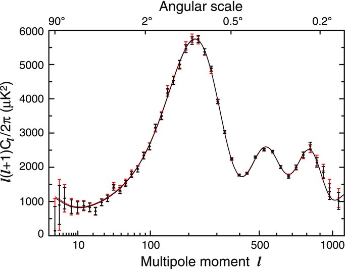
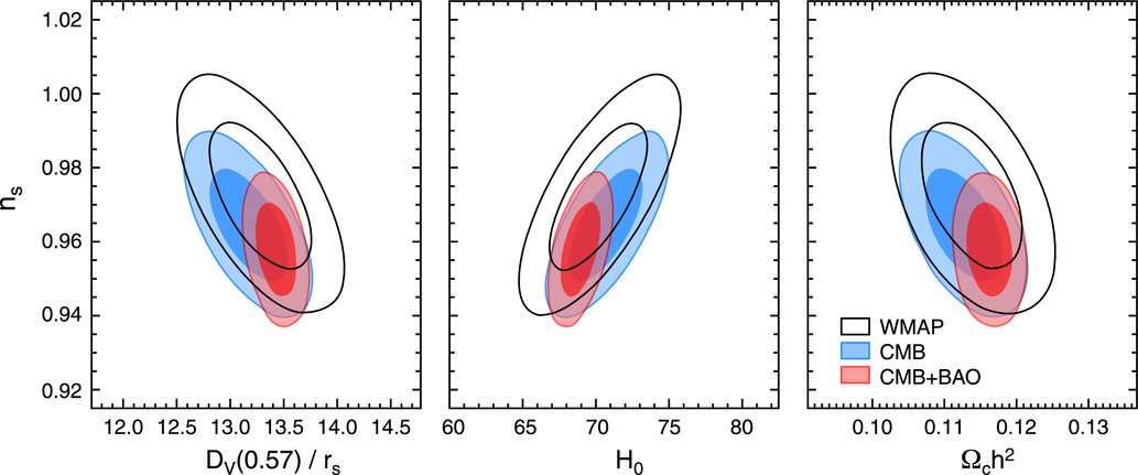
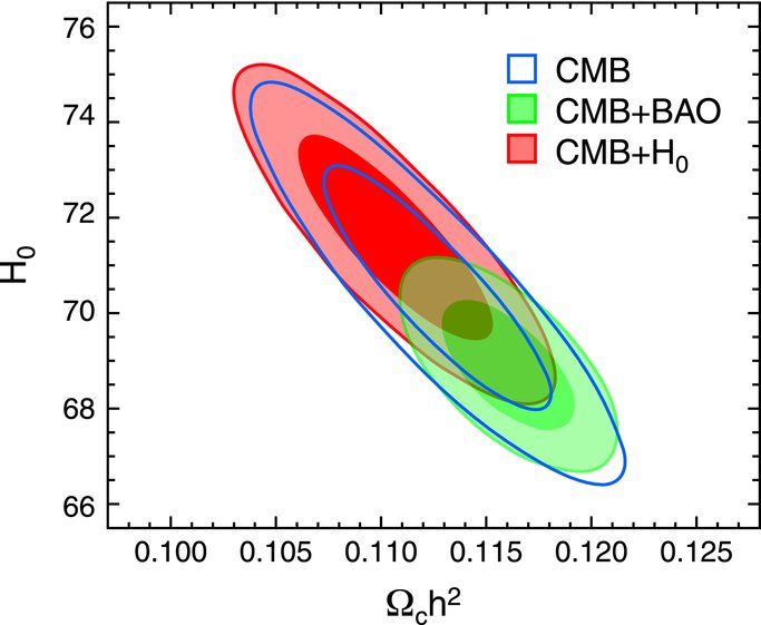