


ABSTRACT
Geometrical (uniform disk) and numerical models were calculated for a set of B-emission (Be) stars observed with the Palomar Testbed Interferometer (PTI). Physical extents have been estimated for the disks of a total of 15 stars via uniform disk models. Our numerical non-LTE models used parameters for the B0, B2, B5, and B8 spectral classes and following the framework laid by previous studies, we have compared them to infrared K-band interferometric observations taken at PTI. This is the first time such an extensive set of Be stars observed with long-baseline interferometry has been analyzed with self-consistent non-LTE numerical disk models.
Export citation and abstract BibTeX RIS
1. INTRODUCTION
B-emission (Be) stars are hot, rapidly rotating main sequence or slightly evolved stars surrounded by gaseous disks. Their visible spectra have at least one hydrogen Balmer emission line (Jaschek et al. 1981). The emission lines need not be continuously present, and a Be star does not lose its classification in the event that the line can no longer be observed (Porter & Rivinius 2003). The general view is that the emission lines arise from the presence of matter which has accumulated around the star due to stellar mass loss. According to Zorec & Briot (1997) the proportion of Be stars among ordinary B stars is at least 17% and is as high as 34% for spectral type B1e. Interestingly, they also find that the frequency of Be stars is independent of luminosity class for the classes V to III. This suggests that Be stars do not represent a specific stage in stellar evolution but that the properties of the star itself and its formation history are responsible for the observational features of this group.
Struve (1931) proposed the existence of disks around a number of stars including γ Cassiopeiae and now it is commonly accepted that disk-like distributions of gas surround Be stars. The study of these disks has been an active area of research for decades but none of the proposed models have been completely successful at explaining the origin or the physical characteristics of the circumstellar disks (Porter & Rivinius 2003). Improvements in instrumentation, especially high resolution interferometry (see, for example, Quirrenbach et al. 1997; Tycner et al. 2005), and the suggestion by Townsend et al. (2004) that Be star rotation rates have been systematically underestimated, have rekindled interest in finding viable models for these systems. Recently, the viscous disk model, originally championed by Lee et al. (1991), has been used successfully to model a number of key observables from Be star systems (see, for example, Carciofi et al. 2012).
A common characteristic that all Be stars appear to share is rapid stellar rotation. For some Be stars their rotational velocity may approach their critical velocity (vcrit) at which material at the equator would be rotationally supported (Townsend et al. 2004). The actual values for their rotation rates are quite contentious, but it is generally accepted that the rates are subcritical ∼0.7vcrit (Porter 1996). Establishing these rotational velocities alongside with the general physical properties of the disk structures is pivotal to our understanding of the processes that give rise to Be star behaviors (Cranmer 2005).
In this study, we concentrate on establishing the physical characteristics of the circumstellar disks associated with these rapidly rotating stars by constraining numerical models with interferometric observations. In particular, we utilize high-angular resolution observations of 16 B-type emission stars that were obtained with the Palomar Testbed Interferometer (PTI) and which resolve the circumstellar structures in the K-band. Our study focuses on the classical Be type stars, however, we included all B-type objects with emission in the archive. For example, β Per is an Algol system, P Cyg is a luminous blue variable (LBV), and some of the other program stars are likely members of binary systems. Nevertheless, we included all of the observations available in this archival set to maximize the number of objects in our study and to provide these observations to the community. Our program stars are listed in Table 1 along with their HD number, spectral type, and any special identifying features.
Table 1. List of Targets
| Target | HD | Spectral Type | N | Obs. Seasons | Distance (pc) | Notes |
|---|---|---|---|---|---|---|
| γ Cas ... | 5394 | B0IVpe | 14 | 2002 | 188 ± 20 | Possible binarya,b,d |
| ϕ Per ... | 10516 | B2Vpe | 245 | 2000–2006 | 220 ± 9.7 | Short-period variability, binaryc,d |
| β Per ... | 19356 | B8V | 25 | 1998–1999 | 28 ± 1 | Algol-type variablee,f |
| ψ Per ... | 22192 | B5Ve | 51 | 2000–2005 | 179 ± 7.04 | Short-period variabilityc,d |
| η Tau ... | 23630 | B7III | 108 | 1998–2001 | 124 ± 6.42 | |
| 28 Tau ... | 23962 | B8IVe | 48 | 2000–2006 | 208 ± 29 | Variabled |
| 48 Per ... | 25940 | B3Ve | 5 | 1999–2002 | 146 ± 3.42 | |
| ζ Tau ... | 37202 | B2IV | 17 | 1998–2005 | 136 ± 15.3 | Variable; non-axisymmetric diskc,d,g |
| ν Gem ... | 45542 | B6IIIe | 3 | 2001 | 167 ± 7.8 | Variabled |
| β CMi ... | 58715 | B8Ve | 10 | 1999–2003 | 50 ± 0.49 | |
| β Lyr ... | 174638 | B7Ve+ | 127 | 1998–2003 | 295 ± 15 | β Lyrae variableh |
| 28 Cyg ... | 191610 | B2.5Ve | 38 | 2000–2001 | 317 ± 23 | |
| P Cyg ... | 193237 | B2pe | 154 | 1998–2002 | 3100 ± 1500 | Luminous blue variablei,j |
| 59 Cyg ... | 200120 | B1.5Vnne | 2 | 2001 | 435 ± 79 | Variabled |
| υ Cyg ... | 202904 | B2Vne | 30 | 1998–2001 | 197 ± 21 | Variablec |
| EW Lac ... | 217050 | B3IVpe | 37 | 2001–2002 | 252 ± 18 | Variablec,d |
Notes. Column 4: N represents the number of squared visibilities obtained at PTI. Column 5: range of observational seasons covered by the observations. Column 6: distance based on Hipparcos parallax (Perryman et al. 1997 for γ Cas; van Leeuwen 2007 for all others). Column 7: distinguishing characteristics of the stars, as applicable and references. aHarmanec et al. (2000). bMiroshnichenko et al. (2002). cHubert & Floquet (1998). dRivinius et al. (2006). eGoodricke (1783). fZavala et al. (2010). gSchaefer et al. (2010). hHarmanec (2002). ide Groot (1969). jBalan et al. (2010).
Download table as: ASCIITypeset image
The results of this study are an extension of a similar observational study by Gies et al. (2007) who observed four Be stars with the CHARA interferometer in the K'-band and obtained very detailed constraints on the disk parameters. The targets in common with Gies et al. (2007) and this study include γ Cassiopeiae, ϕ Persei, and ζ Tauri. Gies et al. (2007) utilized isothermal disk models to obtain very precise disk parameters, while the results presented in this work are based on disk models that enforce self-consistent temperature distributions. In Section 2, we give an overview of our techniques for calibrating and analyzing the observations. We describe the geometrical and numerical modeling procedures we employed to characterize the disks in Section 3. The results of the comparison of our detailed numerical models to the calibrated observations are given in Section 4. Section 5 provides a comparison of our results with other findings and Section 6 summarizes our work.
2. OBSERVATIONS
The interferometric observations used in this study have been acquired at the PTI, located at the Palomar Observatory in California. For a complete description of PTI, the reader is referred to Colavita et al. (1999). The observations used in our analysis were acquired between 1998 and 2006 (see Table 1 for the range of dates associated with each target).
The raw observations have been extracted from the PTI archive, which contain only those observations that meet specific quality standards. For example, observations are assigned grades according to the quality based on observational parameters such as jitter, squared visibility, and photon counts. Furthermore, the criteria for grading the results are based on past performance of the instrument rather than specific limits, thereby giving a more robust assessment of the quality of the observations under consideration.
Data analysis commenced with processing of essentially raw values from the instrument that contains some minor preprocessing and are known as Level 1 (L1) values (Colavita 1999). These values consist of 150 s of integration, averaged over all wavelength channels from 2.0 to 2.4 μm, and include observations of the target and its calibrator stars. For the purpose of our study, we have opted to exclude observations that have piston jitter in excess of 1.50 rad, thereby producing "cleaner" results than what would be obtained without such a restriction.
The calibration of the Be star V2 values is performed by estimating the interferometer system visibility ( ) through observing calibration sources with empirically established point-like angular diameters (van Belle et al. 2008) to estimate the V2 measured by an ideal interferometer at that epoch and then normalizing the raw Be star visibility by
  (Mozurkewich et al. 1991; Boden et al. 1998; van Belle & van Belle 2005). Uncertainties in the system visibility and the calibrated target visibility are inferred from internal scatter among the values in an observation using standard error-propagation calculations (Colavita 1999). Calibrating our point-like calibration objects against each other produced no evidence of systematics, with all objects delivering reduced V2 = 1. PTI's limiting night-to-night measurement error is
  %, the source of which is most likely a combination of effects: uncharacterized atmospheric seeing (in particular, scintillation), detector noise, and other instrumental effects. This measurement error limit is an empirically established floor from the previous study of Boden et al. (1999).
PTI has three baselines, north–west (NW), south–west (SW), and north–south (NS) with lengths 86, 87, and 110 m, respectively. The calibrated observations used in this study were all made with either the NS or NW baselines. The majority of stars in our sample have been observed at these baselines; however, a few had observations on only one. A list of Be stars for which observations have been extracted is given in Table 1. For the 16 targets, a total of more than 900 V2 points have been obtained from the PTI archive and calibrated. The V2 observations for all of our targets are plotted in Figure 1.
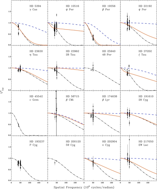
Figure 1. Squared visibility values for the 16 program stars. The UD models fitted to the observations (dash-dotted line) along with UD model representing the star itself based on the adopted stellar diameter (dashed line) are shown. The results based on the hydro-on models with the lowest reduced χ2 are also shown (solid lines).
Download figure:
Standard image High-resolution imageWe note that the formal error bars shown in Figure 1 do not account for all sources of noise. The errors do account quite well for the sources of random noise that can be attributed to photon statistics and calibration errors. However, these formal errors will not account for all sources of atmospheric variations, especially those that are not well tracked by the calibrator star. In other words, if there is atmospheric perturbation of the wavefront on timescales shorter than the cadence of the target–calibrator pairs, then such variations will not be removed during the calibration process nor will they be fully accounted for with the formal error bars. Since many Be stars are known to be variable on a variety of timescales, certainly some of the scatter is a result of this characteristic. The amount of scatter depends on the frequency of such variation, the magnitude of the variability and whether the variability was captured during the time of our observations. Furthermore, since we combine the observations for each star, our calculated disk sizes (see Table 2) and our range of density parameters (see Section 4.3) represent an average over the time that the observations were acquired.
Table 2. Uniform Disk Model Results
| Spectral Group | Target | θ (mas) | θ (AU) |  (θ) (θ) |
|---|---|---|---|---|
| B0 | γ Cas... | 1.66 ± 0.05 | 0.31 ± 0.03 | 10.4 |
| B2 | ϕ Per... | 1.59 ± 0.01 | 0.35 ± 0.02 | 11.7 |
| 48 Per... | 0.73 ± 0.13 | 0.11 ± 0.02 | 1.5 | |
| ζ Tau... | 1.57 ± 0.06 | 0.21 ± 0.03 | 5.86 | |
| 28 Cyg... | 0.574 ± 0.039 | 0.18 ± 0.02 | 1.65 | |
| P Cyga... | 1.45 ± 0.01 | 4.5 ± 2.3 | 2.06 | |
| 59 Cyg... | 0.98 ± 0.09 | 4.5 ± 0.43 | 0.09 | |
| υ Cyg... | 1.14 ± 0.01 | 0.22 ± 0.02 | 4.43 | |
| EW Lac... | 0.981 ± 0.033 | 0.25 ± 0.02 | 1.78 | |
| B5 | ψ Per... | 1.1 ± 0.03 | 0.20 ± 0.01 | 4.49 |
| ν Gem... | 2.78 ± 0.11 | 0.46 ± 0.03 | 0.587 | |
| B8 | β Per (Algol)... | 2.78 ± 0.02 | 0.077 ± 0.003 | 3.07 |
| η Tau... | 0.712 ± 0.011 | 0.088 ± 0.005 | 0.71 | |
| 28 Tau... | 1.04 ± 0.02 | 0.22 ± 0.03 | 1.47 | |
| β CMi... | 0.719 ± 0.323 | 0.036 ± 0.016 | 1.16 | |
| β Lyr... | 0.584 ± 0.02 | 0.17 ± 0.01 | 1.42 | |
Notes. Column 3: size of uniform disk (UD) model in milli-arcseconds. Column 4: size of UD in astronomical units, based on the Hipparcos distances in Table 1. Column 5:  errors estimated from the UD modeling routine and reduced by the number of available observations per star.
aSystem possesses spherical wind structure.
errors estimated from the UD modeling routine and reduced by the number of available observations per star.
aSystem possesses spherical wind structure.
Download table as: ASCIITypeset image
3. METHODOLOGY
3.1. Uniform Disk Modeling
A common first approximation technique for determining the physical extent of the circumstellar regions of Be stars is the uniform disk (UD) model. The UD model, fitted to the interferometric observations in the K-band, assumes that the central star and the surrounding disk can be represented by a circularly symmetric and uniformly illuminated region on the sky. UD fits were performed for all stars for which there were sufficient number of calibrated observations and the resulting angular diameters are listed in Table 2. We used updated Hipparcos parallax measurements from van Leeuwen (2007) for all of our program stars with the exception of γ Cas which did not have an updated parallax. For this star we used the Perryman et al. (1997) measurement. Using these measurements we calculated the distance to each source (see Table 1), and converted the angular sizes in Column 3 of Table 2 to physical dimensions in Column 4. The fifth column of Table 2 lists the reduced  values estimated from the UD modeling routine.
The UD modeling represents a good first-order approximation and is commonly used as a model of choice, especially if the quantity of observations is limited or a simple (and single) parametric description of the circumstellar structure is desired. Nonetheless, it should be noted that the estimated disk sizes are dependent on the functional form of the adopted model and adopting a different geometrical model for the disk will produce different disk sizes. Furthermore, a UD model assumes that the disk and the central star can be approximated with a single uniform surface intensity across the K-band. Of course, a more realistic model would treat the central star and surrounding disk independently, necessitating a different approach to modeling.
In addition to the UD modeling, described above, we also fit our program stars with elliptical disks (ED) to check for deviations from circular symmetry on the plane of the sky. See the paper by Tycner et al. (2006) for details about ED fits. We report our findings below in Section 4.
3.2. Numerical Disk Modeling
The basic model for a circumstellar disk of a Be star represented by a geometrically thin, equatorial disk, heated by the photoionizing radiation field of the central star was championed by Poeckert & Marlborough (1978) and since then has become a highly cited model. An extension of the model to a non-UD temperature structure based on radiative equilibrium was first obtained by Millar & Marlborough (1998). The numerical disk models presented in this study are computed using the latest version of this disk model, which enforces radiative equilibrium and vertical hydrostatic equilibrium to obtain the disk temperature structure (Sigut & Jones 2007; Sigut et al. 2009). The numerical code (which we refer to as BEDISK code) has been successfully used to interpret a wide range of Be star observables, from interferometric visibilities (Jones et al. 2008; Tycner et al. 2008) to hydrogen line profiles (Silaj et al. 2010) and infrared line fluxes (Jones et al. 2009).
The disk modeling routine, BEDISK, as developed by Sigut & Jones (2007) provides a more physical representation of the star-plus-disk system. Notably, a distinction is made between the intensity of the central star and that of the disk. The central star is represented by a synthetic spectrum chosen from the grid of synthetic model atmospheres of Kurucz (1993), selected based on the Teff and log (g) of the central star. The disk is modeled with a power law density grid as described by

where ρ0 is the density of the disk at the stellar surface, n is the power law exponent, R is the distance from the stellar rotation axis (while R* is the stellar radius), Z is distance in the direction parallel to the star's axis of rotation (and perpendicular to the disk), and H is the vertical scale height, defined as
where
In Equation (3), G is the gravitational constant, M* is the mass of the central star, μ0 refers to the mean molecular weight of the circumstellar material, mH is the atomic mass of hydrogen, k is the Boltzmann constant, and T0 is an assumed isothermal temperature for the disk (which is used only to calculate the disk scale height in Equation (1)). Assuming a constant temperature irrespective of the vertical height Z in this manner allows radiatively balanced models to be generated, although the vertical density distribution is not exactly consistent with the calculated temperature distribution (we refer to these models as "hydro-off"). However, Sigut et al. (2009) has described how BEDISK code can also self-consistently solve for the vertical temperature and density structure of the disk while enforcing vertical hydrostatic equilibrium. In this case, the vertical density structure no longer has the analytic form of Equation (1), although the radial power-law drop-off is still assumed (see Sigut et al. 2009, for more details). We refer to the models generated with the vertical hydrostatic equilibrium enforced as "hydro-on" models.
An important aspect of BEDISK is its use of solar chemical composition. Earlier codes neglected the metallicity of the disk material, given that the disks are obviously composed predominantly of hydrogen. However, heavier elements contribute to the heating and cooling processes within the disk and therefore affect both the thermal structure of the disk and the intensities of its emission lines (Jones et al. 2004). Although Be stars are found in both lower- and higher-metallicity environments, with lower metallicity showing higher prevalence of the Be phenomenon (McSwain & Gies 2005; Martayan et al. 2010), we opt to model the stars in this study at the solar chemical composition.
The models presented here utilized an 84 by 50 grid, meaning the grid consists of 84 radial rings starting at the stellar photosphere, where at each radial location calculations are performed at 50 steps above the mid-plane (mirror symmetry is assumed for the region below the mid-plane). Figure 2 shows the computation grid in the disk as function of R and Z. The output generated by the BEDISK code is in the form of spectral energy distributions, which were used to construct synthetic images. The UD modeling assumed circular symmetry and we extend this assumption to our thermal disk models. However, it is clear that some stars will neither be viewed pole-on, nor might their disks be circularly symmetric. For example, the disk of ζ Tauri (HD 37202) is known to be asymmetric and viewed at a non-zero angle of incidence (Quirrenbach et al. 1997; Vakili et al. 1998; Tycner et al. 2004; Carciofi et al. 2009). However, because the quantity of interferometric values for most of our sources is quite small and in some cases we only have observations from one baseline orientation, reliable determination of deviation from circular symmetry is not possible. Therefore, for the purpose of determining the general physical characteristics of the disks, as opposed to detailed geometrical properties, we neglect the effects of projection and any deviations from circular symmetry in our analysis and instead approximate the disks with circularly symmetric models seen pole-on.
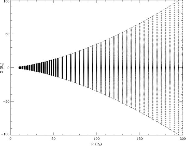
Figure 2. Computational grid throughout the disk as a function of R and Z adopted for this investigation.
Download figure:
Standard image High-resolution imageFollowing the procedure outlined in Tycner et al. (2008) for comparing synthetic images to interferometric observations, we compared the synthetic images from BEDISK to the squared visibilities for each of the 16 sources. We used a χ2 statistic as a measure of goodness-of-fit to find a range of n and ρ0 values that best represent the characteristics of the Be star disk.
The use of circularly symmetric (or pole-on) images for the analysis of the PTI observations does require some further justification. To this end, we have used the BERAY code of Sigut (2011) to construct images of some of our model disks for a range of inclination angles. The BERAY code uses as input the disk temperature and density structure from a BEDISK solution to solve the radiative transfer equation along a series of rays through the Be star-plus-disk system. The non-LTE level populations computed by BEDISK are used to construct the gas opacity and emissivity. Rays that terminate on the stellar surface use a model photospheric intensity (appropriate for the adopted Teff and log (g) for the star) for the boundary condition at the start of the ray. Rays that pass through the disk assume no incident radiation. Thus BERAY produces monochromatic images of the Be star system on the sky which can be used to evaluate how serious an error is made by analyzing the PTI sample with the circular, zero-inclination images produced by BEDISK.
Figure 3 shows the results for a model of the Be star γ Cas with disk density parameters n = 3.5 and ρ0 = 1.0 × 10⁻¹⁰ g cm−3. An outer disk radius of Rd = 12 R* was assumed, and the images were produced in the K band (2.179 μm) with a resolution on the sky of 0.05 R*. The model was assumed to be viewed at a distance of 188 pc, the Hipparcos catalog distance for γ Cas (Perryman et al. 1997). Images were produced for viewing inclinations of 5°, 45°, and 60°. To compute the interferometric visibilities, the images were summed along the minor axis of the disk, and the resultant one-dimensional images (along the major axis) were discrete Fourier transformed (DFT) to produce the corresponding visibilities. The major axis was selected in order to use the largest spatial scale present in each image, which gives the largest departures from unity in the corresponding visibilities (where a visibility of 1 corresponds to an unresolved point source). Hence this approach is representative of what happens when the disk is fully resolved by the observations. The left panel of Figure 3 shows the minor-axis summed, one-dimensional images, and the right panel the DFT of these images. As can be seen from the figure, the effect of inclination is quite small; the visibilities at 50 Mλ, the maximal spatial frequency for the 110 m baseline of PTI in the K band, differ by about ±10%. This difference is likely well within our observational uncertainties. Thus the signal is mainly sensitive to the bulk properties of the disk gas (to within the limits shown) and not to the geometry along the unresolved dimension. For this reason, we are confident that the uncertainties introduced by use of the circular, pole-on image of BEDISK to analyze our sample of Be stars in a uniform manner are entirely commensurate with the PTI data quality.

Figure 3. Left panel: major axis, summed intensity as a function of offset from the center of the star (in milli-arcseconds) for the γ Cas model seen at three inclination angles. The profiles are normalized to unit area. The disk model assumed n = 3.5, ρ0 = 1.0 × 10⁻¹⁰ g cm−3, and Rd = 12 R*. Right panel: the corresponding discrete Fourier transforms expressed as visibility vs. spatial frequency (in units of 106 cycles rad−1).
Download figure:
Standard image High-resolution image4. RESULTS
4.1. Uniform Disks
Figure 1 shows the observed squared visibility versus spatial frequency for the 16 stars in our sample. The model curves for the circularly symmetric UD results, with the angular disk sizes listed in Table 2, are also shown. The stars listed in Table 2 have been divided into groups based on spectral type for ease of comparison with the results from the next section, which separate all the targets into one out of four groups. The groups divide the spectral range B0–B8 into four groups with γ Cas as the only B0 star; B1.5 to B3 stars in the second group, B5 to B6 stars in the third group, and all remaining stars (B7 to B8) in the fourth group.
Overall the UD fits model the observations well with a few exceptions. The targets that showed relatively low quality fits, as determined based on the reduced χ2 values listed in Table 2, were γ Cas, ϕ Per, ζ Tau, υ Cyg, ψ Per, and β Per. We attribute these low quality fits to a combination of non-pole geometry for γ Cas (see Section 4.2), variations from axisymmetry, variability, and at least in the last case to a possible signature of a binary. However, as stated previously, since our observations cover only very limited range of spatial frequencies and we have very small number of values in each of the observing seasons we choose to average these effects by simply fitting a single circularly symmetric model. We believe that such a simple and single parametric description of the interferometric signature is still useful to describe the most general property of the emitting region, i.e., its angular extent on the sky.
4.2. Elliptical Disks
In order to validate our assumption of the assumed circular symmetry for the circumstellar disks we fit the observed squared visibilities shown in Figure 2 with elliptical UD models. The fitting procedure followed the same modeling approach as outlined in Section 4 of Tycner et al. (2006) where the model for the circumstellar disk can be represented by an elliptical UD with an axial ratio r defined as the ratio of the minor to major axis (i.e., an axial ratio of unity represents a circularly symmetric disk).
For the stars, β Per, ψ Per, η Tau, 28 Tau, β Lyr, and P Cyg we find axial ratios close to unity supporting the fact that our assumption of circular symmetry is appropriate. For these stars their ratios range from a minimum of 0.60 ± 0.05 to a maximum of 0.75 ± 0.04 with a mean and standard deviation of 0.73 ± 0.08, respectively. For ϕ Per, 48 Per, ζ Tau, β CMi, 28 Cyg, υ Cyg, and EW Lac the errors are very large and we conclude that the elliptical UD fit simply fails to converge to a valid solution with a statistically meaningful axial ratio (i.e., we fail to detect axial flattening in these systems).
For 48 Per, ν Gem, and 59 Cyg there were not enough observations to justify an elliptical model fit (see Table 4) so we did not include these targets in our modeling. γ Cas with an axial ratio of 0.30 ± 0.04 is the only target for which our elliptical UD modeling indicates significant ellipticity on the plane of the sky. Therefore, with a possible exception in the case of γ Cas, we proceed with our numerical models under the assumption of circular symmetry and assume that any minor deviations from circular symmetry will average out in the final results and can be ignored for the purpose of our analysis.
4.3. Disk Density Models
4.3.1. Spectral Group B0
We begin our analysis with γ Cas, which is considered an archetypal Be star and as such is particularly well studied. However, observations show characteristics that are atypical for Be stars. For example, it exhibits unusual X-ray behavior and is probably a member of a binary system (Smith et al. 2004; Miroshnichenko et al. 2002). Nonetheless, other studies of γ Cas are widely available for comparison and for that reason it is a good starting point. The total (n, ρ0) grid utilized for the hydro-off models ranged from 1.0 < n < 6.6 and 3.0 × 10⁻¹¹ < ρo < 5.0 × 10⁻⁹ g cm−3 and consisted of 283 models. The grid utilized for the hydro-on models was slightly different ranging from 0.1 < n < 6.6 and 7.0 × 10⁻¹² < ρo < 3.0 × 10⁻⁸ g cm−3 and totaled 290 models. We note that the (n, ρ0) grid is only approximately uniformly sampled with a coarser grid at the extremes of the parameters. Second, models were not produced for all combinations of n and ρo within this range. For example, models were required to be dense enough to produce emission but not so dense that gas became totally neutral. Generally, for increasing values of n (corresponding to faster density fall-off with increasing distance from the star) higher values of ρo are required. A comparison between models produced with and without hydrostatic equilibrium enforcement, revealed noticeable differences especially in the highest density models. Basically, if the disks are dense enough to develop a cool region in the equatorial plane, the hydrostatic enforced disks have material concentrated in a thinner volume toward the plane (Sigut et al. 2009). These differences in density distribution lead to changes in the thermal structure of the disk.
Figures 4 and 5 give an example of the density and temperature distribution, respectively, for a very dense disk corresponding to the model with n = 4.8 and ρ0 = 1.0 × 10⁻⁹ g cm−3 for γ Cas. Notice in Figure 4 that the region of highest density is narrower in vertical extent nearest the star with hydro-on compared with the hydro-off case. For example, compare the density that corresponds to ∼10−12 g cm−3 (in yellow) at a distance of ∼20 R☉. In the case of hydro-on, the vertical extent of this volume of gas is ∼20% narrower. Similarly, Figure 5 shows that near the star in the equatorial plane the vertical extent of the cooler region is clearly compressed with hydro-on compared to hydro-off. For example, at a distance of ∼40 R☉ the cool portion of the gas (in blue) corresponding to ∼6000 K is nearly twice in the vertical extent with hydro-off. Figure 5 also shows that the overall disk temperature is hotter in the hydro-off case, which can be attributed to a larger quantity of gas at greater distances from the equatorial plane that has direct line of sight of the source of the ionizing radiation field originating at the stellar photosphere.
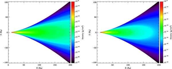
Figure 4. Computed density structures for γ Cas with n = 4.8 and ρ0 = 1.0 × 10⁻⁹ g cm−3, with (left panel) and without (right panel) hydrostatic equilibrium enforcement.
Download figure:
Standard image High-resolution image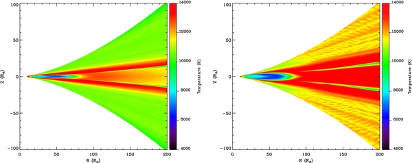
Figure 5. Computed temperature structures for γ Cas with n = 4.8 and ρ0 = 1.0 × 10⁻⁹ g cm−3, with (left panel) and without (right panel) hydrostatic equilibrium enforcement.
Download figure:
Standard image High-resolution image
There is a subtle point to keep in mind when comparing the hydro-off and hydro-on cases. For the hydro-off models the disk density in the vertical direction is set a priori based on a fixed value for the disk temperature, T0, in Equation (3). The value of T0 used in this study for γ Cas is 13,500 K and is based on typical density-weighted average temperature of the disk from our models, whereas for the hydro-on case the density is determined from the hydrostatic solution constrained by the value of n and ρ0. The implication for each of these constraints is that the mass of the disk with the same value of n and ρ0 is different in the hydro-on and hydro-off cases. As a result, hydro-on models have a total disk mass ∼20% less than the hydro-off case (Sigut et al. 2009). This could certainly account for the larger average disk temperature for the hydro-off model in Figure 5 because there is more material distributed out of the plane of the disk where it can be more easily ionized by the stellar radiation field.
We have adopted both the hydro-on and hydro-off models for γ Cas. The infrared excesses are believed to originate in the densest region of the disk near the star and in and near the equatorial plane (Touhami et al. 2010). Therefore, since the hydro-on models provide a self-consistent density and temperature distribution, especially important for the densest regions, the hydro-on models are expected to provide a more realistic representation of the physical conditions in the dense gas. However, since many of the previous studies that used the code BEDISK did not employ the hydro-on case we have also presented the results for γ Cas with hydro-off for comparison. We also note that for early-type Be stars, Sigut et al. (2009) found that differences in predicted infrared excesses from hydro-on and hydro-off were quite small for reasonable values of To. Rows 1 and 2 of Table 4 give our results for γ Cas for the hydro-off and hydro-on cases, respectively. The best fits were obtained from models corresponding to a range in reduced χ2 from the minimum value to the minimum plus 10%. The minimum, maximum, and mean values for both n and ρo for the subset of models corresponding to this range in reduced χ2 are also provided in Table 4. The numerical model for γ Cas (HD 5394) with the minimum reduced χ2 for the hydro-on case is displayed in Figure 1 with a solid line.
We note that our range of best-fitting model parameters for γ Cas, and our other program stars, each represent an average set of parameters for the density over the time the observations were collected.
4.3.2. Spectral Group B2
Five stars in Table 1 are of spectral class B2; an additional four are of adequately similar spectral class (B1.5, B2.5, B3) that the B2 spectral class parameters can be used to approximate their characteristics. The stellar parameters used to generate the models were taken or estimated from Cox (2000) and are given in Table 3. As previously mentioned, the parameters represent average estimates for a given stellar class and are not an exact match for each star's characteristics. These stars are shown grouped together in Tables 2 and 4. The hydro-on case was used to generate models of all the program stars in this group. In total, for this group of stars 220 models were constructed with 1.0 < n < 6.0 and 1.0 × 10⁻¹² < ρo < 1.0 × 10⁻⁸ g cm−3. The subset of models corresponding to a range in reduced χ2 values from the minimum to the minimum plus 10% are shown in Table 4. For each of these stars, the solid line in Figure 1 corresponds to the hydro-on model with the minimum χ2 value.
Table 3. Adopted Stellar Parameters
| Spectral Type | Stellar Radius (R☉) | Stellar Mass (M☉) | Teff (103 K) |
|---|---|---|---|
| B0... | 10.0 | 17.0 | 25.0 |
| B2... | 5.7 | 10.9 | 20.9 |
| B5... | 3.9 | 5.9 | 15.2 |
| B8... | 3.0 | 3.8 | 11.4 |
Notes. All stellar models assumed log g = 4.0 for the central star. Stellar parameters for the B0 the spectral class were taken from Millar & Marlborough (1998). Parameters for B2, B5, and B8 were adapted from Cox (2000).
Download table as: ASCIITypeset image
Table 4. Detailed Model Best Fits
| Target | Reduced χ2 | n | ρo (g cm−3) | |||||
|---|---|---|---|---|---|---|---|---|
| Min | Max | Min | Max | Mean | Min | Max | Mean | |
| γ Casa | 11.24 | 12.35 | 2.8 | 6.2 | 3.95 | 3.0e−11 | 5.0e−09 | 7.67e−10 |
| γ Casb | 13.54 | 14.83 | 2.1 | 6.5 | 4.13 | 7.0e−12 | 3.0e−08 | 2.25e−09 |
| ϕ Per | 6.81 | 7.16 | 1.5 | 2.0 | 1.83 | 2.0e−12 | 3.0e−11 | 1.73e−11 |
| 48 Perc | ⋅⋅⋅ | ⋅⋅⋅ | ⋅⋅⋅ | ⋅⋅⋅ | ⋅⋅⋅ | ⋅⋅⋅ | ⋅⋅⋅ | ⋅⋅⋅ |
| ζ Tau | 4.56 | 5.00 | 2.0 | 2.5 | 2.10 | 7.0e−12 | 7.0e−12 | 2.08e−11 |
| 28 Cyg | 1.70 | 1.85 | 2.0 | 6.0 | 4.35 | 3.0e−12 | 1.0e−08 | 2.31e−09 |
| P Cyg | 37.31 | 40.95 | 1.0 | 1.5 | 1.40 | 1.0e−12 | 1.0e−11 | 7.00e−12 |
| 59 Cygc | ⋅⋅⋅ | ⋅⋅⋅ | ⋅⋅⋅ | ⋅⋅⋅ | ⋅⋅⋅ | ⋅⋅⋅ | ⋅⋅⋅ | ⋅⋅⋅ |
| υ Cyg | 4.58 | 5.01 | 2.0 | 4.0 | 2.80 | 8.0e−12 | 1.0e−08 | 1.51e−09 |
| EW Lac | 1.99 | 2.10 | 3.5 | 4.0 | 3.88 | 2.0e−09 | 1.0e−08 | 7.25e−09 |
| ψ Per | 5.03 | 5.53 | 1.2 | 2.5 | 1.78 | 4.0e−11 | 9.0e−09 | 8.18e−10 |
| ν Gemc | ⋅⋅⋅ | ⋅⋅⋅ | ⋅⋅⋅ | ⋅⋅⋅ | ⋅⋅⋅ | ⋅⋅⋅ | ⋅⋅⋅ | ⋅⋅⋅ |
| β Per | 12.65 | ⋅⋅⋅ | 3.0 | ⋅⋅⋅ | ⋅⋅⋅ | 8.0e−09 | ⋅⋅⋅ | ⋅⋅⋅ |
| η Tau | 0.96 | 1.03 | 3.0 | 3.0 | 3.0 | 8.0e−09 | 1.0e−08 | 9.00e−09 |
| 28 Tau | 18.70 | 20.51 | 1.0 | 6.0 | 3.42 | 1.0e−12 | 1.0e−08 | 1.58e−09 |
| β CMi | 1.30 | 1.40 | 1.0 | 5.0 | 3.24 | 1.0e−12 | 5.0e−10 | 6.26e−11 |
| β Lyr | 4.50 | 4.95 | 1.0 | 6.0 | 3.32 | 1.0e−12 | 1.0e−08 | 2.70e−09 |
Notes. aResults for the hydro-off models. bResults for the hydro-on models. cFor these three stars there was not enough observations to justify a model fit.
Download table as: ASCIITypeset image
Of all targets, ϕ Per (HD 10516, B2Vpe) has the largest number of calibrated observations (see Table 1). The best-fit models have a range in reduced χ2 from 6.81 to 7.16, indicating that the model fit is not especially good. The observations plotted in Figure 1 for ϕ Per (HD 10516) show that despite the large number of observations, much of it is centered approximately on two values of the spatial frequency which limits the effectiveness of the observations to provide strong model constraints.
The asymmetric disk (Quirrenbach et al. 1997; Vakili et al. 1998) of ζ Tau (HD 37202, B2IV), was best fit by a set of models having smaller values for n. The model corresponding to the lowest value for reduced χ2 = 2.0 has n = 2.0 and ρ0 = 7.0 × 10⁻¹² g cm−3. We note that this fit was of higher quality than that of ϕ Per, with reduced χ2 = 4.56.
P Cyg (HD 193237, B2pe) differs considerably from the other stars in the catalog. It belongs to a class of stars referred to as LBV stars, which are evolved, massive, and highly luminous stars that demonstrate some type of instability. P Cyg has experienced violent mass-loss events (see Smith & Hartigan 2006) and as a result our disk models were not expected to fit the more spherically distributed circumstellar material. Consequently, the model fit failed as indicated by the reduced χ2 values; the minimum value is 37. Therefore, we have not plotted the detailed model best fit in Figure 1 and only the observations and UD model are shown.
The best reduced χ2 fits within this group of stars are for 28 Cyg (HD 191610, B2.5Ve) and EW Lac (HD 217050, B3IVpe). Interestingly these stars are associated with early-type spectral classes, specifically B2.5 and B3. It is also interesting to note that these two stars all had best-fit models that correspond to n of 2.0 or greater. There are three other stars in this group: 48 Per (HD 25940, B3Ve), 59 Cyg (HD 200120, B2Vne), and υ Cyg (HD 202904, B3IVpe). 48 Per and 59 Cyg had too few observations to constrain our detailed models (see Table 1) and as a result further modeling was not completed. Therefore, Figure 1 shows only the observations and UD fit for this star. Also, υ Cyg did not have good reduced χ2 values and further discussion is provided in Section 5.
4.3.3. Spectral Group B5
Another set of models using the parameters for spectral class B5 was generated and compared to the observations for ψ Per (HD 22192, B5Ve). In total, there were 285 models constructed with 1.2 < n < 6.0 and 6.0 × 10⁻¹² < ρo < 1.0 × 10⁻⁸ g cm−3. The adopted stellar parameters and the results for the subset of the preferred models are listed in Tables 3 and 4, respectively, for the star ψ Per. For ν Gem there were only three observations in our archival set, therefore, analogous to the stars 48 Per and 59 Cyg, only the observations and UD fit are presented in Figure 1.
4.3.4. Spectral Group B8
Finally, a set of models were produced for the five remaining late-type stars using the B8 stellar parameters listed in Table 3 over a range of 1.0 < n < 6.0 and 1.0 × 10⁻¹² < ρo < 1.0 × 10⁻⁸ g cm−3. Again, these stars are shown grouped together by the horizontal lines in Tables 2 and 4. Table 4 provides the range of model parameters for our preferred subset of models and the solid line in Figure 1 shows the model corresponding to the minimum reduced χ2.
For β Lyr (HD 174638, B7e+), although the quality of the fit was relatively good with a minimum reduced χ2 of 4.5, it needs to be emphasized that this star is an interacting binary (Schmitt et al. 2009; Zhao et al. 2008). Therefore, the results of this study need to be approached cautiously and further analysis is needed to get a complete picture of this system. In fact, the subset of models that correspond to within 10% of the minimum reduced χ2 which span the entire range of n investigated. For β Per (HD 19356, B8V), a well known Algol-type eclipsing binary, we were not able to find a good fit as indicated by the minimum reduced χ2 of 12.65. For the other stars in this spectral range, a rather poor fit was obtained for 28 Tau (HD 23962, B8IVe), while good fits were found for η Tau (HD 23630, B7III) and β CMi (HD 58715, B8Ve).
5. DISCUSSION
Our study includes objects in common with other work presented in the literature and it is illuminating to compare the results presented here with other investigations. Similar work was performed by Gies et al. (2007) using the CHARA array to observe Be stars in the K'-band. We have three stars in common with their study: γ Cas, ϕ Per, and ζ Tau. For γ Cas we obtained quite a large range in model parameters for our subset of best-fit models. Gies et al. (2007) considered two different models in their analysis, a single star model and a binary system. They obtained a value for n of 2.70 and 2.65 and ρo of 7.24 × 10⁻¹¹ g cm−3 and 6.61 × 10⁻¹¹ g cm−3 for the single and binary solutions, respectively. These values fall within the range of our best-fit subset of models for γ Cas. However, Table 4 shows that for γ Cas, with both hydro-off and hydro-on, the set of preferred models is quite large and consists of a large range in both n and ρo. This could be due to several factors. The χ2 values indicate that the fit is not ideal. The assumption that the disk is symmetric about the mid-plane may not be fully appropriate for γ Cas. We note that the fits obtained by Gies et al. (2007) with  of 24.3 and 24.0 are also not of high quality which may be further proof that an axisymmetric disk is not a good representation for γ Cas. Also recall that we found some evidence for ellipticity for γ Cas (see Section 4.2). In addition, as shown in Figure 1 most of the observations were obtained at only a few spatial frequencies which places limits on how well the numerical models can be constrained.
For ϕ Per our detailed model fits were much better and the agreement with Gies et al. (2007) is excellent. Gies et al. (2007) obtained a value for n of 1.80 and 1.76 and ρo of 1.20 × 10⁻¹¹ g cm−3 and 1.05 × 10⁻¹¹ g cm−3 for the single and binary solutions, respectively. We find 1.5 < n < 2.0 and 2.0 × 10⁻¹² < ρo < 3.0 × 10⁻¹¹ g cm−3 for this star. It is interesting that we both obtain a small value of n based on the infrared observations. This suggests that the density distribution, at least near the star, falls off quite slowly.
Finally for ζ Tau, Gies et al. (2007) obtained values for n of 3.14 and 3.19 and ρo of 1.95 × 10⁻¹⁰ g cm−3 and 1.86 × 10⁻¹⁰ g cm−3 for the single and binary solutions, respectively. We find smaller values, 2.0 < n < 2.5, and correspondingly smaller values of ρo (see Table 4).
For the other early-type stars reasonable fits were obtained for program stars with the exception of 48 Per which we were unable to model due to insufficient observations.
We also have a number of stars in common with the work of Waters et al. (1987) who used simple disk models to study the far infrared characteristics using the Infrared Astronomical Satellite. Although the observations were obtained at a different epoch, it is interesting to compare our results to theirs. Waters et al. (1987) obtained 2 < n < 3.5 for their range of the power law fall-off. Their values for ρo generally agree with our findings, but Waters et al. (1987) values are typically at the lower end of our range. Perhaps this is not surprising because Waters et al. (1987) uses a constant opening angle of 15° for their disk models with the density at a given radial distance remaining constant along radial arcs above and below the equatorial plane. Recall that in our models, the disk density falls off exponentially perpendicular to the equatorial plane. Therefore, we require higher values of ρo to have an equivalent amount of gas within the disk.
6. CONCLUSIONS
We have assembled a collection of UD and numerical disk models for comparison with K-band interferometric observations for 16 Be stars spanning spectral types from B0 to B8. UD models for 16 targets were fitted to K-band archival observations from the PTI. We also determined the disk density distribution using numerical models constructed with the non-LTE radiative code BEDISK (Sigut & Jones 2007) for the remaining 15 stars. Our collection of numerical models has the distinction of being thermally balanced in addition to having been generated with solar chemical composition. This analysis allowed us to select a range of preferred model parameters by a comparison to the interferometric observations based on standard χ2 tests for all but 3 of the 15 stars (see Table 4). We present a range of best-fitting model parameters for our program stars, representing the average density over the time the observations were collected for each star. Due to the intrinsic variability of Be stars and some of our other program stars, our range of best-fit density parameters may only be appropriate for the time over which the PTI observations were obtained.
For P Cyg (HD 193237), which possesses a spherical wind, our disk model fits failed and for the three other stars, 48 Per (HD 25940), 59 Cyg (HD 200120), and ν Gem (HD 45542), there were insufficient values to constrain our detailed models.
By combining the results from all our targets, we find best-fit models corresponding to model input parameters that ranged substantially in value with 1.0 < n < 6.5 and 1.0 × 10⁻¹² < ρo < 3.0 × 10−08 g cm−3. A simple average value of n over all of our program stars for our preferred models is 3.03 ± 0.94. This result is in good agreement with other investigations of Be star disks in the infrared regime (Waters et al. 1987; Gies et al. 2007).
Silaj et al. (2010) also used the BEDISK code to construct Hα profiles for comparison with observations of 69 Be stars. Although the Hα emitting region samples a larger volume of the disk, it is instructive to compare our results with Silaj et al. (2010). Analogous to our findings, Silaj et al. (2010) determined that a large range of n and ρo was required to produce suitable profiles for their program stars. Interestingly, their values for n were strongly peaked at 3.5 (see Silaj et al. 2010, Figure 7). This value agrees quite well with our simple average of n = 3.03 from our subset of preferred models.
For some of our program stars we obtain preferred models that include upper limits of ρo that are quite large. In fact, as discussed in Cranmer (2005), the largest values coincide with typical values associated with stellar photospheres. These large densities near the star in the equatorial region are consistent with the suggestion by Koubsky et al. (1997) that Be star disks begin as an optically thick extension of the star that eventually develops into a disk. Future work will be necessary to determine the generality of this statement.
This material is based upon work supported by the National Aeronautics and Space Administration under grant No. NNX08AQ24A. The Palomar Testbed Interferometer is operated by the NASA Exoplanet Science Institute and the PTI collaboration and was constructed with funds from the Jet Propulsion Laboratory, Caltech, as provided by the National Aeronautics and Space Administration. This research has made use of the SIMBAD database, operated at CDS, Strasbourg, France. B.J.G. acknowledges support from Central Michigan University. This research has made use of services produced by the NASA Exoplanet Science Institute at the California Institute of Technology. This work is supported by the Canadian Natural Sciences and Engineering Research Council through Discovery Grants to T.A.A.S. and C.E.J.
Facility: PO:PTI - Palomar Testbed Interferometer