


ABSTRACT
Magnitude differences obtained from speckle imaging are used in combination with other data in the literature to place the components of binary star systems on the H–R diagram. Isochrones are compared with the positions obtained, and a best-fit isochrone is determined for each system, yielding both masses of the components as well as an age range consistent with the system parameters. Seventeen systems are studied, 12 of which were observed with the 0.6 m Lowell-Tololo Telescope at Cerro Tololo Inter-American Observatory and six of which were observed with the WIYN 3.5 m Telescope (The WIYN Observatory is a joint facility of the University of Wisconsin-Madison, Indiana University, Yale University, and the National Optical Astronomy Observatories) at Kitt Peak. One system was observed from both sites. In comparing photometric masses to mass information from orbit determinations, we find that the photometric masses agree very well with the dynamical masses, and are generally more precise. For three systems, no dynamical masses exist at present, and therefore the photometrically determined values are the first mass estimates derived for these components.
Export citation and abstract BibTeX RIS
1. INTRODUCTION
Since its inception in the 1970s, speckle interferometry has been an important technique for determining high-quality orbits of visual binary stars. The outstanding astrometric precision of the technique in particular has made it possible to collect valuable data even from small-aperture telescopes, most notably the 0.66 m refractor at the U.S. Naval Observatory in Washington, DC; see Mason et al. (2007) and references therein. Our group has also done a substantial amount of small-aperture speckle interferometry, mainly in the Southern Hemisphere, from both the 0.76 m telescope at El Leoncito, Argentina (Horch et al. 1996, 2006b) and 0.60 m telescopes at Las Campanas and Cerro Tololo, Chile, e.g., Horch et al. (2006a) and references therein. We have also contributed a substantial number of measures from the WIYN 3.5 m Telescope, the most recent group of which is detailed in Horch et al. (2008).
Photometric information has traditionally been more difficult to obtain from speckle interferometry, though this situation has improved in recent years. For example, magnitude difference measures of subarcsecond binaries obtained with the RIT-Yale Tip-Tilt Speckle Imager (RYTSI) at the WIYN 3.5 m Telescope have an average precision of 0.10 mag per two-minute observation (Horch et al. 2008). RYTSI uses a large-format CCD detector as the image capture device, as detailed in Meyer et al. (2006). At smaller apertures, CCD-based speckle photometry has shown no significant systematic deviations from space-based measures, however, measurement precision is poorer compared to larger-aperture work. In the observations described above at Las Campanas and Cerro Tololo (where a CCD was again used to image the speckle patterns), the uncertainty per two-minute observation is 0.15–0.18 mag for typical observing conditions. A color formed from two such observations in two different filters would of course be even more uncertain.
Nonetheless, with repeated observations of a binary using a small telescope, these uncertainties can in theory be brought down to the point where meaningful comparisons with stellar structure and evolution calculations can be made. In addition, when using a smaller telescope, the effects of atmospheric dispersion are less evident on individual speckles and therefore a wider filter can be used. For the Las Campanas and Cerro Tololo observations, Bessel B, V, and R filters were used. This has the advantage that the photometry obtained is already on a well-understood photometric system. On the other hand, at a larger aperture such as WIYN, narrow filters must be used to maintain good speckle contrast, and this necessarily presents an additional obstacle in interpreting the photometry; however, such observations have intrinsically better precision.
The primary goal of the study presented here is to demonstrate that the individual components of binary systems can be placed with precision on the H–R diagram using either small-aperture speckle photometry (where standard filters are used) or larger-aperture speckle photometry such as at WIYN (where non-standard filters are used, but can be calibrated onto a standard system). Theoretical isochrones can then be fit to the locations of the stars, yielding mass estimates of the components and a basic age estimate of the system, assuming the system is coeval. This allows for two types of further analysis. First, in cases where a high-quality orbit already exists, the mass information available further constrains the isochrone match, since only a small segment of the isochrone is a permissible match for each component. If sufficient precision can be brought to bear, this leads to direct tests of stellar structure and evolution models. Second, since many visual binaries have orbital periods that are tens or hundreds of years, this method of mass determination would be extremely useful in completing statistical studies of binaries in a relatively short period of time. In this way, mass could be correlated with other properties, such as spatial location relative to the Galactic disk and metallicity, to better understand any differences between distinct binary populations.
2. OBSERVATIONS AND ANALYSIS
In this paper, we present results from both the Lowell-Tololo 0.6 m Telescope at Cerro Tololo Inter-American Observatory (CTIO), and the WIYN 3.5 m Telescope at Kitt Peak National Observatory. In the case of the Lowell-Tololo observations, data from two runs were combined: 1999 October 5–18 and 2001 November 9–22. A Kodak KAF-4200 front-illuminated CCD was used to capture the speckle images on both occasions. The 1999 run includes only data taken in the V and R filters, while the 2001 run also incorporated the use of a B filter. All three filters were provided by Rochester Institute of Technology (RIT), where one of us (E.H.) was a faculty member at the time. Photometric results from these runs appear in Horch et al. (2001, 2006a). The filters were presumed to be Bessel filters in Horch et al. (2006a); however, subsequent comparisons of the transmission curves against those by Bessel (1990) showed differences, as seen in Figure 1.
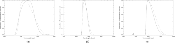
Figure 1. Normalized transmission curves of the RIT filters, solid lines, and the Bessel filters, dashed lines for (a) B filter, (b) V filter, and (c) R filter.
Download figure:
Standard image High-resolution imageWIYN photometric data come from the long program of speckle observations that our group has had there. Photometric results are found in Horch et al. (2004, 2008), and span the time frame of 1997 through 2006. During that interval, two different speckle systems were used, though usually with the same CCD that was used in the Lowell-Tololo observations. More information about the speckle optics used during 1997–2000 can be found in Horch et al. (1999), while from 2001–2006, the RYTSI speckle camera was used.
Although hundreds of binaries were observed at both telescopes, in our initial study, we sought to analyze systems that were well observed and had no major or recent indication of variability. For Lowell-Tololo data, we required at least three independent observations in each of the V and R filters. If the B filter data were also included, three observations were required here as well. For WIYN data, at least two observations were required in each of the three different filters. Because of the larger aperture, these data have greater precision, and so we judged it sufficient to reduce the number of observations in a given filter from three to two. Objects that survived these data cuts were then checked for variability in the General Catalog of Variable Stars (GCVS)9 of Samus' et al. (2006). Most of our objects had no entry in that source, but in four cases, namely, STF 186, GLE 1, AC 4, and BU 178 (HIP 8998, 19917, 32677, and 113184, respectively), we retained the object even though it did have an entry in the GCVS. For these objects, the amplitude and type of the variation was either not given or sufficiently small for our purposes (<0.02 mag). We then examined the data in the Hipparcos Catalog (ESA 1997) and the General Catalog of Photometric Data (GCPD)10 of Mermilliod et al. (1997) and found no evidence of variability significant on the level of this study. All four of these objects were observed at the Lowell-Tololo Telescope. We also checked the reddening and extinction toward each object using the NASA/IPAC dust map available online,11 and found that, as expected due to the relatively small distances to our objects, no correction was needed at the level of our photometry.
Tables 1 and 2 contain the final object lists and input data used in this study for CTIO and WIYN data, respectively. In both cases, the table columns give (1) the Washington Double Star12 (WDS) Catalog number for the system (Mason et al. 2001), which also gives the right ascension and declination of the object in J2000.0 coordinates; (2) the discoverer designation in the WDS for the system; (3) the Hipparcos Catalog number; (4) the filter used; (5) the number of observations of the system in that filter; (6) the Johnson V magnitude of the system; (7) the Johnson B − V color of the system; (8) the parallax of the system, as it appears in the Hipparcos Catalog; and (9) the log of the iron abundance compared to the solar value ([Fe/H]), if known. In most cases, the system V magnitude and B − V color are the average of the Johnson UBV values appearing in the GCPD. The uncertainties given are the standard errors computed from the GCPD data. If no data were available for a particular star in the GCPD, then the values shown in the Hipparcos Catalog were used. Iron abundances are from the Geneva-Copenhagen Catalog (Nordström et al. 2004) unless otherwise stated.
Table 1. Speckle Magnitude Differences and Additional Input Parameters, CTIO Data
| WDS | Discoverer | HIP | Speckle Data | System Parameters | |||||
|---|---|---|---|---|---|---|---|---|---|
| (α, δ J2000.0) | Designation | Filter | No. of Obs. | Δm (mag) | Va (mag) | B − Va (mag) | Parallaxb (mas) | [Fe/H] | |
| 00373−2446 | BU 395 | 2941 | V | 5 | 0.25 ± 0.14 | 5.570 ± 0.005 | 0.722 ± 0.008 | 64.38 ± 1.40 | −0.12 |
| R | 5 | 0.33 ± 0.19 | |||||||
| 01243−0655 | BU 1163 | 6564 | V | 6 | 0.19 ± 0.06 | 5.908 ± 0.004 | 0.404 ± 0.009 | 22.33 ± 0.95 | −0.25 |
| R | 8 | 0.27 ± 0.08 | |||||||
| 01361−2954 | HJ 3447 | 7463 | V | 7 | 1.05 ± 0.06 | 5.685 ± 0.005 | 0.335 ± 0.005 | 16.13 ± 0.97 | +0.01 |
| R | 5 | 1.17 ± 0.02 | |||||||
| 01559 + 0151 | STF 186 | 8998 | B | 3 | 0.76 ± 0.26 | 6.007 ± 0.004 | 0.549 ± 0.005 | 25.71 ± 1.73 | −0.12 |
| V | 8 | 0.56 ± 0.09 | |||||||
| R | 5 | 0.56 ± 0.04 | |||||||
| 03124−4425 | JC 8AB | 14913 | B | 3 | 0.59 ± 0.06 | 5.920 ± 0.010b | 0.440 ± 0.042b | 22.83 ± 0.78 | −0.08 |
| V | 6 | 0.40 ± 0.11 | |||||||
| R | 6 | 0.55 ± 0.08 | |||||||
| 04163−6057 | GLE 1 | 19917 | V | 3 | 0.44 ± 0.38 | 6.360 ± 0.006 | 0.073 ± 0.007 | 08.41 ± 0.53 | ... |
| R | 4 | 0.27 ± 0.21 | |||||||
| 05079 + 0830 | STT 98 | 23879 | V | 6 | 1.18 ± 0.06 | 5.331 ± 0.004 | 0.333 ± 0.004 | 16.84 ± 1.32 | ... |
| R | 5 | 1.04 ± 0.06 | |||||||
| 06490−1509 | AC 4 | 32677 | B | 3 | 1.82 ± 0.06 | 5.390 ± 0.006 | −0.100 ± 0.000 | 05.37 ± 0.86 | ... |
| V | 6 | 1.71 ± 0.08 | |||||||
| R | 4 | 1.71 ± 0.08 | |||||||
| 20375+1436 | BU 151AB | 101769 | V | 8 | 1.20 ± 0.05 | 3.617 ± 0.016 | 0.458 ± 0.019 | 33.49 ± 0.88 | −0.05c |
| R | 7 | 1.14 ± 0.06 | |||||||
| 22300+0426 | STF 2912 | 111062 | V | 6 | 1.50 ± 0.06 | 5.494 ± 0.008 | 0.387 ± 0.006 | 18.93 ± 1.23 | +0.34d |
| R | 4 | 1.35 ± 0.07 | |||||||
| 22552−0459 | BU 178 | 113184 | V | 3 | 1.76 ± 0.10 | 5.715 ± 0.005 | 0.880 ± 0.000 | 11.13 ± 0.95 | +0.09e |
| R | 5 | 1.95 ± 0.10 | |||||||
| 23357−2729 | SEE 492 | 116436 | V | 6 | 1.70 ± 0.04 | 6.650 ± 0.010 | 0.560 ± 0.000 | 25.96 ± 1.11 | −0.10 |
| R | 6 | 1.60 ± 0.04 | |||||||
Notes. aFrom the General Catalog of Photometric Data, or the Hipparcos Catalog. In either case, these measures are on the Johnson system (Johnson 1965). bFrom the Hipparcos Catalog (ESA 1997). cOne of us (B.J.B.) analyzed the spectrum in the ELODIE archive (Moultaka et al. 2004) and obtained this metallicity. dFrom the ELODIE Catalog (Prugniel & Soubiran 2001). eFrom the Catalog of Cayrel de Strobel et al. (2001).
Download table as: ASCIITypeset image
Table 2. Speckle Magnitude Differences and Additional Input Parameters, WIYN Data
| WDS | Discoverer | HIP | Speckle Data | System Parameters | |||||
|---|---|---|---|---|---|---|---|---|---|
| (α, δ J2000.0) | Designation | λ/Δλ (nm) | No. Obs. | Δm (mag) | Va (mag) | B − Va (mag) | Parallaxb (mas) | [Fe/H] | |
| 00495+4404 | HDS 109 | 3857 | 503/40 | 3 | 2.34 ± 0.03 | 7.776 ± 0.031 | 0.594 ± 0.015 | 14.85 ± 1.32 | +0.09 |
| 550/40 | 2 | 2.07 ± 0.24 | |||||||
| 648/41 | 2 | 2.09 ± 0.02 | |||||||
| 698/39 | 2 | 1.96 ± 0.12 | |||||||
| 03496+6318 | CAR 1 | 17891 | 503/40 | 2 | 0.47 ± 0.03 | 5.860 ± 0.020 | 0.187 ± 0.013 | 14.11 ± 0.64 | ... |
| 550/40 | 3 | 0.51 ± 0.03 | |||||||
| 648/41 | 2 | 0.44 ± 0.03 | |||||||
| 698/39 | 7 | 0.53 ± 0.06 | |||||||
| 754/44 | 2 | −0.15 ± 0.54 | |||||||
| 20375+1436 | BU 151AB | 101769 | 550/40 | 8 | 0.97 ± 0.04 | 3.617 ± 0.016 | 0.458 ± 0.019 | 33.49 ± 0.88 | −0.05c |
| 551/10 | 3 | 1.05 ± 0.04 | |||||||
| 648/41 | 4 | 1.13 ± 0.04 | |||||||
| 698/39 | 6 | 1.07 ± 0.02 | |||||||
| 701/12 | 6 | 1.07 ± 0.03 | |||||||
| 754/44 | 6 | 1.12 ± 0.01 | |||||||
| 21145+1000 | STT 535AB | 104858 | 503/40 | 2 | 0.23 ± 0.03 | 4.487 ± 0.008 | 0.495 ± 0.009 | 54.11 ± 0.85 | −0.07 |
| 550/40 | 5 | 0.14 ± 0.06 | |||||||
| 551/10 | 2 | 0.19 ± 0.05d | |||||||
| 648/41 | 5 | 0.28 ± 0.03 | |||||||
| 698/39 | 4 | 0.18 ± 0.06 | |||||||
| 701/12 | 2 | 0.01 ± 0.01 | |||||||
| 754/44 | 3 | −0.04 ± 0.16 | |||||||
| 23375+4922 | COU 2674 | 116578 | 503/40 | 2 | 0.41 ± 0.01 | 8.108 ± 0.031 | 0.503 ± 0.015 | 12.40 ± 1.81 | −0.61 |
| 550/40 | 4 | 0.57 ± 0.04 | |||||||
| 648/41 | 3 | 0.29 ± 0.13 | |||||||
| 23411+4613 | MLR 4 | 116849 | 503/40 | 2 | 0.10 ± 0.06 | 7.060 ± 0.070 | 0.465 ± 0.025 | 14.37 ± 0.84 | −0.05 |
| 550/40 | 4 | 0.30 ± 0.20 | |||||||
| 648/41 | 4 | 0.18 ± 0.10 | |||||||
| 698/39 | 4 | 0.17 ± 0.07 | |||||||
Notes. aFrom the General Catalog of Photometric Data, or the Hipparcos Catalog. In either case, these measures are on the Johnson system (Johnson 1965). bFrom the Hipparcos Catalog (ESA 1997). cOne of us (B.J.B.) analyzed the spectrum in the ELODIE archive (Moultaka et al. 2004) and obtained this metallicity. dThe standard error derived from the two identical measures from the speckle data is zero and has been replaced by a typical expected value here.
Download table as: ASCIITypeset image
2.1. Magnitude and Color Conversions
Since the RIT filters differ from Bessel filters, the Fernie (1983) transformation equations used in Horch et al. (2001) can be improved. In addition, B − V colors and apparent V magnitudes for the binaries are in the standard Johnson filter set (Johnson 1965), which also have slight differences with the Bessel standard filters. Similarly, for WIYN data, a system of transformation equations was needed to convert between the narrow instrumental filters and the Johnson system. The approach here has been a four-step process, which is described in further detail below, and is summarized as follows. (1) The Pickles spectral library (Pickles 1998) was used to develop the transformations to convert the system V magnitudes and B − V colors to instrumental values for the desired speckle filters. (2) The V and B − V values for each system were then converted to instrumental values using these results. (3) These were then used in combination with the speckle magnitude differences to obtain component magnitudes and colors in the speckle filters. (4) Finally, these values were converted back to the Johnson system. The final results in the Johnson system could then be used for isochrone fitting.
The Pickles spectral library (Pickles 1998), containing 131 sample spectra, was used to simulate magnitude measurements, along with the filter and atmospheric transmission curves and the quantum efficiency curve for the CCD. For a filter x, the stellar flux in that filter, fx, is therefore expressed as
where S is the star's flux, A is the atmospheric transmission curve, Fx is the filter transmission curve, and Q is the quantum efficiency of the CCD. In addition, there are losses in the optical system, but these are assumed small enough to ignore in this study. From such a flux, a magnitude is then determined.
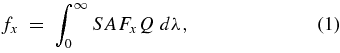
The filter transmission data for the Johnson UBV filters are available at the GCPD Web site. Magnitude values for stars in the Pickles library were calculated in the Johnson filter set and then compared with the values in Schmidt–Kaler (1982). Since these standard literature values assume a quantum efficiency curve that is independent of wavelength, the quantum efficiency curve was omitted from the calculations of colors in the Johnson filter set. This led to a near one-to-one relationship, as seen in Figure 2. For magnitude calculations in both the RIT and WIYN filter sets it was of course necessary to use the quantum efficiency curve, as our observations were taken using the Kodak CCD.

Figure 2. B − V Johnson color magnitudes calculated using the Pickles library and Johnson filter transmission curves, vs. the values found in Schmidt–Kaler. The points were fit with a linear line having a slope of 1.03229, showing our method reproduces the standard color–magnitude values with a small uncertainty.
Download figure:
Standard image High-resolution imageUpon calculating magnitudes for all the sample spectra in each of the essential filters, color–color plots were created. To achieve more accurate relations between colors, and to reduce error, magnitude values were also separated based on luminosity class prior to fitting. A least-squares fit was then performed leading to a polynomial function, in most cases of order three or less, for each luminosity class. This means that, based on the position of the system on the H–R diagram, a preliminary assignment of the luminosity class of the components of each binary was made; in the few cases where the final determination was in conflict with the initial choice, the calculations were redone for that system with the final luminosity class determinations of the first calculation. This then always yielded consistent results in these cases. Also, the Pickles library consists of spectra of single stars, not binaries. By constructing binary spectra of known input magnitude and color difference between the components, we were able to verify that the color–color relations derived based on single stars do not produce errors of more than a few hundredths of a magnitude when used on synthetic binary systems. Since this is in most cases lower than the uncertainties in our input magnitude differences, this source of error can be ignored at this point. However, in the future, when magnitude differences measures are more numerous and the average result in each filter has greater precision, it may be necessary to devise an iterative scheme for ensuring that magnitude and color calibrations do not dominate the errors in the final results.
System colors in the instrumental filter set were used, along with the speckle magnitude differences, to determine magnitudes for the individual stars in all instrumental filters. This is done using the magnitude difference formula
where ma and mb are the magnitudes of the primary and secondary, respectively, and fa and fb are the fluxes for the primary and secondary, respectively. We can then write the same expression for the binary system as a whole and for a zero-magnitude star. Individual magnitudes for the primary and secondary can then be found, through simple calculation. Once all the individual magnitudes have been calculated, colors for the primary and secondary can be trivially derived. Finally, with instrumental parameters in hand for each component of the binary, the V magnitude and B − V color are obtained with the appropriate inverse transformations, obtained again from the Pickles spectral library.
2.2. Isochrone Fitting
Isochrone models were created using Y2 isochrones and the interpolator program from Yale University (Yi et al. 2001, 2003; Kim et al. 2002; Demarque et al. 2004). Solar metallicity isochrones were generally used since, when known, the iron abundance is usually no more than ∼0.1 dex away from solar, and the [Fe/H] determinations are probably uncertain on nearly that same level in most cases. In the cases of three stars, we did elect to interpolate the Y2 isochrones to the metallicity matching the measured iron abundance. These are BU 1163 and COU 2674, which are significantly metal poor, and STF 2912 which is significantly metal rich. Once the metallicity to be used was decided, we created 1800 isochrones for ages of 0.1 to 1.0 Gyr in steps of 0.001 Gyr, and for 1.0 to 9.99 Gyr in steps of 0.01 Gyr. The smaller increments in the younger isochrones were used to provide more precise results for younger systems.
To determine the best fitting, along with upper and lower limit isochrones, we compared our 1800 isochrone models against the primary and secondary positions for a given system. For the purposes of this study, we will refer to the 1σ errors associated with the primary and secondary positions as producing an error "rectangle" in the H–R diagram. The isochrones were first linearly upsampled, by a factor of 100, to fill in any spaces between points, as the models can have large gaps between points in areas where the isochrones are relatively straight, i.e., on the main sequence. Next, the isochrones were checked for points falling within the error rectangles. For isochrones which had points lying within the error rectangles, the shortest overall distance of the primary and secondary to the isochrones were determined. The best-fitting isochrone is simply the one which had the shortest overall distance. The age range for a system was simply determined by finding the youngest and oldest isochrones which passed through both error rectangles.
The best-fitting isochrone was then used to estimate the mass range for both the primary and secondary, by determining the portion of the isochrone which falls within the corresponding 1σ error. From this we estimate the average mass for both primary and secondary, which are only based on the best-fitting isochrone, and combined them to obtain a total mass for the system. We can then compare this against the total dynamical mass from orbital information. The mass fraction,
is also calculated, again using only the best-fitting isochrone, from the average mass of the primary, MA, and secondary, MB.
3. RESULTS
3.1. CTIO Data
Table 3 contains the derived absolute V magnitudes and B − V color magnitudes, in the Johnson filter set, for the components of each system observed at CTIO. Specifically, the columns here give (1) the Discoverer Designation and (2) the Hipparcos Catalog number; (3) the best-fit isochrone age; (4) the age range determined as discussed above; (5) the component identifier for subsequent columns in the table, either A or B; (6) the derived B − V color and (7) absolute V magnitude determination; (8) the luminosity class determination; and (9) the mass derived for the component.
Table 3. Results for CTIO Data
| Discoverer | HIP | Age | Comp. | B − V | Mv | Lum. | Mass | |
|---|---|---|---|---|---|---|---|---|
| Designation | Best Fit | Range | Class | |||||
| BU 395 | 2941 | 9.36 | 0.100–9.99 | A | 0.77 ± 0.14 | 5.31 ± 0.08 | V | 0.90 ± 0.01 |
| B | 0.68 ± 0.19 | 5.55 ± 0.09 | V | 0.87 ± 0.01 | ||||
| BU 1163 | 6564 | 3.38 | 1.55–4.40 | A | 0.46 ± 0.08 | 3.34 ± 0.10 | V | 1.24 ± 0.02 |
| B | 0.36 ± 0.10 | 3.53 ± 0.10 | V | 1.20 ± 0.02 | ||||
| HJ 3447b | 7463 | 1.27 | 0.881–1.56 | A | 0.39 ± 0.10 | 2.10 ± 0.26 | IV | 1.70 ± 0.08 |
| B | 0.22 ± 0.17 | 3.15 ± 0.27 | V | 1.45 ± 0.03 | ||||
| STF 186 | 8998 | 3.62 | 1.12–6.73 | A | 0.54 ± 0.07 | 3.61 ± 0.15 | V | 1.25 ± 0.04 |
| B | 0.55 ± 0.10 | 4.16 ± 0.16 | V | 1.13 ± 0.03 | ||||
| STF 186a | 8998 | 0.696 | 0.100–6.04 | A | 0.44 ± 0.14 | 3.61 ± 0.15 | V | 1.32 ± 0.03 |
| B | 0.76 ± 0.28 | 4.16 ± 0.16 | V | 1.19 ± 0.03 | ||||
| JC 8 AB | 14913 | 1.62 | 1.41–1.67 | A | 0.53 ± 0.10 | 3.31 ± 0.09 | V | 1.34 ± 0.01 |
| B | 0.31 ± 0.15 | 3.71 ± 0.10 | V | 1.27 ± 0.002 | ||||
| JC 8 ABa,b | 14913 | 0.281 | 0.100–3.11 | A | 0.32 ± 0.18 | 3.31 ± 0.17 | V | 1.41 ± 0.05 |
| B | 0.63 ± 0.25 | 3.71 ± 0.19 | V | 1.31 ± 0.05 | ||||
| GLE 1 | 19917 | 0.169 | 0.100–1.07 | A | −0.06 ± 0.34 | 1.55 ± 0.20 | V | 2.14 ± 0.25 |
| B | 0.26 ± 0.44 | 1.98 ± 0.26 | V | 1.90 ± 0.23 | ||||
| STT 98b | 23879 | 1.02 | 0.204–1.49 | A | 0.26 ± 0.11 | 1.80 ± 0.34 | IV | 1.82 ± 0.21 |
| B | 0.53 ± 0.22 | 2.98 ± 0.35 | V | 1.46 ± 0.17 | ||||
| AC 4 | 32677 | 0.195 | 0.100–0.386 | A | −0.10 ± 0.05 | −0.76 ± 0.35 | V | 3.62 ± 0.40 |
| B | −0.08 ± 0.18 | 0.95 ± 0.35 | V | 2.52 ± 0.36 | ||||
| AC 4a | 32677 | 0.151 | 0.100–0.267 | A | −0.13 ± 0.03 | −0.76 ± 0.35 | V | 3.92 ± 0.46 |
| B | 0.06 ± 0.13 | 0.95 ± 0.35 | V | 2.54 ± 0.34 | ||||
| BU 151ABb | 101769 | 1.79 | 1.07–1.96 | A | 0.43 ± 0.14 | 1.58 ± 0.12 | III | 1.75 ± 0.002 |
| B | 0.56 ± 0.25 | 2.79 ± 0.14 | IV | 1.47 ± 0.04 | ||||
| STF 2912 | 111062 | 0.598 | 0.100–0.975 | A | 0.32 ± 0.06 | 2.15 ± 0.14 | IV | 1.82 ± 0.05 |
| B | 0.60 ± 0.12 | 3.65 ± 0.15 | V | 1.36 ± 0.04 | ||||
| BU 178 | 113184 | 2.35 | 1.14–2.88 | A | 0.93 ± 0.10 | 1.20 ± 0.19 | III | 1.62 ± 0.00 |
| B | 0.58 ± 0.19 | 2.96 ± 0.20 | V | 1.42 ± 0.05 | ||||
| SEE 492 | 116436 | 3.42 | 0.100–6.14 | A | 0.54 ± 0.05 | 3.97 ± 0.09 | V | 1.17 ± 0.02 |
| B | 0.70 ± 0.09 | 5.66 ± 0.10 | V | 0.91 ± 0.01 | ||||
Notes. aCalculated using ΔB and a system B − V color magnitude. bThe best-fit isochrone does not simultaneously run through the 1σ error bar for the primary and secondary (but does simultaneously fit the 2σ error bars).
Download table as: ASCIITypeset image
Results were derived for all the systems using speckle ΔV and ΔR magnitudes. For the systems STF 186 (HIP 8998), JC 8AB (HIP 14913), and AC 4 (HIP 32677), a second result was determined using speckle ΔB and ΔV magnitudes. In these cases, observations were not combined to produce a single result in order to examine any differences which arise from observations in the B and R filters, which will be discussed below. While the B − V color values of the components of these systems are generally different by the order of a tenth of a magnitude, the uncertainties are also typically of the same order. This can be traced back to the uncertainty in individual speckle magnitude differences at the small aperture, as well as the number of observations, ⩽8 in every case. Nonetheless, it can be seen in the final columns of Table 3 that the mass values still have very good precision. This is due to the fact that the color of a component gives leverage mainly on the age of the system, whereas the absolute magnitudes derived affect the mass more than the age in the isochrone fitting. The uncertainties in absolute magnitude depend also on distance, but in general translate into modest uncertainties in the masses of the components.
Systems and components were then separately plotted on the H–R diagrams seen in Figure 3. The solid line is the isochrone which best fits the primary and secondary locations, while the dashed lines represents the isochrones that are the upper and lower age limits. Lines marking the zero age main sequence, subgiant sequence, and giant sequence are also drawn.

Figure 3. H–R diagrams for the nine CTIO systems in Table 3 having only V and R measures.
Download figure:
Standard image High-resolution imageFor those systems having two sets of results, the H–R diagrams appear in Figure 4. Differences between using ΔB and ΔR become obvious when comparing these plots. From our results, it is generally the case that the secondary has a redder position in the H–R diagram when the analysis uses the B and V filters as opposed to the V and R filters. Assuming that the components of a system formed at the same time, the results of the R observations would appear to be more realistic. This is particularly noticeable in STF 186 (HIP 8998) and JC 8AB (HIP 14913), which have system locations near the main sequence, and where the components would be expected to have positions more or less on the main sequence, especially for the secondary. One possible explanation for this is that the isoplanatic patch is expected to be smaller as the wavelength of observation decreases, thus affecting the B filter the most. As discussed in Horch et al. (2001), any decorrelation between primary and secondary speckle patterns would lead to an overestimate of the derived magnitude difference. If this effect is most noticeable in the B filter, a redder color could be derived for the secondary star. Since there are only three systems which had sufficient observations in both B and R filters, we cannot draw any definitive conclusions about this; however, the results we have indicate observations taken in the R filter produce position locations which are more consistent with evolutionary calculations.
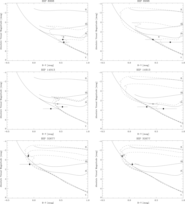
Figure 4. H–R diagrams for three CTIO systems using both V − R (left) and B − V (right) speckle magnitude differences.
Download figure:
Standard image High-resolution image3.2. WIYN Data
For the objects observed at CTIO, typically data in only two filters were available. This meant that usually only one color–color transformation was needed in order to complete the analysis described above. In contrast, the WIYN objects have been observed in at least three, and up to seven, filters. This presents additional work in completing the analysis, though essentially the same method described above was simply used multiple times. For every filter pair that could reasonably be used to generate a color, color–color transformations were created from the Pickles spectral library, and estimates of the component MV and B − V values were obtained. Once all possible estimates were obtained, average values were formed.
In Table 4, we show the results for the component V magnitudes and B − V colors as well as the results from the isochrone fitting for objects observed at the WIYN Telescope. The column headings are exactly the same as in Table 3. In this case, it is possible to see the advantage of the larger aperture, particularly on the derived B − V values for the components. Values for the component masses are likewise relatively precise, with estimated uncertainties under 0.1 solar masses for the primaries in all cases. The H–R diagrams for these systems are shown in Figure 5.

Figure 5. H–R diagrams for the six WIYN systems in Table 4.
Download figure:
Standard image High-resolution imageTable 4. Results for WIYN Data
| Discoverer | HIP | Age | Comp. | B − V | Mv | Lum. | Mass | |
|---|---|---|---|---|---|---|---|---|
| Designation | Best Fit | Range | Class | |||||
| HDS 109 | 3857 | 3.87 | 0.881–5.86 | A | 0.55 ± 0.03 | 3.77 ± 0.44 | V | 1.21 ± 0.09 |
| B | 0.82 ± 0.05 | 6.01 ± 0.44 | V | 0.88 ± 0.03 | ||||
| CAR 1 | 17891 | 0.302 | 0.100–0.468 | A | 0.18 ± 0.02 | 2.14 ± 0.23 | IV | 1.76 ± 0.18 |
| B | 0.20 ± 0.03 | 2.63 ± 0.23 | V | 1.67 ± 0.17 | ||||
| BU 151 AB | 101769 | 1.76 | 1.60–1.94 | A | 0.49 ± 0.02 | 1.60 ± 0.13 | III | 1.760 ± 0.001 |
| B | 0.40 ± 0.04 | 2.63 ± 0.13 | IV | 1.52 ± 0.04 | ||||
| STT 535 | 104858 | 2.34 | 0.76–3.36 | A | 0.50 ± 0.02 | 3.81 ± 0.08 | V | 1.22 ± 0.02 |
| B | 0.52 ± 0.04 | 4.01 ± 0.08 | V | 1.18 ± 0.02 | ||||
| COU 2674 | 116578 | 7.61 | 0.100–9.99 | A | 0.45 ± 0.06 | 4.16 ± 0.73 | V | 0.92 ± 0.07 |
| B | 0.57 ± 0.08 | 4.52 ± 0.73 | V | 0.86 ± 0.04 | ||||
| MLR 4 | 116849 | 2.02 | 0.100–2.57 | A | 0.48 ± 0.03 | 3.51 ± 0.29 | V | 1.27 ± 0.04 |
| B | 0.43 ± 0.05 | 3.65 ± 0.29 | V | 1.29 ± 0.03 | ||||
Download table as: ASCIITypeset image
4. DISCUSSION
Upon surveying the results in Tables 3 and 4, we can first conclude that in most cases the age information is only rudimentary; as most systems are on or near the main sequence, no precise ages can be determined. In a few cases, however, one or both components is evolved. The best example of this is BU 151AB, where from CTIO data the age range matching the H–R diagram positions is 1.07 to 1.96 Gyr with a best-fit value of 1.79 Gyr, and for WIYN data on the same system, it is 1.60 to 1.94 Gyr with a best-fit value of 1.76 Gyr. The excellent agreement between the data sets gives confidence that the photometric conversions are working well. This system is discussed further below.
Tables 5 and 6 provide a comparison between the masses derived here and those available from orbit determinations and other data in the literature. The column headings for both give (1) Hipparcos Catalog number; (2) the mass fraction and (3) total mass calculated from the isochrone fitting, in solar masses; (4) the dynamically determined mass faction, if it exists, and (5) total mass from orbit calculations; and (6) the reference for the orbit calculation. Dynamically determined mass fractions are those appearing in Meyer (2002). In many cases, the orbital parameters are published without uncertainties, meaning that it is not possible to properly account for the contributions of the uncertainties in the semimajor axis and period in the uncertainty of the dynamical mass sum. This is noted in the relevant cases in Column (5) of these tables. The errors shown in these cases are only those due to the uncertainty in the parallax, and while it is true that in most cases the parallax is almost certainly the dominant source of uncertainty in the mass sum, the values listed are still necessarily an underestimate.
Table 5. CTIO Mass Results Compared with Literature Values
| HIP | Photometric Results | Dynamical Results | Orbit Reference | ||
|---|---|---|---|---|---|
| Mass Fraction | Total Mass | Mass Fraction | Mass Sum | ||
| 2941 | 0.49 ± 0.01 | 1.76 ± 0.01 | 0.42 ± 0.02 | 1.77 ± 0.13 | Pourbaix (2000) |
| 6564 | 0.49 ± 0.01 | 2.44 ± 0.03 | 0.52 ± 0.03 | 2.73 ± 0.34a | Söderhjelm (1999) |
| 7463 | 0.46 ± 0.01 | 3.15 ± 0.09 | ... | 3.19 ± 0.72 | Cvetković & Novaković (2006) |
| 8998 (V,R) | 0.48 ± 0.02 | 2.38 ± 0.05 | b | 2.05 ± 0.41a | Brendley & Mason (2007) |
| 8998 (B,V) | 0.48 ± 0.02 | 2.51 ± 0.05 | " | " | " |
| 14913 (V,R) | 0.49 ± 0.002 | 2.61 ± 0.01 | 0.51 ± 0.05 | 2.84 ± 0.29a | Söderhjelm (1999) |
| 14913 (B,V) | 0.48 ± 0.02 | 2.72 ± 0.06 | " | " | " |
| 19917 | 0.47 ± 0.07 | 4.05 ± 0.34 | ... | 5.14 ± 0.97a | Docobo & Ling (2006) |
| 23879 | 0.45 ± 0.07 | 3.28 ± 0.28 | ... | 5.45 ± 1.28a | Scardia et al. (2008) |
| 32677 (V,R) | 0.41 ± 0.07 | 6.15 ± 0.54 | ... | ... | ... |
| 32677 (B,V) | 0.39 ± 0.06 | 6.46 ± 0.57 | " | " | " |
| 101769 | 0.46 ± 0.01 | 3.22 ± 0.04 | 0.45 ± 0.02 | 3.25 ± 0.26a | Alzner (1998) |
| 111062 | 0.43 ± 0.01 | 3.18 ± 0.06 | ... | 3.52 ± 0.69a | Söderhjelm (1999) |
| 113184 | 0.47 ± 0.02 | 3.04 ± 0.05 | ... | 8.67 ± 2.22a | Brendley & Mason (2007) |
| 116436 | 0.44 ± 0.01 | 2.08 ± 0.02 | ... | 1.67 ± 0.21a | Heintz (1984) |
Notes. aThe actual uncertainty is greater than that listed due to the fact that the orbital elements were published without uncertainties. The value given is solely due to parallax. bA value is reported in Meyer (2002); however, it is aphysical, and has not been included.
Download table as: ASCIITypeset image
Table 6. WIYN Mass Results Compared with Literature Values
| HIP | Photometric Results | Dynamical Results | Orbit Reference | ||
|---|---|---|---|---|---|
| Mass Fraction | Total Mass | Mass Fraction | Mass Sum | ||
| 3857 | 0.42 ± 0.03 | 2.08 ± 0.10 | ... | ... | ... |
| 17891 | 0.49 ± 0.06 | 3.43 ± 0.25 | ... | 3.65 ± 0.50a | Zirm & Horch (2002) |
| 101769 | 0.46 ± 0.01 | 3.28 ± 0.04 | 0.45 ± 0.02 | 3.25 ± 0.26a | Alzner (1998) |
| 104858 | 0.49 ± 0.01 | 2.40 ± 0.02 | 0.484 ± 0.004 | 2.42 ± 0.11 | Muterspaugh et al. (2008) |
| 116578 | 0.48 ± 0.03 | 1.78 ± 0.08 | ... | ... | ... |
| 116849 | 0.50 ± 0.02 | 2.56 ± 0.05 | ... | 2.50 ± 0.44 | Hartkopf et al. (1996) |
Note. aThe actual uncertainty is greater than that listed due to the fact that the orbital elements were published without uncertainties. The value given is solely due to parallax.
Download table as: ASCIITypeset image
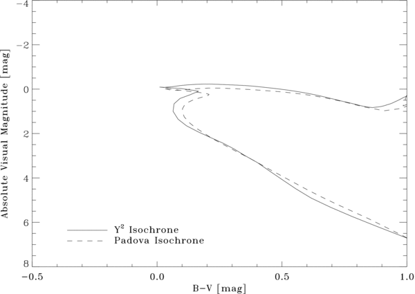
Comparing the mass sums determined photometrically with those determined dynamically, the overall agreement is excellent. The three exceptions to this are for STT 98, BU 178, and SEE 492, which are all discussed in the following subsection. To gauge the degree to which our results depend on the Y2 isochrones, we have compared the result using the Y2 isochrones in some cases with the Padova isochrones of Girardi et al. (2000), also available online.13 Figure 6 shows the result of a typical comparison. In general, we have found little difference between the two sets of isochrones, which is to be expected since many of our systems are main-sequence or just-evolved systems.
Figure 6. Comparison of a Y2 isochrone with a Padova isochrone, both with Solar metallicity and age of 0.598 Gyr.
Download figure:
Standard image High-resolution image
We have also explored the effect of choosing a different metallicity for the isochrone set. This is important especially since some of our systems do not have abundance determinations. We find that the masses derived increase by two to three percent when using metal-rich isochrones with iron abundance +0.34, and decrease approximately seven percent when using metal-poor isochrones with iron abundance −0.25. This indicates that certainly systems with metal abundance in the range −0.15 to +0.15 would suffer only a minor correction from what is derived here using solar values, one which is not significant given our uncertainties at this stage. To be conservative, we have added a 10% uncertainty in quadrature with the uncertainties obtained from the isochrone fitting to mass values to systems for which no iron abundance is available.
4.1. Notes on Specific Systems
Several systems in the data set deserve special mention.
- 1.BU 395 (HIP 2941). Due to the calculation of Pourbaix (2000), we have a very good orbit, listed as Grade 1 in the Sixth Orbit Catalog14 (Hartkopf et al. 2001) and a mass uncertainty of only ∼0.1 M☉. Of the systems observed at CTIO, this is the smallest dynamical mass uncertainty. Our total mass value matches that derived from the Pourbaix orbit almost exactly, although there is a discrepancy in the mass fraction. This will have to be monitored and reevaluated in the coming years as more data become available.
- 2.STT 98 (HIP 23879). The dynamical mass sum of this object is 5.45 M☉ (with an uncertainty of well over 1 M☉, considering that the orbital parameters were published without uncertainties), and the B − V color for the system is 0.334. Given that the components appear to be near the main sequence (with the primary slightly evolved) and that the system has a modest magnitude difference of approximately 1 mag, one would expect spectral types of perhaps F0 and F5. Using data in Schmidt–Kaler, this would yield masses of approximately 1.6 and 1.4 solar masses, that is, a mass sum of approximately 3 solar masses. The orbit is given a grade of 2 in the Sixth Orbit Catalog, but the period is 197 years, so that modern astrometric techniques do not cover the majority of the orbit. We suggest that the mass sum deduced from this orbit may be an overestimate. In our previous work (Horch et al. 2001), we derived preliminary colors and temperatures of the components; the work here is consistent with those earlier results.
- 3.BU 151AB (HIP 101769). As mentioned above, this system consists of two evolved stars, allowing for a relatively precise age determination from both CTIO and WIYN data. The orbit of Alzner (1998) is of excellent quality, easily grade 1 in the Sixth Orbit Catalog, and was produced from high-quality speckle data spanning over a full orbit. This represents one of the most interesting tests of our method, since the uncertainty in the dynamical mass sum is only about three tenths of a solar mass, and the components are evolved. The agreement between the dynamical value and those of both the CTIO and WIYN results is nearly perfect.
- 4.STT 535AB (HIP 104858). This main-sequence system has a very precise orbit determination, published with uncertainties. The uncertainty in the mass sum is only a tenth of a solar mass, making this object the best pure test of our photometrically derived mass values for WIYN data. Our value is well within 1σ of the dynamical value. Our mass fraction also agrees, though we still have an uncertainty of over 10% in this number at present.
- 5.BU178 (HIP 113184). This system has the largest discrepancy between the dynamical mass sum and that derived from the photometric analysis presented here. We find the primary to be a giant, which is consistent with the red system B − V color of ∼0.9, with the secondary still on or near the main sequence. The orbit has a period of 97 years, and the dynamical mass sum is 8.67 ± 2.22 M☉, with the uncertainty being an underestimate due to the lack of error estimates for the orbital elements. The orbit leading to this mass sum is given a grade of 4 in the Sixth Orbit Catalog, but interestingly does include one early interferometric observation of Maggini in 1923 quoted in the 4th Interferometric Catalog. We note that an earlier orbit of Baize (1981), when combined with the Hipparcos parallax, gives a mass sum of nearly 10 M☉, so that at least the accumulation of speckle data since 1981 has decreased the mass somewhat. Nonetheless, we suggest that the dynamical mass value should not be given significant weight at this time.
- 6.SEE 492 (HIP 116436). In this case there is a nearly 2σ discrepancy between the mass sum obtained here and that deduced from the dynamical information. Again, the orbit is listed as grade 4 in the Sixth Orbit Catalog, with a period of 78.5 years. We also note that the most recent observations appear to deviate from the orbit prediction, suggesting that an orbit revision may be needed in the coming years.
5. CONCLUSIONS
Component masses have been estimated for 17 binary star systems using speckle photometry and isochrone fitting. We have shown that our total system masses are consistent with those determined using orbital parameters. Three systems had no prior mass determinations, and the work here has provided component masses for the first time. It has also provided mass fractions in some cases where only a mass sum had previously been determined dynamically. Generally, the results obtained here are of higher precision than the dynamically determined masses. We suggest that this method has promise in the statistical studies of binaries, where it could provide mass information in a relatively short period of time without recourse to orbital data.
We gratefully acknowledge funding from the National Science Foundation, Grants AST 03-07450 and AST 05-04010, which provided support for two of us (J.W.D. and B.J.B.) while graduate students at UMass Dartmouth. We also thank the American Astronomical Society for two small research grants, which funded the observing trips to CTIO. This work made use of the Washington Double Star Catalog maintained at the U.S. Naval Observatory, the SIMBAD database, operated at CDS, Strasbourg, France, and the NASA/IPAC Infrared Science Archive, which is operated by the Jet Propulsion Laboratory, California Institute of Technology, under contract with the National Aeronautics and Space Administration.
Footnotes
- 9
- 10
- 11
- 12
- 13
- 14