


ABSTRACT
We present rotational and radial velocities for a sample of 761 giants selected from the Hipparcos Catalogue to lie within 100 pc of the Sun. Our original goal was to examine stellar rotation in field giants using spectroscopic line broadening to look for evidence of excess rotation that could be attributed to planets that were engulfed as the parent stars expanded. Thus we were obliged to investigate other sources of line broadening, including tidal coupling in close binaries and macroturbulence. For all the binaries in our sample with periods shorter than 20 days the orbits have been circularized, while about half the orbits with periods in the range 20–100 days still show significant eccentricity. All our primaries in orbits shorter than 30 days show line broadening consistent with synchronized rotation, while about half the primaries with periods in the range 30–120 days are synchronized. To study the dependence of rotation on stellar evolution when tidal effects are not important, we used a subsample of single stars and members in wide binaries. We found evidence to suggest that the first dredge-up may play a role in speeding up the rotation of the observable outer layers of giants and that the rotational velocity of horizontal branch stars is larger by a few km s−1 than that of first-ascent giants with similar mass, effective temperature, and radius. Finally, we found three giants that rotate more rapidly than expected. We conjecture that they acquired their excess angular momentum by ingesting planets.
Export citation and abstract BibTeX RIS
1. INTRODUCTION
The discovery of a population of giant planets around solar-type stars in orbits smaller than 1 AU lends some urgency to the question of what happens when a main-sequence star evolves into a giant large enough to engulf such a planet. How much orbital angular momentum from the planet gets converted into excess rotation of the outer layers of the evolving star? Is the effect observable, and how long does it last?
On the theoretical side, the ingestion of giant planets and brown dwarfs by evolving giant stars was studied by Livio (1982), followed by Livio & Soker (1984), Soker et al. (1984), Siess & Livio (1999a, 1999b), and Sandquist et al. (1998, 2002). Various scenarios for the interaction between the companion and the evolving star have been considered. According to Livio & Soker (1984) and Soker et al. (1984), when a giant engulfs a companion smaller than about 20 Jupiter masses, that should lead to its ingestion by the star.
On the observational side, Carney et al. (2003) measured spectral line broadening in a sample of 91 metal-poor red giants and found evidence of excess broadening in a few of the most swollen stars near the tip of the giant branch, and also in some of the post-tip stars on the horizontal branch. They suggested that excess rotation due to ingestion of planets near the tip might be the explanation for the observed excess broadening.
Motivated by this result, that some metal-poor red giants appear to show excess rotation, we undertook a similar survey of a much larger sample of 761 evolved stars drawn from the Hipparcos Catalogue (ESA 1997). Would a sample of solar-metallicity red giants also show evidence for ingested planets? Could the relative frequency of excess rotation between the two samples be used to evaluate the relative roles of core accretion versus disk instability in the formation of giant planets? How about the possibility that the role of planetary migration might depend on metallicity?
As often happens in scientific research, the answers to our naive questions became more elusive as we learned more about the problem. Rotation in an evolving star is not simply the result of conservation of angular momentum applied to an object whose moment of inertia evolves. For single stars, the onset of a stellar wind and magnetic dynamo can provide a strong braking mechanism that carries away rotational angular momentum if the stellar wind is forced to corotate with the star as the wind flows outward. This mechanism is effective at reducing rotation when corotation extends out to several stellar radii. It is thought to be responsible for the dramatic transition from rapid to slow rotation near spectral type F8 on the main sequence (e.g., see Barnes 2000), corresponding to about 1.3  . Lower-mass stars inherit almost no rotation, at least of their observable outer layers, as they evolve away from the main sequence, while higher mass stars inherit projected rotational velocities Vrotsin i that often exceed 100 km s−1 with a Maxwell–Boltzmann distribution (Gray 1989). As these stars cross the so-called granulation boundary on the Hertzsprung–Russell (H–R) diagram (Strassmeier et al. 1998), they develop a convective envelope that gradually deepens, eventually leading to a magnetic dynamo and stellar wind, as evidenced by active coronas. The resulting strong rotational braking is manifested observationally as a sharp transition to slow rotation on the giant branch at spectral type G0 to G3 (Strassmeier et al. 1998; Gray 1989; De Medeiros et al. 1996, 2000, 2003; De Medeiros & Mayor 1999). This strong braking appears to act only until the equatorial rotational velocity falls close to the macroturbulent velocity (Gray 1989). After that stars seem to lose angular momentum slowly (if at all), as they evolve toward the tip of the giant branch during the advanced stages of the hydrogen shell burning phase. Indeed, it has been suggested that the outer layers may actually be spun up if the stellar core is rotating rapidly and a coupling to the observable surface can be established (e.g., see Demarque et al. 2001).
In the case of close binaries, tidal torques can be much stronger than the rotational braking due to magnetic coupling with a stellar wind, and the orbital angular momentum can dominate and control the stellar rotation. Tidal mechanisms tend to align the stellar rotation axes with the orbital axis, to synchronize the rotational periods with the orbital period, and to circularize the orbit, normally with the sequence of events in this order (e.g., see Zahn 1989). Studies of binaries with a giant component include those of Mermilliod & Mayor (1992) and De Medeiros et al. (2002, 2004). Observationally, the transition from eccentric to circular orbits occurs at a period of roughly 150 days for giant binaries in open clusters (e.g., see Mermilliod & Mayor 1992).
Thus, to allow the identification of isolated giants with excess rotation, it was first necessary to identify all the stars where the rotation could be attributed to tidal coupling in a binary. For many of the binaries in our sample, spectroscopic orbits were already available in the literature (e.g., see Pourbaix et al. 2004). For giants that were not known to be binaries, our strategy was to use an initial pair of observations to determine the line broadening. If there was an indication of excess broadening, we then accumulated additional observations over a time span of 1 or 2 years with the goal of identifying all the giants with stellar companions in orbits with periods shorter than a few hundred days, to see if the excess broadening could be attributed to tidal mechanisms. Thus, in 47 cases we accumulated enough observations to allow for orbital solutions using just our own radial velocities, including nine single-lined and four double-lined binaries with no previously published orbits. In addition, we obtained new velocities for 23 binaries with published orbits, so we could update the solutions with modern observations. We also revised four previously published solutions by analyzing the old velocities with modern software. We then used all the stars where tidal mechanisms are negligible to explore how stellar rotation depends on evolutionary stage for giants.
In the end, we were left with only three giants where there is excess rotation that cannot be explained easily and therefore may be due to the ingestion of giant planets.
2. SAMPLE SELECTION
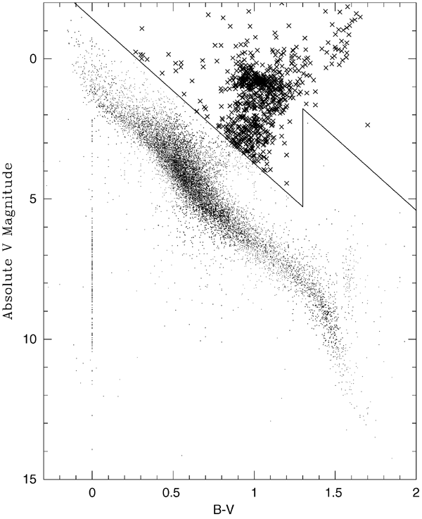
We utilized the Hipparcos Catalogue (ESA 1997) to select a sample of giants with distances within 100 pc. Since the typical accuracy for a Hipparcos parallax is 1 mas, the distances to our targets are accurate to about 10% or better, and the absolute magnitudes to 0.2 mag or better. We limited the sample to the declination range from −20° to +60°, because we wanted to use the CfA Digital Speedometer (Latham 1992) on the 1.5 m Wyeth Reflector at the Oak Ridge Observatory located in the town of Harvard, MA, where the northern limit is set by the fork mount, and the southern limit is set by oak trees. For stars with B − V < 1.3 mag we selected all the giants more than nominally 2.5 mag above the main sequence (absolute V magnitude MV < 1.44 + 5.15(B − V)), for stars with 1.3 ⩽ (B − V) ⩽ 2.5 mag we selected all the giants more than 6 mag above the main sequence (MV < 7.44 + 5.15(B − V)), and for stars redder than (B − V) = 2.5 mag we selected only the giants brighter than apparent magnitude V = 8. The 761 giants selected in this way are plotted with the symbol × on the color versus absolute magnitude diagram in Figure 1, together with the dividing lines defined above. In several cases, the light from these targets is a composite of two or more individual stars, including a giant. Stars meeting the distance and declination criteria but too faint to pass the absolute magnitude selection are plotted as small dots.
Figure 1. Color–magnitude diagram for Hipparcos stars within 100 pc. The giants in our sample are plotted with the symbol ×. Download figure:
Because our sample of giants was selected from the Hipparcos Catalogue to lie within 100 pc, the stars are all quite bright, as shown in Figure 2. More than half the stars are sixth magnitude or brighter, and thus are easy to observe even under mediocre conditions. Indeed, for the brightest stars in the sample we found it necessary to reduce the light entering the spectrograph slit by means of a neutral density filter (or clouds), to avoid pulse pile-up in the photon-counting intensified Reticon detector. Table 1 is a list of our program stars by Hipparcos number, together with the HD, HR, Flamsteed, and Bayer aliases reported by Vizier (Ochsenbein et al. 2000) and the J2000 positions from the 2MASS Catalog (Skrutskie et al. 2006).
Figure 2. Number of program stars as a function of visual magnitude V. Download figure:

Table 1. Program Stars, Aliases, and Positions
| Star | HD | HR | Name | 2MASS RA | 2MASS Dec |
|---|---|---|---|---|---|
| HIP000343... | 225 197 | 9101 | ... | 00 04 19.79 | −16 31 44.3 |
| HIP000443... | 28 | 3 | 33 Psc | 00 05 20.13 | −05 42 27.5 |
| HIP000626... | 290 | ... | ... | 00 07 37.91 | +40 08 52.2 |
| HIP000729... | 448 | 22 | 87 Peg | 00 09 02.43 | +18 12 43.2 |
| HIP000840... | 587 | 29 | ... | 00 10 18.87 | −05 14 54.9 |
Only a portion of this table is shown here to demonstrate its form and content. A machine-readable version of the full table is available.
Download table as: DataTypeset image
3. ROTATIONAL AND RADIAL VELOCITIES
We measured new rotational and radial velocities for all the stars in our sample using the CfA Digital Speedometers (Latham 1992), primarily with the 1.5 m Wyeth Reflector at the Oak Ridge Observatory, but also with nearly identical instruments on the 1.5 m Tillinghast Reflector and on the MMT, both located at the Whipple Observatory atop Mount Hopkins, AZ. These instruments record a single echelle order covering 45 Å centered at 5187 Å using photon-counting intensified Reticon detectors. The spectral resolution of all three CfA Digital Speedometers is nominally 8.5 km s−1, and the typical signal-to-noise ratio (SNR) per resolution element ranged from 15 to 50, depending primarily on the amount of line broadening (rapidly rotating stars were exposed for longer on purpose).
The rotational and radial velocities were determined by cross correlation of the observed spectra against templates drawn from a library of synthetic spectra calculated by Jon Morse for a grid of Kurucz (1992) stellar atmospheres. The library grid has a spacing of 250 K in effective temperature, Teff, 0.5 in log surface gravity, log g, and 0.5 in log metallicity relative to the sun, [Fe/H]. For each star, we selected the template having these three parameters closest to the values that we extracted from information in the literature, as described in the following section. We then ran correlations for the full grid of rotational values, Vrot = 0, 1, 2, 4, 6, 8, 10, 12, 16, 20, 25, 30, 35, 40, 50, 60, 70, 80, 90, 100, 120, 140 km s−1 and calculated the mean value of the peak correlation coefficient at each rotation. Next, we used a quadratic interpolation for the three templates centered on the rotation with the highest correlation coefficient to derive the final line broadening for that choice of template parameters, (Teff, log g, [Fe/H]). Finally, we repeated the process for templates 250 K hotter and 250 K cooler in Teff, and interpolated quadratically to get the final rotation at the Teff derived from photometry.
The final radial velocities for each exposure of a star were calculated using the template rotation that gave the highest correlation coefficient averaged over all the exposures for that star.
The procedures used here to determine rotational velocities are similar to the procedures used by Carney et al. (2003), except that here we used our standard library of synthetic spectra appropriate for solar-metallicity giants, rather than the library with enhanced α-element abundances appropriate for very metal-poor giants. A more important difference is our treatment of macroturbulence in this paper. Our stellar models and synthetic spectra were all calculated assuming a microturbulence of 2 km s−1, which is approximately correct for giants (McWilliam 1990), and a value for macroturbulence of  , which is generally too small for giants. In reality, macroturbulence ranges from about 2 km s−1 for subgiants up to as much as 16 km s−1 for supergiants (e.g., see Figure 4). Thus the rotation of the synthetic template spectrum that gives the best match to an observed spectrum is really a proxy for line broadening, and must be corrected for the larger value of macroturbulence appropriate for the star being observed in order to give an estimate of the actual projected rotational velocity, Vrotsin i, as discussed below.
3.1. Stellar Parameters
To select the optimum template for each star from our library of synthetic spectra, we established the effective temperature, surface gravity, and metallicity from information in the literature and then ran grids of correlations to determine the best rotational velocity (as a proxy for spectral line broadening), as described in the previous section. We derived effective temperatures using published data for three sets of color indexes together with the calibrations from Ramirez & Melendez (2005). In those cases where metallicity values were available from McWilliam (1990) and Valdes et al. (2004), we used the effective temperature calibration corresponding to the published metallicity. For the other stars, we adopted a metallicity of [Fe/H] = −0.15, which is the mean for the stars with published values. The standard deviation from the mean for those stars is σ[Fe/H] = ±0.17, which corresponds to an uncertainty in effective temperature of about σTeff = ±30 K. We also assumed that the role of interstellar reddening was insignificant. For the color indexes, we used the visual broad bands B − V and BT − VT from the Hipparcos Catalogue (ESA 1997); V − J, V − H, and V − K using the infrared JHK magnitudes from 2MASS (Skrutskie et al. 2006); and the DDO narrow bands C(42-45) and C(42-48) from Mermilliod & Nitschelm (1989), when available. Many of the stars in our sample were too bright for the 2MASS instruments, so we only used the 2MASS photometry if the errors were less than 0.017, 0.016, and 0.015 mag in JHK, respectively. The agreement between B − V and DDO temperatures is very good (generally within ±25 K at the 1σ level), while the agreement between these two and the JHK temperatures is not as good (generally about ±60 K at the 1σ level). Table 2 reports the color indexes that we used.
Table 2. Color Indexes
| Star | B − V | BT − VT | V − J | V − H | V − K | C(45 − 48) | C(42 − 45) |
|---|---|---|---|---|---|---|---|
| HIP000343... | 1.099 | 1.295 | ... | ... | ... | 1.213 | 0.932 |
| HIP000443... | 1.040 | 1.220 | ... | ... | ... | 1.190 | 0.912 |
| HIP000626... | 0.947 | 1.102 | 1.707 | 2.165 | 2.245 | ... | ... |
| HIP000729... | 1.045 | 1.227 | ... | ... | ... | ... | ... |
| HIP000840... | 0.978 | 1.142 | ... | ... | ... | 1.163 | 0.870 |
Only a portion of this table is shown here to demonstrate its form and content. A machine-readable version of the full table is available.
Download table as: DataTypeset image
Next, we took advantage of the fact that all our stars had parallaxes measured by Hipparcos to derive bolometric luminosities,  , from the absolute V magnitudes using the bolometric corrections from VandenBerg & Clem (2003). Stellar radii were then obtained using the Stefan–Boltzmann law, L = 4πR2σT4eff. Values for the log of the surface gravity, log g, were taken from Allende Prieto & Lambert (1999) and McWilliam (1990) when available, and were estimated by comparison with theoretical evolutionary tracks (Girardi et al. 2000) for the other stars. Table 3 reports the Hipparcos distance in pc, our Teff values and the standard deviation of the individual sets of values from the mean, σT, plus
  ,
,  , and log g. When the total light of a binary or multiple was resolved into its individual components by the Hipparcos mission, the values reported in Table 3 refer to the giant component. Double-lined binaries are discussed separately in Section 4 and were thereby excluded from Table 3.
Table 3. Physical Parameters of the Program Stars
| Star | d | σd | Teff | σT |  |
 |
log g | Refs | [Fe/H] | Refs |
|---|---|---|---|---|---|---|---|---|---|---|
| HIP000343... | 89 | 7 | 4613 | 5 | 1.65 | 10 | 2.5 | 1 | ... | ... |
| HIP000443... | 39 | 2 | 4699 | 9 | 1.39 | 7 | 2.8 | 1 | −0.31 | 5 |
| HIP000626... | 99 | 7 | 4842 | 24 | 1.30 | 6 | 3.0 | 1 | ... | ... |
| HIP000729... | 90 | 6 | 4710 | 0 | 1.72 | 11 | 2.7 | 1 | −0.01 | 5 |
| HIP000840... | 55 | 3 | 4819 | 10 | 1.15 | 5 | 2.9 | 1 | −0.24 | 5 |
Notes. Entries for Teff, σT,  , and
, and  were left blank for all double-lined binaries and for single-lined binaries with a known composite spectrum. The physical parameters for the giants in these binaries can be found in Tables 14 and 15.
References. (1) Allende Prieto & Lambert (1999), (2) McWilliam (1990), (3) our values, (4) Valdez et al. (2004), and (5) McWilliam (1990).
were left blank for all double-lined binaries and for single-lined binaries with a known composite spectrum. The physical parameters for the giants in these binaries can be found in Tables 14 and 15.
References. (1) Allende Prieto & Lambert (1999), (2) McWilliam (1990), (3) our values, (4) Valdez et al. (2004), and (5) McWilliam (1990).
Only a portion of this table is shown here to demonstrate its form and content. A machine-readable version of the full table is available.
Download table as: DataTypeset image
3.2. Macroturbulence and Stellar Rotation
Macroturbulence and stellar rotation affect the broadening of spectral lines differently, and the two effects can be separated using a Fourier analysis of spectra with very high spectral resolution and signal-to-noise ratio, as shown by Gray (1981). The spectra provided by the CfA Digital Speedometers have neither the spectral resolution nor the SNR to allow such an analysis. Thus we have chosen to determine the total observed line broadening using rotational broadening as a proxy, as described above. Then we correct for the macroturbulence expected for the luminosity and effective temperature of the star involved, based statistically on detailed measurements made by Gray & Nagar (1985), Gray & Toner (1986, 1987), and Gray (1989) using high-quality spectra.
Those authors reported the radial-tangential macroturbulence, ζRT, for each star they observed as a function of the star's spectral type and luminosity class. With the data now available to us, particularly the distances from Hipparcos for the stars they observed, we can render a more quantitative dependence of macroturbulence on the stellar parameters. Our approach is illustrated in Figure 3, where we plot the individual stars from Gray & Nagar (1985), Gray & Toner (1986, 1987), and Gray (1989) on a diagram of  versus log Teff. The values of log Teff were derived using B − V color temperatures, while
  was obtained in the same way as described above for our program stars. Both values are listed in Table 4. The dependence of macroturbulence on these two parameters is reasonably fit by the empirical relation:

Figure 4 displays the actual observed values of ζRT from Gray and collaborators compared to the values calculated with Equation (1). The rms residual of the observed from the fitted values is 1.0 km s−1.
Figure 3. Macroturbulence from Gray and coworkers as a function of Download figure: Figure 4. Gray's measured values of ζRT compared to fitted values from Equation (1). Download figure: and log Teff. The color coding is black for 2 ⩽ ζRT < 5, red for 5 ⩽ ζRT < 7, green for 7 ⩽ ζRT < 9, and blue for ζRT ⩾ 9, all in km s−1.

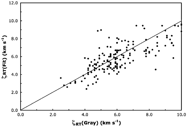
Table 4. Line Broadening Comparison with Measurements of Gray and Coworkers
| CfA | Gray | ||||||||
|---|---|---|---|---|---|---|---|---|---|
| Star | HR |  |
log Teff | Vbr | ζRT | Vrot | Vrot | ζRT | Vbr |
| HIP003031... | 163 | 1.62 | 3.704 | 4.5 | 5.1 | 1.8 | 2.5 | 6.3 | 5.6 |
| HIP003179... | 168 | 2.88 | 3.657 | 10.2 | 7.1 | 8.5 | 4.9 | 6.2 | 6.9 |
| HIP003419... | 188 | 2.13 | 3.681 | 7.3 | 5.6 | 5.8 | 3.0 | 5.9 | 5.6 |
| HIP005951... | 373 | 1.57 | 3.696 | 5.9 | 4.8 | 4.5 | 4.5 | 5.6 | 6.3 |
| HIP008198... | 510 | 2.07 | 3.691 | 5.6 | 5.9 | 3.1 | 2.9 | 4.9 | 4.9 |
| HIP009884... | 617 | 1.91 | 3.653 | 5.2 | 4.0 | 4.2 | 3.1 | 3.9 | 4.4 |
| HIP013531... | 854 | 2.05 | 3.725 | 7.2 | 7.9 | 3.5 | 3.6 | 6.5 | 6.3 |
| HIP015900... | 1030 | 2.11 | 3.705 | 8.0 | 6.8 | 5.9 | 4.8 | 8.0 | 8.0 |
| HIP020205... | 1346 | 1.87 | 3.691 | 6.0 | 5.1 | 4.4 | 2.4 | 5.9 | 5.3 |
| HIP020252... | 1343 | 1.68 | 3.693 | 4.2 | 4.8 | 1.7 | 3.1 | 5.1 | 5.1 |
| HIP020455... | 1373 | 1.83 | 3.688 | 7.0 | 4.9 | 5.8 | 2.5 | 6.2 | 5.5 |
| HIP020885... | 1411 | 1.80 | 3.695 | 5.8 | 5.1 | 4.2 | 3.4 | 4.9 | 5.2 |
| HIP020889... | 1409 | 1.95 | 3.681 | 5.9 | 5.1 | 4.3 | 2.5 | 6.2 | 5.5 |
| HIP031592... | 2429 | 1.06 | 3.671 | 2.4 | 2.8 | 1.0 | 2.7 | 2.7 | 3.4 |
| HIP037826... | 2990 | 1.54 | 3.685 | 4.3 | 4.2 | 2.7 | 2.5 | 4.2 | 4.2 |
| HIP043813... | 3547 | 2.09 | 3.683 | 5.0 | 5.6 | 2.3 | 0.0 | 7.7 | 6.1 |
| HIP046390... | 3748 | 3.10 | 3.605 | 9.5 | 5.3 | 8.5 | 0.0 | 6.5 | 5.2 |
| HIP047908... | 3873 | 2.46 | 3.720 | 11.0 | 9.5 | 8.0 | 4.2 | 7.7 | 7.4 |
| HIP050583... | 4057 | 2.42 | 3.640 | 5.7 | 5.3 | 3.9 | 2.6 | 5.2 | 4.9 |
| HIP069673... | 5340 | 2.21 | 3.636 | 5.3 | 4.5 | 4.0 | 2.4 | 5.2 | 4.8 |
| HIP072105... | 5506 | 2.70 | 3.658 | 12.1 | 6.8 | 10.8 | 6.6 | 9.3 | 9.9 |
| HIP073555... | 5602 | 2.23 | 3.693 | 4.5 | 6.6 | 0.0 | 3.4 | 5.6 | 5.6 |
| HIP074666... | 5681 | 1.70 | 3.690 | 5.1 | 4.8 | 3.5 | 1.1 | 5.7 | 4.7 |
| HIP076219... | 5777 | 1.11 | 3.676 | 5.0 | 3.0 | 4.5 | 3.1 | 2.5 | 3.7 |
| HIP077070... | 5854 | 1.75 | 3.653 | 5.1 | 3.6 | 4.3 | 0.0 | 4.8 | 3.8 |
| HIP078132... | 5940 | 1.55 | 3.660 | 3.3 | 3.3 | 2.0 | 1.1 | 9.3 | 7.5 |
| HIP080816... | 6148 | 2.18 | 3.689 | 5.7 | 6.3 | 2.8 | 3.4 | 6.8 | 6.4 |
| HIP081833... | 6220 | 1.64 | 3.694 | 4.4 | 4.9 | 2.0 | 2.2 | 5.6 | 5.0 |
| HIP086742... | 6603 | 1.80 | 3.652 | 6.1 | 3.6 | 5.4 | 1.6 | 4.0 | 3.6 |
| HIP087933... | 6703 | 1.71 | 3.696 | 4.8 | 5.0 | 2.8 | 3.5 | 5.9 | 5.8 |
| HIP088765... | 6770 | 1.85 | 3.691 | 4.0 | 5.2 | 0.0 | 3.9 | 4.3 | 5.2 |
| HIP089918... | 6866 | 1.84 | 3.700 | 3.7 | 5.6 | 0.0 | 2.6 | 4.4 | 4.4 |
| HIP089962... | 6869 | 1.24 | 3.687 | 3.8 | 3.7 | 2.4 | 2.8 | 2.5 | 3.4 |
| HIP097118... | 7517 | 1.88 | 3.693 | 5.1 | 5.4 | 2.8 | 3.1 | 5.1 | 5.1 |
| HIP100064... | 7754 | 1.59 | 3.691 | 4.5 | 4.5 | 2.7 | 3.2 | 4.6 | 4.9 |
| HIP102488... | 7949 | 1.73 | 3.673 | 3.6 | 4.3 | 1.2 | 3.0 | 4.2 | 4.5 |
| HIP102532... | 7948 | 1.30 | 3.678 | 4.5 | 3.3 | 3.6 | 2.8 | 3.4 | 3.9 |
| HIP103004... | 7995 | 1.73 | 3.710 | 8.1 | 5.7 | 6.7 | 5.9 | 5.9 | 7.5 |
| HIP104459... | 8093 | 1.57 | 3.692 | 3.3 | 4.5 | 0.0 | 2.8 | 4.6 | 4.6 |
| HIP104732... | 8115 | 2.05 | 3.684 | 5.6 | 5.5 | 3.5 | 3.4 | 4.2 | 4.8 |
| HIP105515... | 8167 | 1.87 | 3.700 | 8.4 | 5.7 | 7.0 | 5.6 | 6.2 | 7.5 |
| HIP106481... | 8252 | 1.51 | 3.700 | 5.3 | 4.7 | 3.8 | 2.7 | 5.4 | 5.1 |
| HIP112158... | 8650 | 2.38 | 3.708 | 6.6 | 8.1 | 1.4 | 2.8 | 6.0 | 5.5 |
| HIP112529... | 8670 | 1.70 | 3.692 | 1.8 | 4.8 | 0.0 | 1.3 | 6.5 | 5.3 |
| HIP112748... | 8684 | 1.67 | 3.694 | 5.5 | 4.8 | 4.0 | 2.6 | 4.2 | 4.2 |
| HIP114273... | 8807 | 1.66 | 3.696 | 6.6 | 4.8 | 5.4 | 6.0 | 3.0 | 6.5 |
| HIP114971... | 8852 | 1.68 | 3.698 | 3.2 | 5.0 | 0.0 | 0.0 | 5.5 | 4.4 |
| HIP115919... | 8923 | 1.62 | 3.696 | 5.1 | 4.7 | 3.5 | 3.1 | 5.2 | 5.2 |
| HIP117375... | 9012 | 1.67 | 3.694 | 3.2 | 4.8 | 0.0 | 1.2 | 6.0 | 4.9 |
Notes. To compare the total line broadening determined from the CfA spectra with the results obtained by Gray and coworkers for the same stars, we reconstructed the total line broadening for Gray's observations by adding their published values of Vrot and ζRT in quadratures with the coefficient Cζ in Equation (2) set to 0.63. The values for ζRT used to correct the CfA observations for macroturbulence were derived using Equation (1), and thus match the typical value determined by Gray and coworkers at the same stellar parameters. The CfA values for Vrot were then calculated using Cζ = 0.63 in Equation (2). Column 3: log of the bolometric luminosity of the primary, in solar units  , Column 4: Teff is in kelvin, Columns 5–10: all velocities are in km s−1.
Download table as: ASCIITypeset image
To extract the rotational velocity, Vrotsin i, from our observed line broadening, we subtracted the effects of macroturbulence in quadrature, as was done by Fekel (1997):
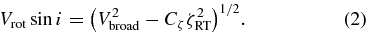
For the coefficient Cζ in this formula, Fekel (1997) adopted the value of 0.5 to take into account the difference in scale between the radial–tangential macroturbulence, ζRT, which is the quantity measured by Gray and collaborators, and the line broadening associated with the Doppler-shift distribution due to macroturbulence. The latter is a more appropriate quantity to subtract in quadrature from the total broadening. Because the macroturbulent velocity dispersion is not expected to be exactly Gaussian (Gray 1992), we chose instead to determine empirically the best value to use for Cζ based on 49 stars in common. We used this procedure to subtract Figure 5. Total line broadening measured at CfA for 49 stars in common with Gray and coworkers and 29 in common with Fekel (1997). Stars in the first group are plotted as filled circles for Download figure: and then add ζRT as calculated using Equation (1). We found that when we used Cζ = 0.63 to reconstruct the total line broadening from the Vrotsin i and ζRT values published by Gray and collaborators, the average difference compared to our line broadening was minimized. We show this comparison for the 49 giants in common with Gray and collaborators in Figure 5, together with 29 stars in common with Fekel (1997). The broadening we observe seems to be systematically larger than Gray's only for stars of very high luminosity,
  , independently of Teff. The rms residuals of our line-broadening values from the 45° line are
  using all 49 stars and
  using the 45 stars with
  . Our reconstruction of the total broadening measured by Fekel (1997) is documented in Table 5.
 and as open circles for
  , while the second group is plotted as filled triangles. The reconstruction of the total line broadening used for Gray and Fekel is documented in Tables 4 and 5, respectively.

Table 5. Line-Broadening Comparison with Measurements of Fekel
| CfA | Fekel | ||||||||
|---|---|---|---|---|---|---|---|---|---|
| Star | HR |  |
log Teff | Vbr | ζRT | Vrot | Vrot | ζRT | Vbr |
| HIP003419... | 188 | 2.13 | 3.681 | 7.3 | 5.6 | 5.8 | 4.0 | 3.0 | 5.0 |
| HIP009884... | 617 | 1.91 | 3.653 | 5.2 | 4.0 | 4.2 | 1.8 | 3.0 | 3.5 |
| HIP019388... | 1283 | 1.75 | 3.669 | 5.6 | 4.1 | 4.6 | 2.2 | 3.0 | 3.7 |
| HIP026366... | 1907 | 1.45 | 3.690 | 3.0 | 4.1 | 0.0 | 0.4 | 3.0 | 3.0 |
| HIP037740... | 2985 | 1.83 | 3.693 | 5.2 | 5.2 | 3.2 | 2.8 | 3.0 | 4.1 |
| HIP037826... | 2990 | 1.54 | 3.685 | 4.3 | 4.2 | 2.7 | 1.7 | 3.0 | 3.4 |
| HIP039311... | 3145 | 2.24 | 3.634 | 5.7 | 4.2 | 4.7 | 2.5 | 3.0 | 3.9 |
| HIP040526... | 3249 | 2.94 | 3.601 | 7.9 | 4.8 | 6.9 | 4.0 | 3.0 | 5.0 |
| HIP048356... | 3903 | 2.16 | 3.697 | 7.1 | 6.5 | 4.9 | 2.9 | 4.0 | 4.9 |
| HIP058948... | 4608 | 1.79 | 3.685 | 2.2 | 4.8 | 0.0 | 2.5 | 3.0 | 3.9 |
| HIP060172... | 4695 | 2.00 | 3.654 | 3.8 | 4.2 | 1.8 | 4.0 | 3.0 | 5.0 |
| HIP063608... | 4932 | 1.82 | 3.696 | 1.9 | 5.3 | 0.0 | 3.2 | 3.0 | 4.4 |
| HIP064022... | 4954 | 2.50 | 3.599 | 6.5 | 3.6 | 5.9 | 3.2 | 3.0 | 4.4 |
| HIP069673... | 5340 | 2.21 | 3.636 | 5.3 | 4.5 | 4.0 | 3.3 | 3.0 | 4.5 |
| HIP070755... | 5409 | 1.10 | 3.743 | 16.0 | 5.1 | 15.5 | 15.7 | 4.0 | 16.2 |
| HIP076534... | 5823 | 1.24 | 3.701 | 2.1 | 4.0 | 0.0 | 0.6 | 2.0 | 2.1 |
| HIP077655... | 5901 | 1.08 | 3.678 | 3.0 | 3.0 | 1.9 | 0.6 | 2.0 | 2.1 |
| HIP078132... | 5940 | 1.55 | 3.660 | 3.3 | 3.3 | 2.0 | 2.2 | 2.0 | 3.0 |
| HIP078159... | 5947 | 2.18 | 3.640 | 4.1 | 4.3 | 2.3 | 1.3 | 3.0 | 3.3 |
| HIP079137... | 6014 | 0.61 | 3.679 | 1.2 | 2.3 | 0.0 | 0.6 | 2.0 | 2.1 |
| HIP080816... | 6148 | 2.18 | 3.689 | 5.7 | 6.3 | 2.8 | 3.0 | 4.0 | 5.0 |
| HIP086742... | 6603 | 1.80 | 3.652 | 6.1 | 3.6 | 5.4 | 2.5 | 3.0 | 3.9 |
| HIP088765... | 6770 | 1.85 | 3.691 | 4.0 | 5.2 | 0.0 | 4.7 | 3.0 | 5.6 |
| HIP089962... | 6869 | 1.24 | 3.687 | 3.8 | 3.7 | 2.4 | 2.6 | 2.0 | 3.3 |
| HIP098110... | 7615 | 1.72 | 3.680 | 4.1 | 4.4 | 2.2 | 1.8 | 3.0 | 3.5 |
| HIP102488... | 7949 | 1.73 | 3.679 | 3.6 | 4.3 | 1.2 | 2.0 | 3.0 | 3.6 |
| HIP102532... | 7948 | 1.30 | 3.678 | 4.5 | 3.3 | 3.6 | 2.9 | 2.0 | 3.5 |
| HIP110882... | 8551 | 1.50 | 3.672 | 3.2 | 3.7 | 1.4 | 1.0 | 3.0 | 3.2 |
| HIP112997... | 8703 | 1.70 | 3.658 | 28.2 | 3.7 | 28.1 | 28.2 | 3.0 | 28.4 |
Notes. The total line broadening for Fekel (1997) was reconstructed using Cζ = 0.5 in Equation (2), Column 3: log of the bolometric luminosity of the primary, in solar units  , Column 4: Teff is in kelvin, Columns 5–10: all velocities are in km s−1.
Download table as: ASCIITypeset image
3.3. Mean Rotational and Radial Velocities and Error Estimates
The results of our velocity measurements for 748 giants with single-lined spectra are summarized in Table 6, where we give the number of observations, Nobs, the time spanned in days, the line broadening 〈Vbr〉, the inferred rotational velocity 〈Vrot〉, the mean radial velocity on the native CfA system, and the uncertainty of the mean value. The uncertainty is either the standard deviation of the mean, i.e. the standard deviation of the individual velocities from the mean, ext, divided by the square root of the number of observations, or the average internal error estimate, int, divided by the square root of Nobs, whichever error is larger. Next, we report e/i, the ratio of the external to internal error, and then χ2 and the probability of getting a χ2 value this big or larger just by chance for a star that is actually constant and errors that are Gaussian (e.g., see Carney et al. 2003). In our experience, stars with χ2 values smaller than 0.001 often prove to be spectroscopic binaries. In the final column, we give the average value of the peak correlation height.
Table 6. Mean Radial Velocities and Error Estimates for Stars with Single-Lined Spectra
| Star | Nobs | Span | 〈Vbr〉 | 〈Vrot〉 | 〈Vrad〉 | ± | ext | int | e/i | χ2 | P(χ2) | 〈ht〉 |
|---|---|---|---|---|---|---|---|---|---|---|---|---|
| HIP000343... | 2 | 283 | 4.1 | 2.8 | 25.98 | 0.22 | 0.23 | 0.31 | 0.73 | 0.53 | 0.465280 | 0.958 |
| HIP000443... | 3 | 93 | 2.1 | 0.0 | −9.45 | 6.68 | 11.57 | 0.35 | 32.64 | 1932.69 | 0.000000 | 0.944 |
| HIP000626... | 9 | 1151 | 4.8 | 3.8 | −26.91 | 1.74 | 5.22 | 0.36 | 14.62 | 1745.30 | 0.000000 | 0.934 |
| HIP000729... | 2 | 237 | 3.3 | 0.6 | −20.23 | 0.21 | 0.20 | 0.30 | 0.68 | 0.47 | 0.493847 | 0.956 |
| HIP000840... | 2 | 285 | 1.5 | 0.0 | 24.49 | 0.41 | 0.58 | 0.35 | 1.68 | 2.84 | 0.092191 | 0.954 |
| HIP000873... | 2 | 244 | 1.4 | 0.0 | 8.39 | 0.23 | 0.21 | 0.33 | 0.65 | 0.43 | 0.510950 | 0.953 |
| HIP001168... | 2 | 100 | 6.6 | 6.0 | −46.26 | 0.57 | 0.80 | 0.57 | 1.40 | 1.97 | 0.160077 | 0.796 |
| HIP001562... | 1 | 0 | 4.5 | 0.4 | 19.35 | 0.30 | 0.00 | 0.30 | 0.00 | 0.00 | 1.000000 | 0.959 |
| HIP001640... | 2 | 15 | 2.9 | 1.9 | 9.68 | 0.22 | 0.04 | 0.32 | 0.12 | 0.02 | 0.900264 | 0.953 |
| HIP001684... | 2 | 20 | 1.2 | 0.0 | −19.97 | 0.23 | 0.33 | 0.33 | 1.00 | 1.01 | 0.315968 | 0.956 |
| HIP002498... | 2 | 16 | 3.6 | 2.7 | −13.30 | 0.23 | 0.30 | 0.33 | 0.91 | 0.83 | 0.362724 | 0.956 |
| HIP002568... | 2 | 293 | 2.2 | 0.0 | −12.07 | 0.20 | 0.02 | 0.28 | 0.09 | 0.01 | 0.930069 | 0.965 |
| HIP003031... | 3 | 407 | 4.5 | 2.0 | −84.43 | 0.20 | 0.26 | 0.35 | 0.76 | 1.12 | 0.571506 | 0.946 |
| HIP003092... | 63 | 4190 | 7.0 | 6.5 | −9.88 | 0.15 | 1.19 | 0.44 | 2.71 | 456.56 | 0.000000 | 0.918 |
Notes. Column 1: star name from Hipparcos, Column 2: number of observations, Column 3: time spanned (days), Column 4: observed spectral line broadening (km s−1), Column 5: derived projected rotational velocity (km s−1), Column 6: mean radial velocity for single-lined spectra (km s−1), Column 7: error in the mean velocity (km s−1), Column 8: external rms residuals in the observed velocities (km s−1), Column 9: internal velocity error estimate (km s−1), Column 10: ratio of external to internal errors, Column 11: χ2, Column 12: χ2 probability, Column 13: mean of the peak correlation height.
Only a portion of this table is shown here to demonstrate its form and content. A machine-readable version of the full table is available.
Download table as: DataTypeset image
In Table 7, we report the individual radial velocities and internal error estimates for the single-lined stars summarized in Table 6. In our sample, 13 of the 761 giants show composite spectra. Tables 8 and 9 report the individual velocities for twelve double-lined and one triple-lined system, respectively. VB and VC are the velocities for the secondary and tertiary components. The single-lined velocities were derived using rvsao (Kurtz & Mink 1998) running inside the IRAF5 environment. The double-lined velocities were derived using TODCOR (Zucker & Mazeh 1994) as implemented at CfA by Guillermo Torres. To derive all three velocities for the triple-lined system HIP 109281, we used the three-dimensional correlation tool TRICOR as implemented at CfA by Guillermo Torres.
Table 7. Single-Lined Radial Velocities
| Star | Tel | Template | HJD | VA | σ(VA) |
|---|---|---|---|---|---|
| HIP000343 | W | t04750g25p00v002 | 245 2962.536 51 | 25.82 | 0.18 |
| HIP000343 | W | t04750g25p00v002 | 245 3245.776 95 | 26.14 | 0.20 |
| HIP000443 | W | t04750g30m05v001 | 245 3284.644 57 | −18.83 | 0.23 |
| HIP000443 | W | t04750g30m05v001 | 245 3339.577 33 | −12.99 | 0.21 |
| HIP000443 | W | t04750g30m05v001 | 245 3378.461 25 | 3.47 | 0.31 |
| HIP000626 | W | t04750g30p00v004 | 245 2978.564 61 | −19.40 | 0.24 |
| HIP000626 | W | t04750g30p00v004 | 245 3247.722 38 | −20.66 | 0.20 |
| HIP000626 | W | t04750g30p00v004 | 245 3320.690 17 | −22.46 | 0.20 |
| HIP000626 | W | t04750g30p00v004 | 245 3400.479 76 | −24.04 | 0.20 |
| HIP000626 | T | t04750g30p00v004 | 245 3718.615 44 | −30.99 | 0.28 |
| HIP000626 | T | t04750g30p00v004 | 245 3749.592 30 | −31.79 | 0.36 |
Notes. Column 1: star name from Hipparcos, Column 2: telescope (W: Wyeth, T: Tillinghast, M: MMT), Column 3: template (see text for code), Column 4: heliocentric Julian date, Column 5: heliocentric radial velocity (km s−1), Column 6: radial velocity error estimate (km s−1).
Only a portion of this table is shown here to demonstrate its form and content. A machine-readable version of the full table is available.
Download table as: DataTypeset image
Table 8. Double-Lined Radial Velocities
| Star | Template A | Template B | HJD | VA | VB |
|---|---|---|---|---|---|
| HIP004463 | t05000g25p00v006 | t05000g25p00v006 | 244 515 96.4723 | 5.94 | −27.25 |
| HIP004463 | t05000g25p00v006 | t05000g25p00v006 | 244 517 15.8360 | 3.33 | −25.85 |
| HIP004463 | t05000g25p00v006 | t05000g25p00v006 | 244 517 54.8656 | −27.29 | 7.62 |
| HIP004463 | t05000g25p00v006 | t05000g25p00v006 | 244 517 76.8265 | −22.47 | 1.12 |
| HIP004463 | t05000g25p00v006 | t05000g25p00v006 | 244 517 96.7528 | −3.43 | −15.99 |
| HIP004463 | t05000g25p00v006 | t05000g25p00v006 | 244 518 57.7099 | −20.64 | −2.21 |
| HIP004463 | t05000g25p00v006 | t05000g25p00v006 | 244 518 78.5848 | −28.62 | 8.05 |
| HIP004463 | t05000g25p00v006 | t05000g25p00v006 | 244 518 99.6052 | −16.18 | −2.83 |
| HIP004463 | t05000g25p00v006 | t05000g25p00v006 | 244 519 27.5150 | 6.49 | −27.15 |
| HIP004463 | t05000g25p00v006 | t05000g25p00v006 | 244 519 48.4851 | 2.03 | −25.51 |
| HIP004463 | t05000g25p00v006 | t05000g25p00v006 | 244 519 65.4669 | −13.51 | −8.35 |
| HIP004463 | t05000g25p00v006 | t05000g25p00v006 | 244 520 80.8165 | −10.47 | −10.50 |
| HIP004463 | t05000g25p00v006 | t05000g25p00v006 | 244 521 14.8611 | −28.23 | 6.31 |
Notes. Column 1: star name from Hipparcos, Column 2: template for primary, Column 3: template for secondary, Column 4: heliocentric Julian date, Column 5: primary heliocentric radial velocity (km s−1), Column 6: secondary heliocentric radial velocity (km s−1).
Only a portion of this table is shown here to demonstrate its form and content. A machine-readable version of the full table is available.
Download table as: DataTypeset image
Table 9. Triple-Lined Radial Velocities
| Star | Template A | Template B | Template C | HJD | VA | VB | VC |
|---|---|---|---|---|---|---|---|
| HIP109281 | t05000g30p00v010 | t05000g30p00v000 | t06000g45p00v000 | 244 529 67.5719 | 28.40 | 12.40 | 2.10 |
| HIP109281 | t05000g30p00v010 | t05000g30p00v000 | t06000g45p00v000 | 244 530 03.4789 | 6.50 | 7.80 | 27.20 |
| HIP109281 | t05000g30p00v010 | t05000g30p00v000 | t06000g45p00v000 | 244 531 83.7636 | 6.40 | 7.30 | 28.60 |
| HIP109281 | t05000g30p00v010 | t05000g30p00v000 | t06000g45p00v000 | 244 532 16.7807 | 26.20 | 11.40 | 4.50 |
| HIP109281 | t05000g30p00v010 | t05000g30p00v000 | t06000g45p00v000 | 244 532 35.7793 | 7.30 | 7.60 | 23.80 |
| HIP109281 | t05000g30p00v010 | t05000g30p00v000 | t06000g45p00v000 | 244 532 42.6450 | 6.80 | 7.20 | 28.30 |
| HIP109281 | t05000g30p00v010 | t05000g30p00v000 | t06000g45p00v000 | 244 532 50.6847 | 7.40 | 7.60 | 26.10 |
| HIP109281 | t05000g30p00v010 | t05000g30p00v000 | t06000g45p00v000 | 244 532 62.7044 | 26.20 | 10.70 | 4.50 |
| HIP109281 | t05000g30p00v010 | t05000g30p00v000 | t06000g45p00v000 | 244 532 78.6020 | 22.80 | 11.80 | 5.20 |
| HIP109281 | t05000g30p00v010 | t05000g30p00v000 | t06000g45p00v000 | 244 532 97.5022 | 6.90 | 7.40 | 26.40 |
| HIP109281 | t05000g30p00v010 | t05000g30p00v000 | t06000g45p00v000 | 244 533 05.5506 | 6.60 | 7.00 | 29.20 |
| HIP109281 | t05000g30p00v010 | t05000g30p00v000 | t06000g45p00v000 | 244 533 13.5270 | 9.10 | 9.30 | 21.60 |
| HIP109281 | t05000g30p00v010 | t05000g30p00v000 | t06000g45p00v000 | 244 533 21.4916 | 25.70 | 11.10 | 4.90 |
| HIP109281 | t05000g30p00v010 | t05000g30p00v000 | t06000g45p00v000 | 244 533 29.4917 | 31.40 | 10.30 | −0.10 |
| HIP109281 | t05000g30p00v010 | t05000g30p00v000 | t06000g45p00v000 | 244 533 48.5866 | 9.90 | 10.00 | 18.90 |
| HIP109281 | t05000g30p00v010 | t05000g30p00v000 | t06000g45p00v000 | 244 533 57.4718 | 7.10 | 7.40 | 28.00 |
| HIP109281 | t05000g30p00v010 | t05000g30p00v000 | t06000g45p00v000 | 244 533 89.4479 | 31.10 | 9.70 | −0.90 |
| HIP109281 | t05000g30p00v010 | t05000g30p00v000 | t06000g45p00v000 | 244 534 75.8803 | 7.20 | 7.50 | 28.50 |
| HIP109281 | t05000g30p00v010 | t05000g30p00v000 | t06000g45p00v000 | 244 536 59.7361 | 5.80 | 6.20 | 29.00 |
| HIP109281 | t05000g30p00v010 | t05000g30p00v000 | t06000g45p00v000 | 244 537 23.5651 | 5.70 | 5.80 | 27.40 |
| HIP109281 | t05000g30p00v010 | t05000g30p00v000 | t06000g45p00v000 | 244 539 22.9362 | 30.20 | 7.20 | 1.80 |
| HIP109281 | t05000g30p00v010 | t05000g30p00v000 | t06000g45p00v000 | 244 539 28.9652 | 25.40 | 8.80 | 1.40 |
| HIP109281 | t05000g30p00v010 | t05000g30p00v000 | t06000g45p00v000 | 244 539 84.8190 | 29.05 | 6.00 | 3.00 |
| HIP109281 | t05000g30p00v010 | t05000g30p00v000 | t06000g45p00v000 | 244 540 72.5369 | 5.60 | 6.10 | 30.50 |
| HIP109281 | t05000g30p00v010 | t05000g30p00v000 | t06000g45p00v000 | 244 542 83.8773 | 25.90 | 9.20 | 1.60 |
Notes. Column 1: star name from Hipparcos, Column 2: template for primary, Column 3: template for secondary, Column 4: template for tertiary, Column 5: heliocentric Julian date, Column 6: primary heliocentric radial velocity (km s−1), Column 7: secondary heliocentric radial velocity (km s−1), Column 8: tertiary heliocentric radial velocity (km s−1).
Download table as: ASCIITypeset image
For each velocity, the synthetic spectrum that was used as the template is designated by a code, where the "t" field specifies the effective temperature, the "g" field gives ten times log g, and the "m" or "p" fields report the metallicity, [Fe/H], also multiplied by 10, with "m" standing for minus and "p" for positive values. The "v" field specifies the rotational velocity. The telescope codes are "W" for the 1.5 m Wyeth Reflector at the Oak Ridge Observatory, "T" for the 1.5 m Tillinghast Reflector at the Whipple Observatory, and "M" for the MMT at the Whipple Observatory.
All of the CfA velocities reported in this paper are on the CfA native system. To put these velocities onto an absolute system defined by minor-planet observations 0.139 km s−1 must be added to the native velocities. No attempt has been made to correct for differences in gravitational redshift between the solar spectrum used to calibrate the CfA velocity zero point and the spectra of the giants studied here.
4. SPECTROSCOPIC BINARIES
Our observational strategy proceeded in two stages. Initially we obtained a well-exposed spectrum suitable for determining the line broadening. In most cases, we followed this up with a second exposure, to check the first observation. If the line broadening from the initial pair of exposures of a star turned out to be less than 5 km s−1, in most cases we did not schedule additional observations. For those stars with more than 5 km s−1 of line broadening, our goal was to obtain enough additional exposures to identify spectroscopic binaries with periods shorter than a few hundred days. Our plan was to accumulate enough spectra to allow orbital solutions for these binaries, but the Oak Ridge Observatory was abruptly shut down before we could achieve that goal. It turns out that this was not a complete disaster, because published orbital solutions were already available for many of the binaries in our sample, and we were able to obtain additional velocities for critical binaries using the CfA Digital Speedometer on the 1.5 m Tillinghast Reflector at the Whipple Observatory.
Our techniques for identifying spectroscopic binaries were similar to those described in Latham et al. (2002) and will not be repeated in detail here. To summarize, we inspected each spectrum and a plot of its correlation function to look for composite spectra. This led to the identification of 12 double-lined binaries, a triple-lined hierarchical triple system (HIP 109281), a double-lined hierarchical triple system (HIP 28734), and a double-lined binary (HIP 61910N) in a quadruple system with a single-lined binary (HIP 61910S). For the stars showing only one set of lines, we calculated the probability that the observed χ2 was due to Gaussian errors for a star with constant velocity, and scrutinized more carefully those cases where the probability was less than 1%. We also reviewed plots of the velocity history and power spectrum for each star.
In Table 10, we report the results of our orbital solutions for 35 single-lined binaries, one of which is the inner binary in the triple system HIP 28734, and in Table 11 the orbital parameters for 12 double-lined binaries, one of which is the inner binary in the triple system HIP 109281. The corresponding velocity curves and individual velocity observations are plotted in Figures 6 and 7.
Download figure: Figure 6. Velocity curves for the CfA single-lined orbital solutions. The individual velocities for primaries are plotted as filled circles. The vertical axes are velocity in km s−1, the horizontal axes are orbital phase. Download figure: Figure 7. Velocity curves for the CfA double-lined orbital solutions. The individual velocities for primaries are plotted as filled circles, the secondaries as open circles. The vertical axes are velocity in km s−1 the horizontal axes are orbital phase. Download figure:
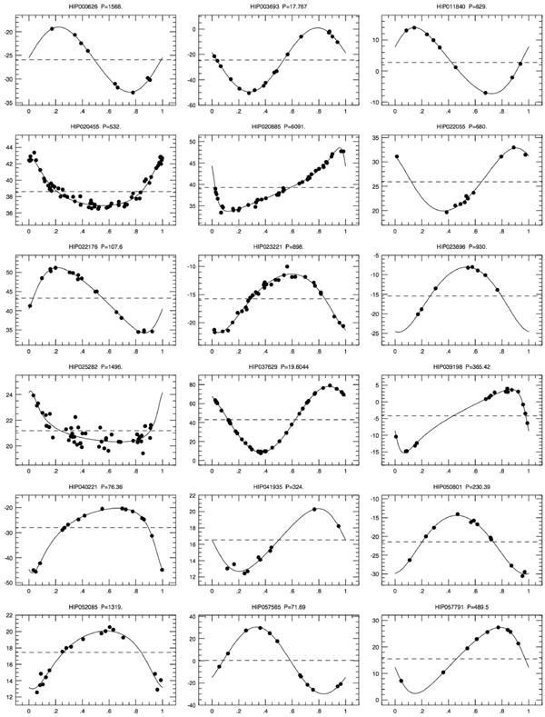
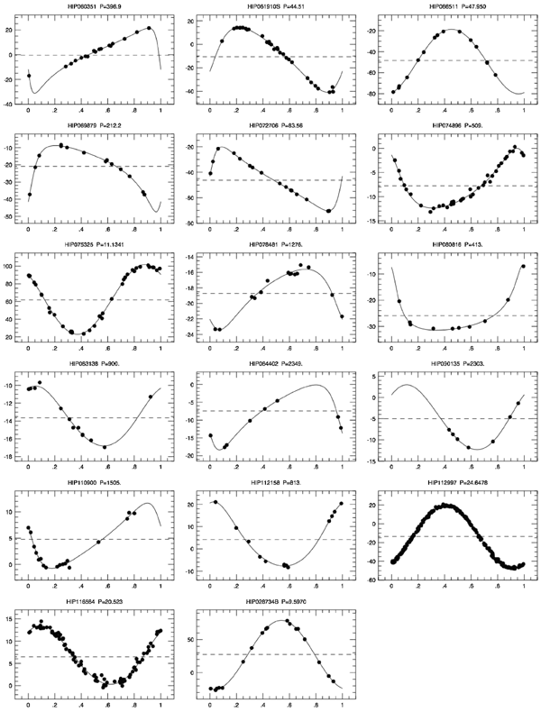
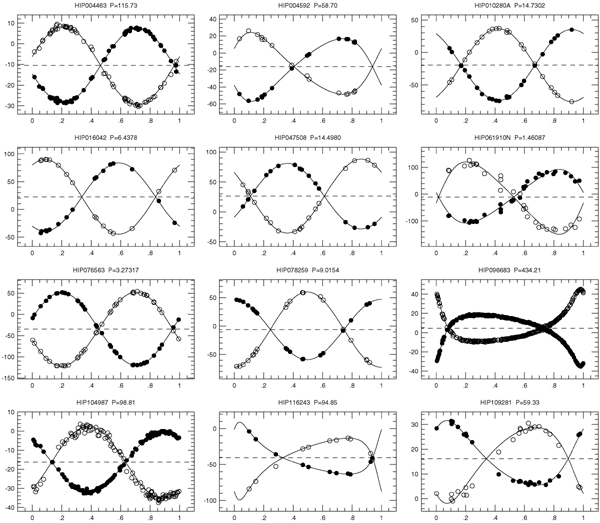
Table 10. CfA Single-Lined Orbital Solutions
| N | Span | |||||||||
|---|---|---|---|---|---|---|---|---|---|---|
| Star | P | γ | K | e | ω | T | aAsin i | f(m) | σ | Cycles |
| HIP000626... | 1568. | −25.92 | 6.87 | 0.06 | 273. | 54276. | 148. | 0.0523 | 9 | 1151.0 |
| ±239. | ±0.46 | ±0.41 | ±0.12 | ±104. | ±377. | ±16. | ±0.0051 | ±0.46 | 0.7 | |
| HIP003693... | 17.7674 | −24.38 | 25.26 | 0.013 | 77. | 53266.2 | 6.17 | 0.0297 | 17 | 382.9 |
| ±0.0048 | ±0.21 | ±0.31 | ±0.011 | ±52. | ±2.6 | ±0.12 | ±0.0017 | ±0.76 | 21.6 | |
| HIP011840... | 629.2 | +2.729 | 10.67 | 0.135 | 294.6 | 53979. | 91.45 | 0.0770 | 9 | 1182.9 |
| ±2.7 | ±0.096 | ±0.13 | ±0.015 | ±6.5 | ±10. | ±0.50 | ±0.0013 | ±0.23 | 1.9 | |
| HIP020455... | 532.0 | +38.598 | 2.904 | 0.415 | 351.1 | 50263.8 | 19.33 | 0.001018 | 61 | 7296.9 |
| ±1.4 | ±0.055 | ±0.076 | ±0.022 | ±4.3 | ±5.3 | ±0.43 | ±0.000067 | ±0.41 | 13.7 | |
| HIP020885... | 6091. | +39.293 | 7.44 | 0.597 | 65.1 | 50999. | 499.8 | 0.1341 | 42 | 5583.0 |
| ±156. | ±0.082 | ±0.14 | ±0.013 | ±2.2 | ±18. | ±9.6 | ±0.0057 | ±0.43 | 0.9 | |
| HIP022055... | 680. | +25.90 | 6.48 | 0.102 | 42. | 53797. | 60.3 | 0.0189 | 11 | 1219.8 |
| ±10. | ±0.51 | ±0.41 | ±0.097 | ±30. | ±52. | ±3.7 | ±0.0033 | ±0.50 | 1.8 | |
| HIP022176... | 107.57 | +43.28 | 8.51 | 0.252 | 254.5 | 49457.5 | 12.19 | 0.00623 | 18 | 1505.9 |
| ±0.12 | ±0.11 | ±0.15 | ±0.019 | ±4.2 | ±1.2 | ±0.19 | ±0.00029 | ±0.45 | 14.0 | |
| HIP023221... | 898.1 | −15.749 | 5.20 | 0.173 | 155.1 | 51240. | 63.2 | 0.01248 | 35 | 4435.1 |
| ±2.7 | ±0.092 | ±0.14 | ±0.025 | ±8.2 | ±21. | ±1.6 | ±0.00095 | ±0.49 | 4.9 | |
| HIP023896... | 930. | −15.45 | 8.31 | 0.114 | 169. | 53622. | 105.5 | 0.0542 | 8 | 1222.9 |
| ±11. | ±0.43 | ±0.85 | ±0.050 | ±18. | ±50. | ±4.1 | ±0.0066 | ±0.21 | 1.3 | |
| HIP025282... | 1496. | +21.18 | 1.98 | 0.60 | 338.7 | 50249. | 33. | 0.00061 | 47 | 8608.5 |
| ±15. | ±0.15 | ±0.74 | ±0.11 | ±8.2 | ±45. | ±10. | ±0.00059 | ±0.55 | 5.8 | |
| HIP037629... | 19.60437 | +43.043 | 34.776 | 0.0143 | 46. | 53507.96 | 9.374 | 0.08540 | 78 | 1252.8 |
| ±0.00053 | ±0.066 | ±0.100 | ±0.0026 | ±13. | ±0.71 | ±0.024 | ±0.00066 | ±0.45 | 63.9 | |
| HIP039198... | 365.42 | −4.23 | 9.56 | 0.515 | 108.1 | 53826.9 | 41.15 | 0.02080 | 17 | 1272.8 |
| ±0.57 | ±0.16 | ±0.17 | ±0.018 | ±3.2 | ±1.3 | ±0.54 | ±0.00082 | ±0.43 | 3.5 | |
| HIP040221... | 76.364 | −27.97 | 12.97 | 0.449 | 153.1 | 53868.89 | 12.17 | 0.01233 | 16 | 1237.8 |
| ±0.030 | ±0.13 | ±0.18 | ±0.013 | ±1.9 | ±0.35 | ±0.18 | ±0.00056 | ±0.50 | 16.2 | |
| HIP041935... | 324. | +16.53 | 3.83 | 0.149 | 90. | 54051. | 16.9 | 0.00183 | 10 | 1190.0 |
| ±10. | ±0.41 | ±0.34 | ±0.096 | ±54. | ±59. | ±1.4 | ±0.00051 | ±0.54 | 3.7 | |
| HIP050801... | 230.39 | −21.44 | 7.82 | 0.103 | 191. | 53764. | 24.64 | 0.0112 | 12 | 1270.9 |
| ±0.52 | ±0.15 | ±0.23 | ±0.027 | ±18. | ±12. | ±0.73 | ±0.0010 | ±0.50 | 5.5 | |
| HIP052085... | 1319. | +17.45 | 3.54 | 0.27 | 163. | 51353. | 62. | 0.0054 | 18 | 6265.0 |
| ±31. | ±0.70 | ±0.43 | ±0.19 | ±18. | ±39. | ±11. | ±0.0031 | ±0.61 | 4.7 | |
| HIP057565... | 71.692 | +0.34 | 30.08 | 0.0039 | 239. | 48837. | 29.66 | 0.2022 | 12 | 1551.9 |
| ±0.012 | ±0.13 | ±0.20 | ±0.0065 | ±122. | ±24. | ±0.16 | ±0.0034 | ±0.42 | 21.6 | |
| HIP057791... | 489.55 | +15.51 | 12.48 | 0.2200 | 102.4 | 53114.4 | 81.97 | 0.0916 | 9 | 1800.1 |
| ±0.97 | ±0.12 | ±0.17 | ±0.0073 | ±3.2 | ±4.2 | ±0.39 | ±0.0013 | ±0.17 | 3.7 | |
| HIP060351... | 396.9 | −0.5 | 26.4 | 0.623 | 105.5 | 53224.9 | 113. | 0.36 | 17 | 2183.1 |
| ±1.4 | ±1.1 | ±4.1 | ±0.051 | ±7.2 | ±4.4 | ±14. | ±0.14 | ±0.62 | 5.5 | |
| HIP061910S... | 44.508 | −10.53 | 27.57 | 0.278 | 249.3 | 53695.02 | 16.21 | 0.0857 | 29 | 1283.8 |
| ±0.010 | ±0.25 | ±0.29 | ±0.012 | ±2.5 | ±0.35 | ±0.33 | ±0.0053 | ±1.01 | 28.8 | |
| HIP066511... | 47.9499 | −48.29 | 30.82 | 0.0369 | 196.2 | 53083.1 | 20.31 | 0.1451 | 16 | 1205.7 |
| ±0.0058 | ±0.12 | ±0.22 | ±0.0067 | ±10.0 | ±1.3 | ±0.12 | ±0.0027 | ±0.44 | 25.1 | |
| HIP069879... | 212.24 | −20.86 | 19.35 | 0.540 | 226.3 | 53859.63 | 47.52 | 0.0949 | 14 | 1207.0 |
| ±0.18 | ±0.17 | ±0.62 | ±0.017 | ±1.9 | ±0.76 | ±0.99 | ±0.0058 | ±0.47 | 5.7 | |
| HIP072706... | 83.556 | −46.326 | 25.16 | 0.5028 | 274.93 | 53300.24 | 24.985 | 0.0890 | 16 | 430.8 |
| ±0.042 | ±0.093 | ±0.19 | ±0.0066 | ±0.80 | ±0.18 | ±0.096 | ±0.0010 | ±0.32 | 5.2 | |
| HIP074896... | 508.7 | −7.743 | 6.19 | 0.327 | 39.0 | 53751.8 | 40.90 | 0.01053 | 38 | 1246.9 |
| ±1.6 | ±0.074 | ±0.12 | ±0.016 | ±3.4 | ±4.0 | ±0.67 | ±0.00051 | ±0.44 | 2.5 | |
| HIP075325... | 11.13413 | +61.90 | 39.52 | 0.021 | 45. | 48278.26 | 6.05 | 0.0711 | 38 | 2578.9 |
| ±0.00036 | ±0.32 | ±0.45 | ±0.012 | ±31. | ±0.96 | ±0.27 | ±0.0095 | ±1.94 | 231.6 | |
| HIP078481... | 1277. | −18.71 | 3.90 | 0.310 | 131. | 54655. | 65.0 | 0.00673 | 15 | 1379.3 |
| ±89. | ±0.25 | ±0.19 | ±0.055 | ±12. | ±104. | ±4.8 | ±0.00094 | ±0.42 | 1.1 | |
| HIP080816... | 413.1 | −25.91 | 12.32 | 0.586 | 19.7 | 53310.9 | 56.7 | 0.0426 | 10 | 1108.1 |
| ±5.1 | ±0.54 | ±0.44 | ±0.036 | ±4.6 | ±9.3 | ±3.0 | ±0.0077 | ±0.53 | 2.7 | |
| HIP083138... | 900. | −13.65 | 3.36 | 0.070 | 338. | 52956. | 41.5 | 0.00352 | 13 | 1323.3 |
| ±14. | ±0.20 | ±0.16 | ±0.068 | ±50. | ±114. | ±1.3 | ±0.00031 | ±0.31 | 1.5 | |
| HIP084402... | 2348.7 | −7.406 | 9.113 | 0.4128 | 119.35 | 53191.1 | 268.08 | 0.13917 | 8 | 2128.2 |
| ±7.5 | ±0.040 | ±0.065 | ±0.0038 | ±0.99 | ±3.7 | ±0.10 | ±0.00019 | ±0.03 | 0.9 | |
| HIP090135... | 2303.33 | −5.017 | 7.636 | 0.0680 | 313.6 | 54441. | 241.2877 | 0.1055055 | 7 | 2160.2 |
| ±0.87 | ±0.019 | ±0.033 | ±0.0011 | ±1.7 | ±11. | ±0.0054 | ±0.0000075 | ±0.00 | 0.9 | |
| HIP110900... | 1505. | +4.79 | 6.22 | 0.370 | 73. | 49171. | 119.6 | 0.0301 | 18 | 4188.6 |
| ±24. | ±0.15 | ±0.49 | ±0.037 | ±14. | ±35. | ±6.8 | ±0.0057 | ±0.49 | 2.8 | |
| HIP112158... | 813. | +4.17 | 14.37 | 0.183 | 344.7 | 52025. | 158.0 | 0.238 | 14 | 1743.3 |
| ±22. | ±0.35 | ±0.37 | ±0.024 | ±8.8 | ±30. | ±4.2 | ±0.018 | ±0.65 | 2.1 | |
| HIP112997... | 24.64784 | −13.594 | 33.376 | 0.0068 | 212. | 50844.3 | 11.312 | 0.0949 | 202 | 2404.6 |
| ±0.00028 | ±0.062 | ±0.087 | ±0.0026 | ±22. | ±1.5 | ±0.051 | ±0.0013 | ±0.87 | 97.6 | |
| HIP116584... | 20.5233 | +6.496 | 6.578 | 0.075 | 322. | 50112.59 | 1.851 | 0.000600 | 82 | 2537.1 |
| ±0.0019 | ±0.068 | ±0.097 | ±0.014 | ±11. | ±0.65 | ±0.033 | ±0.000032 | ±0.60 | 123.6 | |
| HIP028734B... | 9.59697 | +27.59 | 52.15 | 0.014 | 166. | 53240.29 | 6.88 | 0.1410 | 18 | 464.8 |
| ±0.00080 | ±0.29 | ±0.40 | ±0.009 | ±32. | ±0.85 | ±0.13 | ±0.0077 | 1.18 | 48.4 |
Notes. Column 2: period P in days, Column 3: center-of-mass velocity γ in km s−1, Column 4: projected orbital semiamplitude of the primary K in km s−1, Column 5: eccentricity e, Column 6: angle of periastron ω in degrees, Column 7: heliocentric Julian Date −2400,000 for periastron passage T, Column 8: projected semimajor axes of the primary asin i in GM, Column 9: mass function f(m) in  , Column 10: number of velocities and rms velocity residuals in km s−1, Column 11: time spanned by the observations in days and number of orbital cycles covered.
Download table as: ASCIITypeset images: Typeset image Typeset image
Table 11. CfA Double-Lined Orbital Solutions
| P | KA | aAsin i |  |
N | Span | |||||
|---|---|---|---|---|---|---|---|---|---|---|
| Star | q | γ | KB | e | ω | T | aBsin i |  |
σ | Cycles |
| HIP004463... | 115.733 | −10.52 | 17.98 | 0.0032 | 103. | 52662. | 28.61 | 0.3127 | 62 | 2422.3 |
| ±0.023 | ±0.06 | ±0.09 | ±0.0044 | ±75. | ±24. | ±0.15 | ±0.0042 | 0.55 | 20.9 | |
| 0.9446 | ... | 19.03 | ... | ... | ... | 30.29 | 0.2954 | 62 | ... | |
| ±0.0073 | ... | ±0.11 | ... | ... | ... | ±0.18 | ±0.0036 | 0.70 | ... | |
| HIP004592... | 58.700 | −16.14 | 37.04 | 0.2261 | 118.7 | 53590.21 | 29.13 | 1.108 | 16 | 1310.4 |
| ±0.012 | ±0.15 | ±0.21 | ±0.0072 | ±1.4 | ±0.25 | ±0.18 | ±0.031 | 0.55 | 22.3 | |
| 1.016 | ... | 36.47 | ... | ... | ... | 28.67 | 1.125 | 16 | ... | |
| ±0.014 | ... | ±0.43 | ... | ... | ... | ±0.38 | ±0.022 | 1.33 | ... | |
| HIP010280A... | 14.73018 | −19.49 | 54.84 | 0.0035 | 29. | 53353.0 | 11.112 | 1.065 | 22 | 743.0 |
| ±0.00089 | ±0.16 | ±0.36 | ±0.0042 | ±65. | ±2.7 | ±0.079 | ±0.015 | 1.12 | 50.4 | |
| 0.9729 | ... | 56.39 | ... | ... | ... | 11.422 | 1.036 | 22 | ... | |
| ±0.0086 | ... | ±0.29 | ... | ... | ... | ±0.065 | ±0.016 | 0.87 | ... | |
| HIP016042... | 6.43781 | 22.29 | 61.53 | 0.0028 | 149. | 53258.4 | 5.447 | 0.7434 | 17 | 416.9 |
| ±0.00016 | ±0.15 | ±0.57 | ±0.0028 | ±62. | ±1.1 | ±0.056 | ±0.0091 | 1.88 | 64.8 | |
| 0.9153 | ... | 67.22 | ... | ... | ... | 5.951 | 0.680 | 17 | ... | |
| ±0.0097 | ... | ±0.19 | ... | ... | ... | ±0.019 | ±0.014 | 0.52 | ... | |
| HIP047508... | 14.49800 | 26.19 | 54.78 | 0.0022 | 230. | 53132.8 | 10.920 | 1.260 | 18 | 1437.0 |
| ±0.00048 | ±0.17 | ±0.28 | ±0.0048 | ±101. | ±4.2 | ±0.062 | ±0.024 | 0.78 | 99.1 | |
| 0.8869 | ... | 61.76 | ... | ... | ... | 12.31 | 1.118 | 18 | ... | |
| ±0.0091 | ... | ±0.48 | ... | ... | ... | ±0.11 | ±0.016 | 1.38 | ... | |
| HIP061910N... | 1.460866 | −10.8 | 100.3 | 0.211 | 82.1 | 53981.369 | 1.969 | 1.055 | 29 | 1283.8 |
| ±0.000020 | ±1.8 | ±3.1 | ±0.024 | ±6.8 | ±0.026 | ±0.063 | ±0.092 | 11.20 | 878.8 | |
| 0.743 | ... | 134.9 | ... | ... | ... | 2.65 | 0.784 | 29 | ... | |
| ±0.037 | ... | ±5.0 | ... | ... | ... | ±0.10 | ±0.059 | 17.97 | ... | |
| HIP076563... | 3.273167 | −34.35 | 85.67 | 0.0114 | 287.3 | 53309.905 | 3.8556 | 0.8852 | 40 | 1260.5 |
| ±0.000020 | ±0.10 | ±0.18 | ±0.0017 | ±8.3 | ±0.076 | ±0.0087 | ±0.0050 | 0.86 | 385.1 | |
| 0.9815 | ... | 87.28 | ... | ... | ... | 3.928 | 0.8689 | 40 | ... | |
| ±0.0033 | ... | ±0.21 | ... | ... | ... | ±0.010 | ±0.0045 | 0.99 | ... | |
| HIP078259... | 9.01538 | −5.98 | 53.16 | 0.0000 | ... | 53197.2848 | 6.591 | 0.8841 | 21 | 232.6 |
| ±0.00056 | ±0.10 | ±0.13 | Fixed | ... | ±0.0036 | ±0.015 | ±0.0095 | 0.42 | 25.8 | |
| 0.8017 | ... | 66.31 | ... | ... | ... | 8.221 | 0.7088 | 21 | ... | |
| ±0.0048 | ... | ±0.31 | ... | ... | ... | ±0.042 | ±0.0050 | 1.12 | ... | |
| HIP096683... | 434.208 | 4.502 | 26.40 | 0.5557 | 209.41 | 51239.58 | 131.07 | 2.0242 | 291 | 1634.8 |
| ±0.046 | ±0.019 | ±0.05 | ±0.0009 | ±0.13 | ±0.10 | ±0.22 | ±0.0085 | 0.42 | 3.8 | |
| 0.9699 | ... | 27.22 | ... | ... | ... | 135.14 | 1.9633 | 291 | ... | |
| ±0.0024 | ... | ±0.06 | ... | ... | ... | ±0.26 | ±0.0075 | 0.50 | ... | |
| HIP104987... | 98.809 | −16.26 | 15.81 | 0.0069 | 42. | 52717. | 21.48 | 0.2339 | 108 | 2509.3 |
| ±0.014 | ±0.06 | ±0.07 | ±0.0053 | ±40. | ±11. | ±0.10 | ±0.0051 | 0.61 | 25.4 | |
| 0.8348 | ... | 18.93 | ... | ... | ... | 25.72 | 0.1953 | 108 | ... | |
| ±0.0094 | ... | ±0.19 | ... | ... | ... | ±0.26 | ±0.0028 | 1.62 | ... | |
| HIP109281... | 59.331 | 16.22 | 13.03 | 0.237 | 318.0 | 53442.09 | 10.33 | 0.0696 | 25 | 1316.3 |
| ±0.031 | ±0.16 | ±0.25 | ±0.018 | ±4.4 | ±0.61 | ±0.20 | ±0.0053 | 0.79 | 22.2 | |
| 0.849 | ... | 15.34 | ... | ... | ... | 12.16 | 0.0592 | 25 | ... | |
| ±0.032 | ... | ±0.51 | ... | ... | ... | ±0.42 | ±0.0033 | 1.88 | ... | |
| HIP116243... | 94.851 | −40.54 | 36.21 | 0.5169 | 315.82 | 53555.40 | 40.43 | 1.67 | 12 | 1250.5 |
| ±0.013 | ±0.16 | ±0.75 | ±0.0099 | ±0.54 | ±0.13 | ±0.67 | ±0.15 | 0.24 | 13.2 | |
| 0.841 | ... | 43.04 | ... | ... | ... | 48.1 | 1.403 | 12 | ... | |
| ±0.033 | ... | ±1.58 | ... | ... | ... | ±1.9 | ±0.085 | 2.69 | ... |
Notes. Column 2: period P in days, mass ratio q = MmB/MmA, Column 3: center-of-mass velocity γ in km s−1, Column 4: projected orbital velocities of the primary and secondary KA and KB in km s−1, Column 5: eccentricity e, Column 6: angle of periastron ω in degrees, Column 7: heliocentric Julian Date −2400,000 for periastron passage T, Column 8: projected semimajor axes of the primary and secondary aAsin i and aBsin i in GM, Column 9: projected masses of the primary and secondary  and
and  in
in  , Column 10: number of velocities and rms velocity residuals in km s−1 for the primary and secondary, and Column 11: time spanned by the observations in days and number of orbital cycles covered.
Download table as: ASCIITypeset image
Because the nearby giants in our sample are bright, many of them have published orbits, with some of the solutions dating back almost 100 years. For example, the 9th Catalogue of Spectroscopic Binary Orbits (Pourbaix et al. 2004, hereafter SB9) reports single-lined orbital solutions for 60 of the stars in our sample and double-lined solutions for 16 of the stars. Unfortunately, in many cases SB9 does not report errors for the orbital parameters, often because the original publication did not estimate the errors. Therefore, we reviewed the literature for binaries with published orbits, deriving new orbital solutions with error estimates where appropriate, and including new velocities from CfA and other sources when available. The key orbital parameters for these binaries are reported in Tables 12 and 13. The full details for these orbits will be submitted to SB9 and thus they are not documented here.
Table 12. Single-Lined Orbits Using Published Velocities
| Star | P | σP | e | σe | K | σK | Ref. |
|---|---|---|---|---|---|---|---|
| HIP000443... | 72.93 | ... | 0.272 | 0.017 | 16.43 | 0.31 | 4, 00 |
| ... | 72.9404 | 0.0013 | 0.261 | 0.017 | 16.73 | 0.33 | 4, 10, 31, 000 |
| HIP003092... | 21022 | 401 | 0.512 | 0.036 | 4.48 | 0.20 | 21, 22, 23, 24, 10, 000 |
| HIP003675... | 843 | 4 | 0.386 | 0.013 | 5.277 | 0.001 | 62, 00 |
| HIP003693... | 17.769426 | 0.000040 | 0 | Fixed | 25.11 | 0.15 | 5, 00 |
| HIP005951... | 56.824 | 0.011 | 0.00 | Fixed | 7.13 | 0.13 | 6, 00 |
| ... | 56.9 | 0.1 | 0.02 | ... | 7.11 | 0.47 | 66, 00 |
| HIP007143... | 36.588 | 0.024 | 0.203 | 0.031 | 29.97 | 0.88 | 7, 00 |
| ... | 36.598 | 0.034 | 0.189 | 0.051 | 30.0 | 1.5 | 7, 0 |
| ... | 36.355 | 0.001 | 0.111 | 0.035 | 32.03 | 1.11 | 7, 10, 000 |
| HIP007719... | 7581 | 48 | 0.368 | 0.020 | 3.01 | 0.09 | 20, 00 |
| HIP008645... | 1549 | 24 | 0.560 | 0.070 | 3.31 | 0.30 | 25, 0 |
| ... | 1631.6 | 1.5 | 0.648 | 0.038 | 3.83 | 0.23 | 25, 26, 10, 27, 000 |
| HIP008833... | 1672.4 | 1.4 | 0.18 | 0.03 | 4.64 | 0.14 | 28, 00 |
| HIP010366... | 1575.5 | 1.6 | 0.8815 | 0.0010 | 20.37 | 0.09 | 2, 00 |
| HIP011840... | 619.22 | 0.29 | 0.115 | 0.034 | 11.04 | 0.42 | 30, 000 |
| HIP013531... | 1515.81 | 0.05 | 0.729 | 0.004 | 18.97 | 0.20 | 29, 00 |
| HIP015900... | 1654.9 | 2.4 | 0.263 | 0.029 | 4.39 | 0.16 | 15, 00 |
| ... | 1654.1 | 1.2 | 0.271 | 0.036 | 4.41 | 0.18 | 15, 30, 32, 000 |
| HIP020455... | 529.8 | 0.3 | 0.42 | 0.06 | 3.0 | 0.2 | 33, 00 |
| ... | 522.1 | 1.8 | 0.48 | ... | 2.84 | 0.03 | 67, 00 |
| HIP020855... | 5939 | 46 | 0.570 | 0.022 | 7.17 | 0.51 | 63. 00 |
| HIP022176... | 107.503 | 0.023 | 0.210 | 0.017 | 8.51 | 0.15 | 34, 00 |
| HIP023221... | 895.4 | 1.6 | 0.259 | 0.045 | 4.81 | 0.22 | 35, 10, 000 |
| HIP024727... | 434.161 | 0.055 | 0.108 | 0.021 | 14.74 | 0.31 | 10, 26, 30, 32, 000 |
| HIP025282... | 1520 | 17 | 0.55 | 0.12 | 1.54 | 0.23 | 10, 70. 71, 72, 000 |
| HIP028734B... | 9.59659 | 0.00005 | 0.0 | Fixed | 51.7 | 0.3 | 36, 00 |
| HIP028734A... | 4810. | ... | 0.325 | ... | 12. | ... | 37, 00 |
| HIP034608... | 113.346 | 0.006 | 0.400 | 0.014 | 20.75 | 0.38 | 13, 00 |
| HIP037629... | 19.60447 | 0.00007 | 0.0210 | 0.0069 | 34.79 | 0.25 | 38, 00 |
| ... | 19.60415 | 0.00008 | 0.0150 | 0.0038 | 34.58 | 0.13 | 10, 38, 00 |
| HIP039424... | 2437.8 | 2.9 | 0.060 | 0.021 | 5.19 | 0.10 | 39, 00 |
| HIP043109... | 5497.3 | 2.3 | 0.6558 | 0.0018 | 8.05 | 0.14 | 40, 41, 00 |
| HIP045527... | 922 | Fixed | 0.293 | 0.037 | 9.98 | 0.35 | 14, 00 |
| ... | 915.60 | 0.39 | 0.233 | 0.046 | 9.44 | 0.40 | 26, 30, 10, 000 |
| HIP047205... | 2834 | 4 | 0.322 | 0.019 | 6.33 | 0.15 | 42, 00 |
| HIP049841... | 1585.8 | 5.6 | 0.138 | 0.037 | 3.74 | 0.17 | 43 00 |
| ... | 1607.6 | 1.4 | 0.247 | 0.057 | 3.98 | 0.26 | 26, 10, 000 |
| HIP050801... | 230.089 | 0.039 | 0.061 | 0.022 | 7.43 | 0.16 | 15, 00 |
| ... | 230.025 | 0.018 | 0.078 | 0.026 | 7.67 | 0.21 | 15, 000 |
| HIP051233... | 14391 | Fixed | 0.66 | Fixed | 3.18 | 0.34 | 44, 00 |
| ... | 14102 | 315 | 0.754 | 0.051 | 4.45 | 0.48 | 26, 30, 32, 44, 45, 10, 000 |
| HIP052085... | 1345.7 | 5.2 | 0.237 | 0.070 | 4.17 | 0.31 | 10, 000 |
| HIP053240... | 1166 | 7 | 0.375 | 0.035 | 4.40 | 0.21 | 46, 00 |
| HIP057791... | 486.7 | 1.2 | 0.309 | 0.032 | 13.92 | 0.43 | 16, 00 |
| ... | 490.72 | 0.16 | 0.329 | 0.010 | 14.31 | 0.34 | 30, 47, 10, 16, 000 |
| HIP059856... | 1314.3 | 0.4 | 0.426 | 0.016 | 6.54 | 0.13 | 48, 00 |
| HIP060170... | 5792 | 85 | 0.55 | 0.04 | 1.90 | 0.11 | 49, 00 |
| HIP060351... | 396.567 | 0.047 | 0.61 | 0.01 | 25.1 | 0.4 | 17, 00 |
| HIP061724... | 972.4 | 1.4 | 0.590 | 0.007 | 10.46 | 0.13 | 18, 00 |
| HIP061910S... | 44.4137 | 0.0085 | 0.25 | 0.04 | 25.9 | 0.9 | 66,00 |
| ... | 44.4939 | 0.0009 | 0.242 | 0.035 | 25.73 | 0.82 | 66,000 |
| HIP062886... | 2914 | 10 | 0.67 | 0.03 | 5.97 | 0.57 | 64, 00 |
| HIP069879... | 212.085 | 0.002 | 0.574 | 0.005 | 20.14 | 0.17 | 19, 00 |
| HIP075325... | 11.1345 | 0.0005 | 0 | Fixed | 38.6 | 0.4 | 8, 00 |
| HIP076425... | 5324 | 19 | 0.345 | 0.024 | 3.86 | 0.09 | 50, 00 |
| HIP076566... | 14.284 | 0.011 | 0.31 | 0.07 | 9.92 | 0.58 | 11, 00 |
| HIP078259... | 9.01490 | 0.00007 | 0 | Fixed | 53.47 | 0.18 | 9, 00 |
| HIP078481... | 1223.53 | 1.38 | 0.219 | 0.068 | 3.53 | 0.21 | 26, 30, 10, 000 |
| HIP080816... | 410.61 | 0.78 | 0.545 | 0.015 | 12.84 | 0.29 | 51, 0 |
| ... | 411.026 | 0.045 | 0.546 | 0.011 | 13.09 | 0.23 | 51, 23, 24, 32, 10, 000 |
| HIP083138... | 880.47 | 0.68 | 0.119 | 0.071 | 3.36 | 0.21 | 30, 000 |
| HIP083947... | 876.35 | 0.12 | 0.625 | 0.005 | 4.90 | 0.04 | 52, 00 |
| HIP084402... | 2493 | 11 | 0.497 | 0.062 | 8.54 | 1.01 | 10, 68, 69, 000 |
| HIP090135... | 2373.8 | 4.1 | 0.102 | 0.036 | 5.77 | 0.23 | 53, 00 |
| ... | 2380.0 | 2.6 | 0.114 | 0.044 | 5.67 | 0.26 | 53, 000 |
| HIP091751... | 485.3 | 0.3 | 0.209 | 0.011 | 9.68 | 0.12 | 54, 00 |
| HIP092512... | 138.420 | 0.016 | 0.114 | 0.014 | 23.5 | 0.3 | 55, 0 |
| ... | 138.4455 | 0.0043 | 0.129 | 0.019 | 23.17 | 0.49 | 26, 55, 10, 000 |
| HIP092872... | 2994 | 29 | 0.243 | 0.026 | 4.65 | 0.13 | 56, 00 |
| HIP093244... | 1270.6 | 1.1 | 0.272 | 0.026 | 5.17 | 0.13 | 57, 00 |
| HIP094521... | 856 | 39 | 0.66 | ... | 5.99 | 0.40 | 67, 00 |
| HIP095066... | 266.544 | 0.013 | 0.833 | 0.002 | 29.86 | 0.19 | 58, 00 |
| HIP103519... | 635.1 | 0.5 | 0.441 | 0.023 | 6.44 | 0.18 | 59, 00 |
| HIP104732... | 6489 | 31 | 0.22 | 0.03 | 3.31 | 0.12 | 65, 00 |
| HIP112158... | 818.0 | 2.2 | 0.155 | 0.011 | 14.20 | 0.13 | 60, 00 |
| ... | 817.464 | 0.089 | 0.154 | 0.013 | 14.52 | 0.19 | 60, 26, 23, 24, 10, 61, 000 |
| HIP116584... | 20.5212 | 0.0003 | 0.040 | 0.024 | 6.64 | 0.17 | 12, 00 |
Notes. Column 2: period P in days, Column 3: uncertainty in the value of the period σP, Column 4: eccentricity e, Column 5: uncertainty in the value of eccentricity σe, Column 6: projected orbital velocity of the primary K km s−1, Column 7: uncertainty in the value of KA, denoted by σK. Column 8: reference. References. (0) Our solution using the original data, (00) published solution, (000) our solution using the CfA and published data, (1) Pourbaix et al. (2004), (2) De & Udry (1999), (3) Young (1944), (4) Harper (1926), (5) Fekel et al. (1999), (6) Fekel & Eitter (1989), (7) Heard (1940), (8) Fekel et al. (1985), (9) Griffin (1978), (10) Beavers & Eitter (1986), (11) Tokovinin et al. (1998), (12) Walker (1944), (13) Beavers & Salzer (1985), (14) Jones (1928b), (15) Jackson et al. (1957), (16) Ginestet et al. (1985), (17) Abt & Willmarth (1999), (18) Griffin (1981a), (19) Scarfe & Alers (1975), (20) Griffin (1998), (21) Bakos (1976), (22) Lord (1905), (23) Kustner (1908), (24) Lunt (1918), (25) Jones (1928), (26) Campbell & Moore (1928), (27) Tokovinin & Smekhov (2002), (28) Griffin & Herbig (1981), (29) Griffin et al. (1992), (30) Abt (1970), (31) Harper (1935), (32) Harper (1933), (33) Griffin & Gunn (1977), (34) Griffin et al. (1985), (35) Vennes et al. (1998), (36) Griffin & Radford (1976), (37) Ishida (1985), (38) Bopp & Dempsey (1989), (39) Griffin (1982a), (40) Hartkopf et al. (1996). (41) Bakos & Tremko (1987), (42) Griffin (1985), (43) Spencer Jones (1928), (44) Underhill (1963), (45) Abt et al. (1980), (46) Griffin (1980), (47) Snowden & Young (2005), (48) Griffin (1984), (49) Griffin (1991a), (50) Griffin (1991b), (51) Plummer (1908), (52) Griffin (2004), (53) Grobben & Michaelis (1969), (54) Griffin (1982b), (55) Young (1921), (56) Griffin (1981b), (57) Griffin (1982c), (58) Franklin (1952), (59) Radford & Griffin (1975), (60) Crawford (1901), (61) Parsons (1983), (62) Butler (1998), (63) Torres et al. (1997), (64) Griffin et al. (1988), (65) Griffin & Keenan (1992), (66) Sanford & Karr (1942), (67) Setiawan et al. (2004), (68) Andersen (1985), (69) Clark (1989), (70) Andersen et al. (1987), (71) Andersen & Nordström (1983a), (72) Andersen & Nordström (1983b).
Table 13. Published Double-Lined Orbits
| Star | P | σP | e | σe | KA | σKA | KB | σKB | |
|---|---|---|---|---|---|---|---|---|---|
| HIP004463... | 115.7140 | 0.0055 | 0.0081 | 0.0054 | 17.91 | 0.44 | 19.85 | 0.50 | 1 |
| HIP010280A... | 14.732 | ... | 0.04 | ... | 56.5 | ... | 57.0 | ... | 1 |
| HIP014328... | 5329.9 | 1.7 | 0.7856 | 0.0038 | 13.67 | 0.22 | 18.57 | 0.31 | 1 |
| HIP016042... | 6.4378703 | 0.0000069 | 0 | Fixed | 57.86 | 0.17 | 66.98 | 0.04 | 1 |
| ... | 6.437920 | 0.000020 | 0 | Fixed | 58.60 | 0.91 | 66.92 | 0.24 | 1 |
| HIP024608... | 104.0240 | 0.0020 | 0.0015 | 0.0011 | 26.08 | 0.10 | 27.44 | 0.29 | 1 |
| HIP047508... | 14.498080 | 0.000009 | 0.000 | 0.002 | 54.80 | 0.08 | 62.08 | 0.16 | 1 |
| HIP057565... | 71.69060 | 0.00040 | 0 | Fixed | 30.12 | 0.07 | 33.0 | 1.4 | 1 |
| ... | 71.69060 | 0.00058 | 0.0000 | 0.0052 | 29.91 | 0.34 | 32.85 | 0.77 | 1 |
| HIP061910N... | 1.4605 | ... | 0.09 | ... | 88.2 | ... | 100 | ... | 1 |
| HIP065474... | 4.0145 | ... | 0.18 | ... | 120 | ... | 189 | ... | 1 |
| HIP066511... | 47.9578 | 0.0022 | 0.0340 | 0.0030 | 31.07 | 0.10 | 37.2 | 0.6 | 1 |
| HIP076563... | 3.273284 | 0.000073 | 0 | Fixed | 86.35 | 0.49 | 87.97 | 0.51 | 1 |
| HIP084949... | 2018.8 | 0.7 | 0.6720 | 0.0020 | 12.89 | 0.32 | 18.32 | 0.07 | 1 |
| HIP094013... | 28.5903 | 0.0004 | 0.010 | 0.004 | 40.74 | 0.16 | 45.05 | 0.69 | 2 |
| HIP096683... | 434.169 | 0.015 | 0.5420 | 0.0063 | 27.45 | 0.23 | 28.41 | 0.30 | 1 |
| HIP104987... | 98.8215 | 0.0164 | 0.0044 | 0.0072 | 16.06 | 0.34 | 18.37 | 0.72 | 1 |
| HIP112997... | 24.64877 | 0.00003 | 0 | Fixed | 34.29 | 0.04 | 62.31 | 0.06 | 3 |
Notes. Column 2: period P in days, Column 3: uncertainty in the value of the period σP, Column 4: eccentricity e, Column 5: uncertainty in the value of eccentricity σe, Column 6: projected orbital velocity of the primary KA km s−1, Column 7: uncertainty in the value of KA, denoted by σKA Column 8: projected orbital velocity of the secondary KB in km s−1, Column 9: uncertainty in the value of KB, denoted by σKB. References. (1) Pourbaix et al. (2004), (2) De & Udry (1999), and (3) Marsden et al. (2005).
Download table as: ASCIITypeset image
4.1. Tidal Circularization
Close binaries are subject to tidal interactions that tend to synchronize the rotational periods with the orbital periods and to circularize the orbits, normally with the sequence of events in this order (Zahn 1977, 1989, 1992). For most binaries in the solar neighborhood with orbital periods longer than about 10 days, the stellar radii are too small for tidal circularization to be important as long as both stars are on the main sequence (e.g., see Duquennoy & Mayor 1991; Mathieu et al. 1992; Latham et al. 2002). When the more massive primary star begins to evolve away from the main sequence, its radius swells, the convective envelope grows, and tidal torques can become important. The time scale for tidal circularization can be very short compared to the evolutionary time scale of the primary, because the tidal torques depend very strongly on the ratio of stellar radius to the separation of the two stars.
The location of our 79 giants in 75 binary systems with orbital solutions on a log Teff versus Figure 8. Distribution in Download figure: diagram is shown in Figure 8, together with Girardi et al. (2000) representative evolutionary tracks for stars with mass 1.0, 1.4, 1.8, 2.2, 3.0
  and metallicity [Fe/H] = −0.2, which is close to the average value in the solar neighborhood (e.g., see McWilliam 1990; Nordström et al. 2004). In the region of the diagram where the tracks for different masses and evolutionary stages overlap, one cannot distinguish between stars that are on the first ascent up the giant branch (FA) and stars that have already passed the tip of the giant branch (PT) and are now either on the horizontal branch (HB) or the asymptotic giant branch (AGB). The determination of mass and age for these stars is therefore ambiguous.
 versus log Teff for 67 giants in single-lined binaries and 12 giants in eight double-lined binaries with orbital solutions. The dashed lines represent the Girardi et al. (2000) evolutionary tracks for masses
  and metallicity [Fe/H] =−0.2. Black stands for single-lined binaries, red for the giant component of double-lined binaries. Filled circles represent stars unambiguously on their first ascent to the tip of the red giant branch, while open circles represent stars that could be either in their first ascent to the red giant tip or already in the HB/AGB evolutionary phase. The bar links the primary and the secondary of HIP 78259. HIP 50801, a star unambiguously in its AGB phase, is also represented by an open circle.

Figures 9 and 10 display the orbital eccentricity and the measured Vrotsin i as a function of the orbital period P for the binaries in our sample. In both figures, the filled circles are used for stars unambiguously in the first ascent, while open circles are used for systems of ambiguous evolutionary stage, as defined in Figure 8. For all the binaries in our sample with periods shorter than 20 days the orbits have been circularized, while about half the orbits with periods in the range 20–100 days still show significant eccentricity. All of the eccentric orbits with periods shorter than 120 days are unambiguously on the first ascent. This is not surprising, because the process of circularization strongly depends on the stellar radius, and the average radius of the stars in the first ascent subsample is smaller than that of the ambiguous subsample. All binaries with a period shorter than about 30 days and about half of those with periods between 30 and 120 days appear to be synchronized.
Figure 9. Eccentricity versus orbital period for 75 binary systems. Filled circles stand for the subgroup unambiguously on the first ascent to the red giant tip. Open circles stand for stars whose evolutionary status is ambiguous. Binaries in the latter subgroup may be either on their first ascent or already in their HB or AGB evolutionary phase. HIP 50801, a star unambiguously in its AGB phase, is also represented by an open circle. Download figure: Figure 10. Vrotsin i versus orbital period P for 79 giants in 75 binary systems. Filled circles stand for the subgroup unambiguously on the first ascent to the red giant tip. Open circles stand for stars whose evolutionary status is ambiguous. Binaries in the latter subgroup may either be on their first ascent or already in their HB or AGB evolutionary phase. HIP 50801, a star unambiguously in its AGB phase, is also represented by an open circle. Download figure:
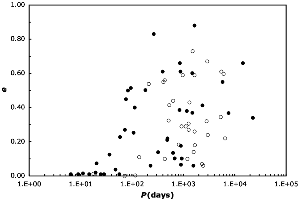
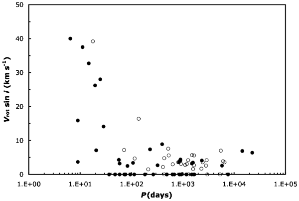
In Tables 14 and 15, we display the main physical parameters that we infer for these stars. These parameters include log Teff,  ,
,  , and mass. For the stellar mass, the tables include values corresponding to tracks on the first ascent
  and post-tip
  : both values are reported for stars whose evolutionary stage is ambiguous. In determining stellar masses, we took into account metallicity when possible and otherwise used the sample average. In the case of double-lined binaries observed at CfA, we adopted the effective temperature for the secondary that gave the best correlations in our TODCOR (Zucker & Mazeh 1994) analysis of our observed spectra. We then subtracted the contribution of the secondary from the total observed V and B − V (using the light ratio from our TODCOR analysis, also reported in Table 15, and adopting a B − V for the secondary corresponding to its effective temperature) in order to derive an effective temperature and luminosity for the primary from the photometry, and then for the secondary. For FA giants, where the evolutionary stage is unambiguous, the evolutionary tracks then allow an estimate of the mass ratio. In all cases, this mass ratio was consistent with the mass ratio from the orbital solution.
Table 14. Single-Lined Primaries with Giants: Physical Parameters
| Star | Vrot |  |
log Teff |  |
 |
 |
Note |
|---|---|---|---|---|---|---|---|
| HIP000443 | 0.0 | 1.38 | 3.669 | 7.4 | 1.3 | ... | ... |
| HIP000626 | 3.8 | 1.29 | 3.684 | 6.3 | 1.5 | ... | ... |
| HIP003092 | 6.5 | 1.87 | 3.635 | 15.7 | 1.2 | ... | ... |
| HIP003675 | 3.6 | 1.60 | 3.682 | 9.1 | 1.9 | ... | ... |
| HIP003693 | 39.3 | 1.92 | 3.662 | 14.4 | 1.8 | 1.4 | ... |
| HIP005951 | 4.5 | 1.56 | 3.695 | 7.9 | 2.0 | ... | ... |
| HIP007143 | 0.0 | 0.80 | 3.687 | 3.5 | 1.2 | ... | ... |
| HIP007719 | 0.0 | 1.66 | 3.700 | 8.9 | 2.4 | ... | ... |
| HIP008645 | 3.2 | 2.38 | 3.661 | 24.5 | 3.0 | 3.0 | ... |
| HIP008833 | 0.0 | 1.65 | 3.694 | 9.1 | 2.5 | 2.2 | ... |
| HIP010366 | 0.0 | 1.41 | 3.684 | 7.0 | 1.5 | ... | ... |
| HIP011840 | 0.0 | 1.52 | 3.665 | 8.9 | 1.3 | ... | ... |
| HIP013531 | 3.5 | 2.03 | 3.677 | 15.2 | 2.6 | 2.2 | 1 |
| HIP015900 | 5.9 | 2.10 | 3.704 | 14.6 | 3.1 | 3.0 | ... |
| HIP020455 | 5.8 | 1.82 | 3.688 | 11.6 | 2.5 | 2.2 | ... |
| HIP020885 | 4.2 | 1.80 | 3.695 | 11.0 | 2.7 | 2.5 | ... |
| HIP022055 | 0.0 | 0.92 | 3.719 | 3.5 | 1.6 | ... | ... |
| HIP022176 | 3.7 | 1.66 | 3.643 | 11.7 | 1.0 | ... | ... |
| HIP023221 | 4.3 | 1.20 | 3.718 | 4.8 | 1.9 | ... | ... |
| HIP023896 | 0.0 | 1.08 | 3.679 | 5.0 | 1.2 | ... | ... |
| HIP024727 | 0.0 | 2.05 | 3.631 | 18.8 | 1.1 | ... | ... |
| HIP025282 | 1.1 | 1.40 | 3.685 | 7.0 | 1.7 | ... | ... |
| HIP034608 | 0.0 | 0.71 | 3.694 | 3.1 | 1.2 | ... | ... |
| HIP037629 | 26.2 | 1.53 | 3.659 | 9.3 | 1.4 | ... | ... |
| HIP039198 | 0.0 | 0.98 | 3.709 | 3.9 | 1.7 | ... | ... |
| HIP039424 | 3.9 | 1.90 | 3.660 | 14.5 | 2.2 | 1.4 | ... |
| HIP040221 | 0.0 | 0.71 | 3.692 | 3.1 | 1.1 | ... | ... |
| HIP041935 | 3.1 | 1.34 | 3.659 | 7.5 | 1.0 | ... | ... |
| HIP043109 | 7.2 | 1.68 | 3.683 | 9.9 | 2.0 | 1.7 | 1 |
| HIP045527 | 3.4 | 1.88 | 3.649 | 14.5 | 1.4 | 1.0 | ... |
| HIP047205 | 3.0 | 1.71 | 3.672 | 10.8 | 1.7 | 1.3 | ... |
| HIP049841 | 2.1 | 1.66 | 3.682 | 10.0 | 2.2 | 1.9 | ... |
| HIP050801 | 7.5 | 3.06 | 3.590 | 74.7 | ... | 2.2 | ... |
| HIP051233 | 7.0 | 1.56 | 3.699 | 8.0 | 2.2 | 2.2 | ... |
| HIP052085 | 3.5 | 1.66 | 3.695 | 9.1 | 2.2 | 2.2 | ... |
| HIP053240 | 0.5 | 1.31 | 3.696 | 6.1 | 1.8 | ... | ... |
| HIP057791 | 1.3 | 1.58 | 3.672 | 9.3 | 1.5 | 1.0 | ... |
| HIP059856 | 0.6 | 2.04 | 3.652 | 17.1 | 1.6 | 1.2 | ... |
| HIP060170 | 2.9 | 1.23 | 3.660 | 6.5 | 1.0 | ... | ... |
| HIP060351 | 9.0 | 1.59 | 3.719 | 7.5 | 2.5 | ... | 1 |
| HIP061724 | 1.5 | 1.68 | 3.684 | 9.9 | 2.0 | 1.8 | ... |
| HIP062886 | 4.2 | 1.97 | 3.700 | 13.0 | 3.0 | 3.0 | ... |
| HIP066511 | 0.0 | 1.05 | 3.684 | 4.8 | 1.3 | ... | ... |
| HIP069879 | 2.1 | 1.79 | 3.670 | 11.9 | 1.8 | 1.4 | ... |
| HIP072706 | 2.9 | 0.84 | 3.673 | 3.9 | 1.0 | ... | ... |
| HIP074896 | 7.7 | 1.62 | 3.687 | 9.0 | 2.2 | 2.2 | ... |
| HIP075325 | 37.6 | 1.08 | 3.662 | 5.4 | 1.0 | ... | ... |
| HIP076425 | 1.4 | 1.57 | 3.690 | 8.4 | 2.2 | 2.2 | ... |
| HIP078481 | 1.2 | 1.91 | 3.679 | 13.0 | 2.3 | 1.9 | ... |
| HIP080816 | 2.8 | 2.17 | 3.688 | 16.9 | 3.0 | 3.0 | ... |
| HIP083138 | 4.6 | 1.60 | 3.652 | 10.4 | 1.2 | ... | ... |
| HIP083947 | 4.3 | 2.01 | 3.634 | 18.0 | 1.2 | ... | ... |
| HIP084402 | 3.1 | 1.62 | 3.663 | 10.1 | 1.4 | 1.0 | ... |
| HIP090135 | 2.2 | 1.65 | 3.688 | 9.3 | 2.2 | 1.8 | ... |
| HIP091751 | 0.0 | 1.31 | 3.677 | 6.6 | 1.4 | ... | ... |
| HIP092512 | 16.5 | 2.24 | 3.643 | 21.8 | 1.8 | 1.6 | ... |
| HIP092872 | 0.0 | 1.70 | 3.671 | 10.6 | 1.8 | 1.0 | ... |
| HIP093244 | 4.4 | 1.78 | 3.671 | 11.9 | 2.0 | 1.4 | ... |
| HIP094013 | 14.1 | 1.40 | 3.668 | 7.7 | 1.2 | ... | ... |
| HIP094521 | 0.0 | 1.05 | 3.685 | 4.8 | 1.4 | ... | ... |
| HIP095066 | 1.2 | 1.32 | 3.691 | 6.3 | 1.8 | ... | ... |
| HIP103519 | 3.3 | 1.59 | 3.686 | 8.9 | 2.2 | ... | ... |
| HIP104732 | 3.6 | 2.05 | 3.685 | 15.2 | 3.0 | 3.0 | ... |
| HIP110900 | 3.4 | 0.73 | 3.691 | 3.2 | 1.2 | ... | ... |
| HIP112158 | 4.0 | 2.38 | 3.682 | 22.2 | 3.5 | 3.5 | 1 |
| HIP112997 | 28.1 | 1.70 | 3.660 | 11.5 | 1.4 | ... | ... |
| HIP116584 | 7.3 | 1.29 | 3.676 | 6.3 | 1.3 | ... | ... |
Notes. Column 2: projected rotational velocity Vrotsin i for the primary, km s−1, Column 3: log of the bolometric luminosity of the primary, in solar units  , Column 4: Teff is in kelvin, Column 5: radius of the primary, in solar units
  , Column 6: mass of the primary on its "first ascent" in solar masses
  , Column 7: mass of the primary if "post-giant tip" in solar masses
  , Column 8: 1 stands for star with a composite spectrum due to a hot companion. Teff is calculated using the primary's spectral type. The spectral type is from Parsons & Ake (1998).
Table 15. Double-Lined Systems with Giants: Physical Parameters
| log TA | log(LA) |  |
 |
VArot |  |
||
|---|---|---|---|---|---|---|---|
| Star | log TB |  |
log(LB) |  |
 |
VBrot |  |
| HIP004463 | 3.692 | 0.68 | +1.73 | 2.2 | 2.2 | 4.6 | 9.9 |
| ... | 3.692 | ... | +1.57 | 2.2 | 2.2 | 4.7 | 8.2 |
| HIP004592 | 3.662 | 0.16 | +1.29 | 1.1 | ... | 3.6 | 7.3 |
| ... | 3.708 | ... | +0.49 | 1.1 | ... | 0.0 | 2.4 |
| HIP10280A | 3.693 | 0.41 | +1.79 | ... | 1.6 | 32.9 | 4.0 |
| ... | 3.812 | ... | +1.00 | 1.4 | ... | 3.0 | 1.5 |
| HIP016042 | 3.662 | 0.66 | +0.67 | 1.1 | ... | 40.0 | 3.0 |
| ... | 3.760 | ... | +0.16 | 1.0 | ... | 9.5 | 1.5 |
| HIP057565 | 3.685 | 0.80 | +1.63 | 2.0 | 2.0 | 7.3 | 9.4 |
| ... | 3.889 | ... | +1.32 | 1.8 | ... | 70.0 | 2.6 |
| HIP078259 | 3.680 | 0.25 | +0.56 | 1.0 | ... | 16.0 | 2.8 |
| ... | 3.700 | ... | −0.03 | 0.8 | ... | 3.7 | 1.3 |
| HIP096683 | 3.688 | 0.77 | +1.64 | 2.0 | 2.0 | 4.7 | 8.9 |
| ... | 3.688 | ... | +1.53 | 2.0 | 2.0 | 4.8 | 7.8 |
| HIP116243 | 3.710 | 0.27 | +0.88 | 1.7 | ... | 0.0 | 3.5 |
| ... | 3.840 | ... | +0.50 | 1.3 | ... | 0.0 | 2.7 |
Notes. The mass ratio used for HIP057565 is from Pourbaix (2000); Column 2: Teff is in kelvin, Column 3: ratio of the luminosity of the two components within the wavelength range used by our study, Column 4: log of the bolometric luminosity of the component, in solar units  , Column 5: mass of the component, if on its "first ascent," in solar masses
  , Column 6: mass of the component, if "post-giant tip," in solar masses
  , Column 7: projected rotational velocity Vrotsin i for the component, km s−1, Column 8: radius of the component, in solar units
  .
.
Download table as: ASCIITypeset image
5. EVOLUTION OF ROTATION IN ISOLATED GIANTS
In this section, we look for evidence of stars whose outer layers have been spun up by the ingestion of a planet as the host star evolved up the giant branch. For this experiment, we need a sample of giants where we expect the rotation to be small otherwise.
In the preceding section, we saw that tidal forces can synchronize stellar rotation with orbital motion for giants in binaries with periods less than about 100 days. Thus we invested considerable effort in the identification of spectroscopic binaries with periods less than a few hundred days, so that they could be removed from the sample we want to use to look for evidence of ingested planets. We also needed to eliminate giants that are still rotating rapidly because they have not yet evolved across the transition near spectral type G0 to G3 for luminosity classes IV and III (Gray 1989), where there is a strong braking mechanism that curtails stellar rotation rather abruptly as stars evolve to cooler temperatures.
The transition from rapid rotation to slow rotation is illustrated by the isolated giants in our sample, namely those giants where we are confident that tidal forces are not important, either because there is no sign of velocity variation due to an orbiting companion, or the orbital period must be too long for tidal interactions to be significant even if there is a stellar companion. In Figure 11, we plot our isolated giants on the MV versus B − V color–magnitude diagram, using color-coded symbols to show the line broadening of each star. The hotter giants on the left-hand side of the diagram are dominated by rapidly-rotating stars plotted as blue diamonds. The cooler giants on the right-hand side of the diagram rotate more slowly. The less luminous giants on the cool side are dominated by slowly-rotating stars plotted in gray and yellow. Moving up to more luminous giants, the preponderance of red symbols suggests that rotation tends to be faster for giants on the horizontal branch than for stars on the first ascent of the giant branch. The transition from rapid to slow rotation occurs at roughly B − V = 0.8, or spectral type G2 III.
Figure 11. Distribution in MV versus B − V of all single stars and wide binaries in our sample. Gray circles correspond to line broadening Vbr < 2 km s−1, yellow to 2 to 4 km s−1, red to 4 to 6 km s−1, green to 6 to 8 km s−1, blue to 8 to 10 km s−1, small diamonds 10 to 30 km s−1, and big diamonds to Vbr>30 km s−1. Stars in the HB display moderate broadening, as do several stars above that region. Most stars to the left of the HB have large line broadening, as is expected, corresponding to rapid rotation. For these stars "rotational braking" (Gray 1989) has not yet occurred. Download figure:
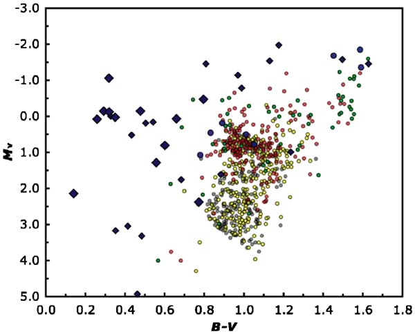
Of course, we selected our sample of giants from the Hipparcos Catalogue so that we could use the observed parallaxes and photometry to derive luminosities and effective temperatures. This allows us to plot our isolated giants together with evolutionary tracks on a Figure 12. Distribution in Download figure: versus Teff diagram, shown in Figure 12. In this diagram, the transition from rapid to slow rotation is marked by a rich population of slowly-rotating giants cooler than about log Teff = 3.7, or Teff = 5000 K. It is the sample of isolated giants at evolutionary stages cooler than this transition that we use to search for evidence of ingested planets. To guide our discussion of evolutionary stages, we once again plot the Girardi et al. (2000) evolutionary tracks for [Fe/H] = −0.2 in Figure 12, exactly as we did in Figure 8. HIP053449, an AGB giant of spectral type M5.5 III that has already completed its third dredge up (Lebzelter & Hron 2003) was not included in Figure 12, since its surface temperature determination using colors was not possible.
 versus log Teff of our isolated giants, with evolutionary tracks from Girardi et al. (2000) for mass
  and metallicity [Fe/H] = −0.2. In most of the region below the HB, stars display very little, or no rotation. Gray circles correspond to Vrotsin i < 2 km s−1, yellow to 2 to 4
  , red to 4 to 6 km s−1, green to 6 to 8 km s−1, blue to 8 to 10 km s−1, small diamonds 10 to 30 km s−1, and big diamonds to Vrot>30 km s−1. Stars in the HB region display moderate rotation, as do several stars above that region. Many stars to the left of the red giant branch in the diagram are still rapid rotators, as is expected, since for these stars "rotational braking" (Gray 1989) has not yet occurred.

Some interesting patterns at relatively slow rotations near our detection threshold are apparent in Figure 12. Stars with masses in the range 1.0–1.4 Figure 13. Enlargement of Figure 12, displaying the region around the HB. The position of the moderate rotators in the clump matches very closely the position of stars in the HB according to the evolutionary tracks for various masses and solar metallicity (Girardi et al. 2000). Open circles stand for Vrotsin i < 2 km s−1, yellow for 2 to 4 km s−1, red for 4 to 6 km s−1, green for 6 to 8 km s−1, and blue Vrotsin i>8 km s−1. A number of moderate rotators can be seen to the right of the line of first dredge-up, denoted by the red and blue dashed lines, for [Fe/H] =0.0 and [Fe/H] = −0.2, respectively. This result suggests that there is an exchange of angular momentum with a rapidly spinning core at the time of first dredge-up. The red and blue dotted lines denote the zero-age HB for the same metallicities. The arrows denote the three stars whose rotation rate is unusually high, and may require some additional spinning-up mechanism, such as planet ingestion. We used stars in the highlighted regions to perform a statistical test, showing that the two subsamples belong to different rotational velocity distributions. We infer that HB branch stars rotate moderately faster than stars with similar physical parameters on their first ascent. Dotted lines delimit the three regions of the diagram that we used for our statistical analysis (see text). The region delimited by the black dashed line includes a subsample of stars in close proximity of the two rapidly rotating clump giants. Download figure: start their climb up the giant branch with little or no detectable rotation; most of these stars show less than 2 km s−1 of rotation, while only a few are in the range 2–4 km s−1. When the first dredge-up line is crossed (Girardi et al. 2000), several stars that are unambiguously on the first ascent of the giant branch show excess rotation of up to 6.3 km s−1. An expanded plot of this region of the diagram is shown in Figure 13; the locus of first dredge-up is plotted for [Fe/H] = 0.0 (dashed red line) and [Fe/H] = −0.2 (dashed blue line). If this transition is real, it suggests that the first dredge-up transfers significant angular momentum from a spinning core to the observable outer layers. Our determinations of rotational velocities for stars near first dredge-up should be checked using a Fourier analysis of spectra with higher signal-to-noise ratios and better spectral resolution, to make sure that the macroturbulence is being handled correctly and that detailed abundance analyses show evidence of elements and isotopes brought to the observable surface by the dredge-up. If such investigations confirm that the first dredge-up corresponds to increased surface rotation, it would support the idea that the stellar cores are rotating rapidly. The idea that the cores of solar-mass stars spin rapidly is controversial (cf. Demarque et al. 2001; Thompson et al. 2003).
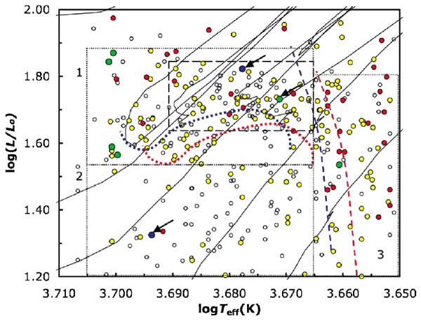
When we move up from the region below the red clump, where stars are unambiguously on the first ascent of the giant branch, and into the core helium burning region of the HR diagram, where the post-tip evolutionary tracks overlap the first-ascent tracks, we note that several of the giants show hints of modest amounts of excess rotation, with values up to 5.3 km s−1 (and two outliers show even faster rotation). Although we cannot tell whether stars in this ambiguous region are first ascent or post-tip, we can show that the velocity distributions are statistically different in the two highlighted regions: one region for unambiguous first-ascent stars and the other for ambiguous stars where the evolutionary tracks overlap. We performed a Kolmogorov–Smirnov (K–S) test on two groups of stars. One group comprised stars with 3.665 < log Teff < 3.705 and Figure 14. Histogram showing the distribution of isolated giants as a function of rotational velocity in region 2 of Figure 13. Few stars have any measurable rotation. There is one clear outlier, HIP 35253, whose Vrotsin i = 9.9 km s−1. This is a candidate for the planet ingestion mechanism discussed in the text. Download figure: Figure 15. Histogram showing the distribution of isolated giants as a function of rotational velocity in region 1 of Figure 12. This distribution is statistically different from that of region 2, as shown by a K–S test that we performed on the two samples. Several stars have 2 Download figure: Figure 16. Histogram showing the distribution of isolated giants as a function of rotational velocity in region 3 of Figure 12. This distribution is statistically different from that of region 2, as shown by a K–S test that we performed on the two samples. A possible explanation of the difference in the two samples, both containing stars on their first ascent to the giant branch tip, is that as stars undergo the first dredge-up their envelope exchanges angular momentum with a rapidly rotating core. Download figure: , below the HB, while the other comprised stars with 3.665 < log Teff < 3.705 and
  , at the approximate location of the HB (see Figure 13). Figures 14 and 15 are histograms of the two distributions, displaying the number of stars as a function of the observed Vrotsin i. The difference between the two distributions is significant to p < 10−3. We then repeated the K–S test but using stars in a group of first ascent giants to the right of the dredge-up line in place of the HB stars. This third group of stars is within the region with 3.650 < log Teff < 3.665 and
  , as displayed in Figure 13. The corresponding histogram is Figure 16. Once again, the two distributions are found to be significantly different, with p < 10−3.
 km s−1, and six stars have Vrotsin i>6 km s−1. Four of these more rapid rotators are located on the far left of region 1, while two are in the middle of the HB.
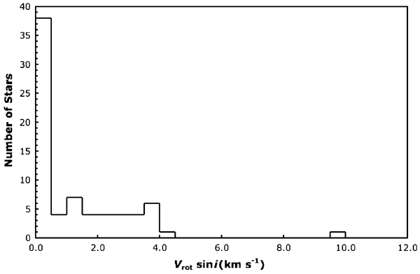
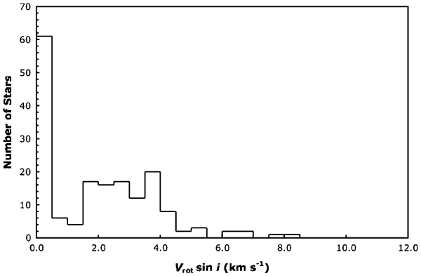
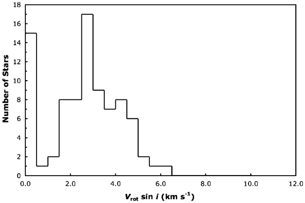
Assuming it is real, what could be the source of this excess rotation for stars near the red clump? Is this rotation related to the mechanism involved near the first dredge-up line? Alternatively, could this modest excess rotation be the net result of planet ingestion near the red giant tip, as modified by subsequent evolution and loss of mass and angular momentum? If ingested planets are the source of excess rotation, then we might expect that some stars near the red giant tip should show more rotation than others, depending on the mass of the planet and the size of the orbit, and therefore the amount of angular momentum deposited. We do see luminous giants with more line broadening, but we are cautious about assigning this to excess rotation for two reasons. First, we are unsure of the macroturbulence corrections for the most luminous stars. In particular, we note that our synthetic spectra do not match the observed spectra as well for the reddest and most luminous stars as they do for less extreme giants. Second, we note that we do not see as much excess line broadening for the most luminous stars in our sample in contrast to the result found by Carney et al. (2003) for a metal-poor sample of red giants. It is not clear whether this difference is real or a result of some systematic effect. For example, the Carney et al. metal-poor sample contains more stars that are extremely luminous and red. This is a natural consequence of that fact that our sample of solar-neighborhood stars was selected to lie closer to the Sun than 100 pc and thus contains almost no examples of stars that are intrinsically rare. Also, the luminous metal-poor stars are bluer than the corresponding giants in our solar-neighborhood sample, and thus may not have undergone as much rotational braking. The transition from rapid to slow rotators for supergiants is less well defined than for clump giants, as noted by Gray & Toner (1986, 1987).
In our sample of isolated giants, we found only four outliers that have excess rotation. One of these (HIP 103144) has Vrotsin i = 76.1 km s−1 and has been classified as an FK Comae star (Bopp & Stencil 1981). The source of the very rapid rotation of FK Comae stars is not well understood. One possibility is common-envelope evolution with a substellar companion, but only if the mass of the companion is less than about 20 MJ (Livio & Soker 1984). For more massive companions, mass transfer from the evolving giant onto the companion may save it from a common-envelope death spiral.
A second outlier (HIP 35253), with Vrotsin i = 9.9 km s−1, is located below the red clump and presumably is on its first ascent of the giant branch. Its rotation rate is 5.8 km s−1 faster than all the other stars of similar mass and evolutionary stage. HIP 35253 is the outlier in Figure 14. The Hipparcos Catalogue reports that HIP 35253 has a visual companion with a separation of 172 ± 4 mas and 0.7 mag fainter, corresponding to a projected separation of 15.6 AU. The CfA velocities show a hint of acceleration over the 3 years of coverage, which could easily be the result of orbital motion around the visual companion. The velocities show no evidence for short-period variations, so excess rotation due to tidal forces from a nearby stellar companion in a hierarchical triple system appears to be ruled out.
The final two outliers are both located in the red clump, and thus have ambiguous evolutionary histories. In Figure 17, they lie more than 2.4 km s−1 beyond all the other stars in the same region of the H–R diagram, with rotation rates of 8.4 and 7.7 km s−1 for HIP 36896 and HIP 81437, respectively. HIP 36896 also has a visual companion according to the Hipparcos Catalogue, at a separation of 198 ± 4 mas and 0.4 mag fainter. In this case, there is a combined visual and speckle orbit (Hartkopf et al. 1989) with P = 213.1 ± 5.8 years and e = 0.693 ± 0.007. For this star, the CfA velocities also show a hint of acceleration over the 3 years of coverage, but no sign of short-period velocity variations that might be attributed to a close companion. HIP 81437 clearly shows slowly-changing velocity variations over the 4 years of CfA observations, without covering a full orbital period. Harris & McClure (1983) published 17 velocities for HIP 81437, obtained over a period of 3 years starting in 1979, and they also show a slow velocity variation. Together, the two sets of velocities suggest that the orbital period may be about 9 years with only modest eccentricity. Adding in a few earlier velocities from the Lick, Mount Wilson, and Dominion Astrophysical Observatories did not lead to an unambiguous orbit. Again, there is no sign of short-period velocity variations.
Figure 17. Histogram showing the distribution of isolated giants as a function of rotational velocity in the dashed bounded area within region 1 of Figure 13. This sample contains stars in close proximity to the two clump outliers HIP 36896, with Vrotsin i = 7.7 km s−1 and HIP 81437, with Vrotsin i = 8.4 km s−1. As in the case of HIP 35253, one may explain the unusual rotational velocity of these two stars by invoking planet ingestion. Download figure:
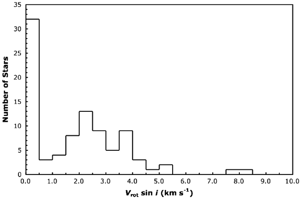
A possible explanation for the anomalous rotation of these stars is ingestion of planets. What minimum mass would a planet have to have in order to spin up these stars to the observed rotation rate? Conservation of angular momentum at the time of ingestion leads to the following expression:
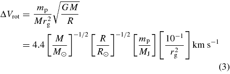
for the difference between the initial rotational speed of the star and its value immediately after ingestion. In this simplified calculation, we assumed that the angular momentum of the planet of mass mp is imparted to an envelope of angular momentum J = IΔVrot/R, where the moment of inertia is I = r2gMR2 and we chose r2g = 10−1 for simplicity (Siess & Livio 1999a). Note that, even though the angular momentum contributed by a planet scales like  , the resulting
  because of the linear dependence of the stellar angular momentum on the stellar radius.
Let us assume that all four of these rapidly rotating stars are on their first ascent of the giant branch. For the minimum amount that the rotation rate has increased for each star, we take ΔVrot to be the difference between the measured value of Vrotsin i minus the value for the fastest nonoutlier with comparable physical properties. We find minimum ingested planet masses of mp ≳ 2.8MJ for HIP 36896, mp ≳ 2.4MJ for HIP 81437, mp ≳ 4.5MJ for HIP 35253, and mp ≳ 40 MJ for HIP 103144. There are two other effects that ensure that these estimates are lower limits for first ascent stars, namely there may have been further evolution to larger size after the ingestion event and stellar winds may have carried some of the angular momentum away from the envelope.
If the two clump stars are in their HB phase instead of first ascent, they would have reached a maximum radius R ≃ 120  at the red giant tip. A planet ingested during the final stage of the ascent to the giant tip could impart a large amount of angular momentum to the star, proportional to the square root of the semimajor axis of its orbit. For the HB case, we get mp ≳ 1 MJ for both HIP 36896 and HIP 81437.
In summary, the ingestion of a planet of even a few Jupiter masses could provide the observed excess rotation for first ascent giants, and a mass close to Jupiter's would work for post-tip giants. However, more massive ingested planets would be required if mass loss after the tip carried away significant angular momentum, or if stellar winds were important.
6. SUMMARY
We report new rotational and radial velocities for 761 giants chosen from the Hipparcos Catalogue to lie within 100 pc of the sun. The velocities are based on spectra obtained with the CfA Digital Speedometers. We present new orbital solutions for 47 binaries, 13 of which are without a previously published orbital solution. We also combine new data with old measurements to update 23 orbits, and we use published data but modern software to update another four orbits. For the 75 binary systems with giants and with orbital solutions that we analyzed, all of orbits with periods shorter than 20 days have been circularized, while about half the orbits with periods in the range 20–100 days still show significant eccentricity.
We derived effective temperatures, luminosities, and radii using published photometry combined with the Hipparcos distances. We investigated macroturbulence as a function of effective temperature and luminosity using stars with published values based on spectroscopic studies at high spectral resolution and with a high signal-to-noise ratio. We then corrected the spectral line broadening measured with the CfA Digital Speedometers to remove the effects of macroturbulence statistically as a function of effective temperature and luminosity. To look for patterns in rotational velocity as a function of evolutionary stage, we identified a subsample of isolated giants where the stellar rotation should not have been affected by tidal interactions with a stellar companion. We confirm the well-known result that giants hotter than about spectral type G0 to G3 rotate rapidly, while our rotational velocities for most of the cooler giants are less than 2 km s−1.
Several giants that are just past the first dredge-up line, in a part of the luminosity versus effective temperature diagram where they must be on the first ascent of the giant branch, show rotational velocities that are just a few km s−1 higher. Perhaps this excess rotation is the result of transfer of angular momentum from spinning stellar cores to the observable surface layers. Another pattern is that giants in the red clump tend to exhibit more rapid rotation than their progenitors on the first ascent, again by just a few km s−1.
Three of our isolated giants have Vrotsin i values in the range 7.7–9.9 km s−1 and are outliers in the distribution of rotational velocities. Two of these giants fall in the red clump, while one is clearly on the first ascent of the giant branch. All three are members of long-period binaries with separations that are too large for tidal forces to be important now. We conclude that the excess rotation of these three giants could be the result of ingestion of a giant planet or brown dwarf.
We thank Bob Davis for maintaining our radial-velocity data base and Joe Zajac and Joe Caruso for obtaining many of the observations at the Oak Ridge Observatory. We also thank Bruce Carney and Dimitar Sasselov for their comments on the paper and John Laird, Guillermo Torres, Tsevi Mazeh, and Sören Meibom for useful discussions. This publication makes use of data products from the Two Micron All Sky Survey, which is a joint project of the University of Massachusetts and the Infrared Processing and Analysis Center/California Institute of Technology, funded by the National Aeronautics and Space Administration and the National Science Foundation. This research has made use of the SIMBAD database, operated at CDS, Strasbourg, France.
Footnotes
- *
Some of the results presented here used observations made with the Multiple Mirror Telescope, a joint facility of the Smithsonian Institution and the University of Arizona.