
ABSTRACT
The La Silla-QUEST Low Redshift Supernova Survey is a part of the La Silla-QUEST Southern Hemisphere Variability Survey. The survey uses the 10 deg2 QUEST camera installed at the prime focus of the 1.0-m Schmidt Telescope of the European Southern Observatory at La Silla, Chile, and utilizes essentially all of the observing time of the telescope. The QUEST camera was installed on the ESO Schmidt telescope in 2009 after completing a 5 year variability survey in the northern hemisphere using the 1.2-m Oschin Schmidt telescope at Palomar. La Silla-QUEST started science operations in 2009 September. The low redshift supernova survey commenced in 2011 December and is planned to continue for the next 4 years. In this article we describe the instrumentation, software, operation, and performance characteristics of the survey.
Export citation and abstract BibTeX RIS
1. INTRODUCTION
Type Ia supernovae have received much attention lately as calibratable standard candles for use in cosmological studies that have led to the discovery of the acceleration of the expansion of our Universe (Riess et al. 1998; Perlmutter et al. 1999). To carry these cosmological studies to an increased level of precision several surveys have gathered samples of higher redshift supernovae such as ESSENCE (Woods-Vasey et al. 2007) and SNLS (Sullivan et al. 2011). Other surveys are planned or now operating to gather larger samples of high redshift supernovae, such as PanSTARRS (Kaiser et al. 2010), DES (Bernstein et al. 2012), LSST (LSST DESC 2012) and the proposed space mission WFIRST (Green et al. 2012). The scientific motivation for carrying out a large scale survey for low redshift supernovae is to obtain a similarly large sample of well-studied Type Ia supernovae below a redshift of 0.1. Such a survey complements the high redshift surveys in several ways:
- 1.A large sample of low redshift supernovae is needed to anchor the Hubble Diagram at low redshift. A sample comparable to the size of the high redshift sample would reduce the error obtained on the cosmological parameters by as much as a factor of 2.
- 2.A well-studied sample of low redshift supernovae increases our confidence that we understand these important distance indicators that play such an important role in cosmology. In particular, the low redshift sample can lead to establishing subclasses of Type Ia supernovae with more uniform properties and to finding other features of Type Ias, such as ratios of the strength of spectral features (Bailey et al. 2009), that can further reduce the intrinsic spread in the magnitudes of the supernovae and thus improve the precision of the cosmological measurements.
Here we describe the instrumentation, search software, and operations of the La Silla-QUEST (LSQ) Low Redshift Supernova Survey, which uses the 10- deg2, 160-megapixel QUEST camera (Baltay et al. 2007) installed at the prime focus of the 1.0-m Schmidt telescope of the European Southern Observatory (ESO) at La Silla, Chile. The QUEST camera was installed on the ESO Schmidt telescope in 2009 after completing a 5-year, northern-hemisphere variability survey in 2008 using the 1.2-m Oschin Schmidt telescope at Palomar. At Palomar, this camera was the discovery engine for the Supernova Factory (Aldering et al. 2002; Kerschhaggl et al. 2011), leading to the measurement of more than 200 Type-Ia spectrophotmetric light curves. The camera was also used to discover the dwarf planets in the Kuiper Belt (Schawmb et al. 2011), to characterize the variability of quasars (Bauer et al. 2009a, 2009b, 2009c), and to measure the effect of gravitational lensing on quasar variability (Bauer et al. 2012).
The LSQ supernova survey is part of a broader LSQ Southern Hemisphere Variability Survey (Hadjiyska et al. 2012), which includes a southern-hemisphere survey of the Kuiper Belt (Rabinowitz et al. 2012), a study of RR Lyrae variable stars (Vivas et al. 2008; Zinn et al. 2013, in preparation), a search for tidal disruption events, a study of quasar variability, and a search for other unusual transients (Rabinowitz et al. 2011; Hadjiyska et al. 2013). From 2009 to 2011, the survey concentrated on the KBO and the RR Lyrae searches and on laying down reference images in preparation for the supernova search. The supernova survey started in 2011 December and is planned to continue for the next 4 years. LSQ uses essentially all of the observing time of the telescope.
Section 2 of this article describes the instrumentation used for the LSQ survey and § 3 describes the survey strategy. Section 4 describes the software and databases necessary for detection and characterization of supernova. Section 5 presents an analysis of the survey performance. Finally, § 6 describes ongoing programs at other observatories to follow-up the LSQ discoveries with photometric and spectroscopic measurements.
2. INSTRUMENTATION
2.1. The ESO Schmidt Telescope
The ESO Schmidt telescope has a 1.0 m entrance aperture and a focal length of 3 m at the prime focus where the camera is located. It has an optical configuration similar to the Palomar Schmidt telescope. The ESO Schmidt had been out of active operation since 1998, so the entire control system had to be updated. This required a complete replacement of the controlling electronics for both telescope axes and the focus mechanism, including servo amplifiers, encoders, the controlling computer and control software. Limit switches were installed to better control and monitor the rotation of the dome and the opening and closing of the dome shutter.
With the new telescope control system (TCS) it is possible to run the telescope in a fully robotic mode, similar to the previous operation of the Palomar/QUEST survey (Baltay et al. 2007). Before a night's observations commence, observing scripts are prepared at Yale and transmitted via the internet to the control computer at the telescope, where a master scheduling program automatically sequences the telescope pointings and the camera exposures. This automation is essential for enabling the operation of the survey every clear night of the year. The operator of the 3.6 m telescope at La Silla can monitor and control the opening and closing of the Schmidt dome via a web interface to ensure that the dome is closed in case of inclement weather.
The scheduling program prioritizes the telescope exposures during the night based on the positions of the scheduled fields, the number of exposures required per field, and the scheduled observing intervals. After each observation, the program assigns a new priority to each field based on its location in the sky, the number of scripted exposures that have already been completed, and the amount of time remaining to complete the required exposures. For example, if the telescope dome opens late because of clouds early in the evening, the program skips the observations of any fields that have already set, or will set too soon to complete the scripted exposures. The program also skips any field closer than 15° to the Moon. Fields that have already been observed at least once, and that are awaiting additional exposures, have higher priority than fields that have not yet been observed. The scripting procedure also allows particular fields to have higher priority if requested, as for example follow-up fields for new discoveries.
2.2. The Large Area QUEST Camera
The QUEST camera was designed and fabricated at Yale University in collaboration with a group from Indiana University for initial operation at the Palomar Schmidt telescope. Because of the similarity of the ESO and Palomar Schmidt telescopes, the QUEST camera could be moved from Palomar to La Silla without any modifications to the front end optics (which is both a field flattener lens and the vacuum window of the camera dewar), the CCD array, or the camera dewar.
A detailed description of the camera is given in a previous publication (Baltay et al. 2007). The main features of the camera are summarized here, in Table 1. The focal plane of the 161 Megapixel camera consists of 112 CCD devices arranged in 4 rows, with 28 CCDs each. The array covers 3.6 × 4.6 degrees, with an active area of 9.6 deg2 (8.7 degrees if we exclude the inoperative CCDs). The CCDs have 600 × 2400 pixels, each 13 × 13 microns. With the 3 m focal length of the telescope this corresponds to 0.88 arcsec/pixel. The CCDs, fabricated by Sarnoff Corporation, are thinned back-illuminated devices with a quantum efficiency of 95% at 6000 Å.
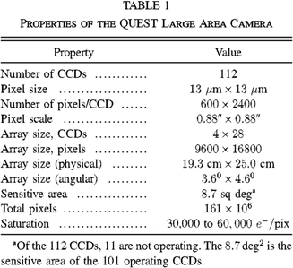 |
The layout of the CCDs on the focal plane of the camera is shown in Figure 1. The rows are labeled A, B, C, and D. Each CCD is 8.76' in the north-south direction and 35' in the east-west direction. The gaps between adjacent CCDs in a row are 1.2' and the gap between rows is 25'. The survey typically takes pairs of exposures dithered by 30' in the east-west directions to cover the gaps between the rows (additional dithers in the north-south directions are used for the Kuiper Belt survey). There are 11 CCDs which are nonoperative for various reasons (shown as blank areas with an X in Fig. 1).
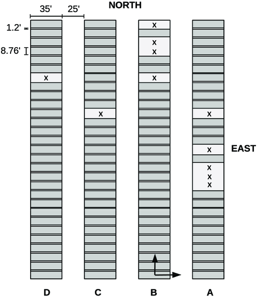
Fig. 1.— Layout of the 112 CCDs in the QUEST camera. Blank areas represent the locations of non-functioning CCDs. Vectors indicate the direction and amplitude of position offsets used to dither the imaging.
There are three improvements implemented in the La Silla survey compared to the operation at Palomar. The cooling system (to keep the CCDs to ≃120°C) no longer relies on a liquid nitrogen system that consumes significant amounts of liquid nitrogen. Now, two 60 watt cryogenic coolers are used that require essentially no maintenance for most of the year. The second change is an improvement of the readout electronics that reduces some of the noise in the images. And third, the La Silla survey uses a single wide-band filter that covers roughly 4000–7000 Å, as shown in Figure 2, along with the Gunn u, g, r, and i filters. The cutoff above 7000 Å eliminates fringing due to some strong atmospheric emission lines at red wavelengths. The cutoff below 4000 Å reduces scattered moonlight.
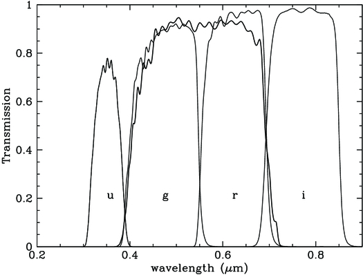
Fig. 2.— Transmission of the wideband filter used in the La Silla-QUEST Survey compared to the Gunn u, g, r, and i filters, without taking CCD quantum efficiency or atmospheric absorption into account.
2.3. Data Transfer from La Silla
The QUEST camera generates ∼50 gigabytes of compressed data per night. Originally there was insufficient internet bandwidth from La Silla to the USA to transmit that volume of data electronically to keep up with the acquisition rate. To overcome this hurdle, in collaboration with the HPWREN group of U.C. San Diego (Braun et al. 2000), LSQ designed and implemented a private high speed radio link over a 100 km direct line of sight from La Silla to the Cerro Tololo Observatory using 2-m diameter dish antennas at both ends. This radio link achieves a transmission rate of 20 Mb/s which is sufficient to transfer all of the data in real time. The receiving antenna at Cerro Tololo is connected to a high-speed internet backbone to the US that does not represent a limiting factor.
3. SURVEY STRATEGY
3.1. Cadence and Exposure Time
The sensitivity to variable objects comes from covering the same area of sky repeatedly with a 2 day cadence, i.e., area A is covered on the first night, area B on the second, repeat area A on the third, repeat area B on the fourth, and so on. Similar to other surveys (SNF, SNLS), we use an unbiased rolling search (i.e., the search does not target specific galaxies), repeating observations of most of the fields in these two sets for several months. Once a particular field has been observed multiple times in good conditions, a reference image of the field can be made. Subsequent observations of the field can then be processed by our search pipeline using these reference images for comparison. On a monthly basis we update the search pattern, dropping old fields setting in the west and adding new fields rising in the east.
To discriminate against asteroids, cosmic rays, and other rapidly varying phenomena a given area is covered twice each night with about a 2 hr separation. An exposure time of 60 s, with a 40 s readout and telescope slew time, is used for the supernova search, which is sufficient to detect supernovae up to a redshift of 0.2. In this way the survey covers up to 1500 deg2 twice per night.
The observations are carried out in pairs of exposures displaced by 30' in the RA direction to cover the gaps between the rows of CCDs. This provides a full coverage of the sky except for the small gaps between adjacent CCDs. The overlapped pair of exposures covers 4.5° in RA and 4.0° in decl. and is defined as a "field." A grid of fields, with spacing of 4.0° in RA and 4.5° in decl. is defined over the full area of the sky and observations are always carried out in these defined fields. The definition of these fields is the same as what was used in the Palomar-QUEST survey.
The exposure time and the search cadence chosen for the supernova survey could be varied. Longer exposure times would allow the search to go deeper, and thus discover supernovae earlier, at the expense of less sky coverage. Increasing the cadence interval would allow the search of more sky area, and thus more supernovae discovered. But this would be at the expense of finding supernovae somewhat less early since the signature of an early supernova is a nondetection on the previous observation of the same area of the sky. Our exposure times and cadence could be varied depending on the demands of future followup programs.
3.2. Search Area
The search fields covered on any given night are determined based on the following constraints: each field must be greater than 15° from the galactic plane, and between +25 and -25° decl. to allow follow up from both the northern and the southern hemispheres. However, fields farther south are also surveyed to avoid the galaxy where it crosses the equator. All survey fields must be observable for 60 days at an airmass less than 2 to allow discovered supernovae to be followed through their entire light curves. No observations are made closer than 15° to the moon. Each lunation, a survey simulator is used to choose the search fields based on these constraints, with fields already observed in previous lunations given highest priority.
The observation of a supernova is the result of a pixel-by-pixel subtraction of a reference image from each new observation of a given area of sky. The reference images are constructed by coadding seven previous observations of the given area. The reference images are typically a few weeks to a month older than the discovery observations, at times before the explosion of the supernova of interest have occurred. As time goes on the areas observed are gradually moved east. Reference images for the new areas are continuously constructed and updated as the search progresses.
The LSQ survey serves both a supernova and a Kuiper Belt Object (KBO) search. While all of the KBO observations can be used in supernova search, the KBO survey requires a significantly different cadence and much large search area (see Rabinowitz et al. 2012 for a detailed discussion). Half of the available dark time is dedicated to the KBO search, with all of the remaining time given to the supernova search.
4. SOFTWARE AND DATABASES
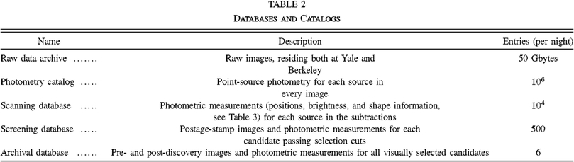
The raw data arrives at both Yale and Berkeley in close to real time. As soon as the data arrives a sequence of programs are automatically executed to process the raw data. These consist of a pre-processor, a subtraction program, and a selection procedure. The data resulting from various stages of this processing are stored in a variety of databases. Figure 3 presents a flowchart of these programs and their relation to the databases, which are summarized in Table 2.
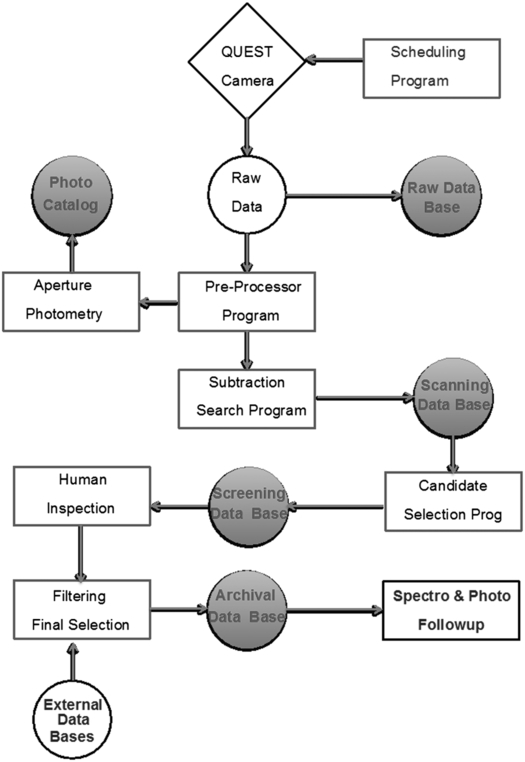
Fig. 3.— A flowchart showing the sequence of processes and their relation to various databases (see Table 2) used in the detection of supernovae in the La Silla/QUEST survey.
 |
 |
4.1. The Pre-Processor
The raw image data are corrected for nonuniform bias, dark frames, and flat fields using twilight flats and dark frames that are acquired nightly. Bias corrections are determined from overscan pixels in the images. SExtractor (Bertin & Arnouts 1996) is used to detect objects and calculate their positions in the CCD coordinates. Astrometry is carried out using the Astrometry.net software package (Lang et al. 2010) relative to field stars listed in the USNO-B1.0 catalog (Monet et al. 2003). For the supernova search this program is run automatically as soon as the raw data starts arriving, under Yale control, using the NERSC computing cluster at Berkeley.
The output of SExtractor for all observations is stored on a Photometric Object Catalog. This catalog is used for quality checks as well as for searching for transients other then supernovae, such as RR Lyrae variables.
4.2. The Subtraction Program
The subtraction program carries out the pixel-by-pixel subtraction of the reference images from the new discovery image to isolate supernovae and other variable candidates that have increased in brightness since the time of the reference image. The program is based on the subtraction program developed for the PTF survey (Nugent 2013, in preparation) but was modified and tuned at Yale to be suitable for the LSQ. For each newly acquired image (Inew), the pixels of the corresponding reference image are shifted and scaled as necessary to produce an adjusted image (Iref) for which the point sources have central pixel coordinates closely matching the corresponding sources in Inew. Here we use "scamp" (Bertin 2006) and "swarp" (Bertin et al. 2002) to calculate and perform the transformations. Iref is then convolved with an optimal spatial filter and subtracted from Inew to produce a difference image (Isub) with minimal residual signal. Here we use "hotpants"5 to perform the subtraction, with the adjustable parameters to the program initially tuned by trial and error tests on LSQ images with artificially introduced transients. For each residual source in Isub and for each corresponding source at the same location in Iref and Inew, the astrometric position, aperture magnitude and error, and other diagnostic parameters are measured using SExtractor and other programs. All positions and magnitudes are calibrated with respect to the USNO-B1.0 catalog.
Any slight mismatch in the astrometry, normalization, or the PSFs will result in fake transient candidates in the subtraction of the images of bright nonvariable stars. This is the source of the most serious background in the supernova search.
The subtracted images are then processed by SExtractor to find the candidates for transients and to calculate their magnitudes and full-width at half maximum (FWHM). Both the astrometric positions and the photometric magnitudes are calibrated with respect to the USNO-B1.0 catalog. The resulting sources in the subtracted images with a signal-to-noise ratio larger than 5 are entered on the Scanning Data Base. There are typically tens of thousands of such candidates each night.
4.3. The Supernova Candidate Selection Process
4.3.1. Computer Selection
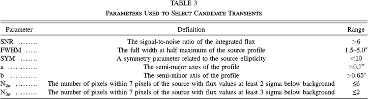
The Candidate Selection Program uses the Scanning Database as input and its function is to remove the fake candidates due to bad subtractions. For each source in the subtracted images, the program measures a variety of parameters (see Table 3) that help distinguish between real objects and artifacts. Inaccurate astrometry or mismatched PSFs that lead to positive flux artifacts in the subtractions are usually characterized by rotationally asymmetric PSFs accompanied by significantly negative flux excess (undershoots). Therefore a symmetry parameter and counts of the number of undershoots more significant than 2σ and 3σ are calculated. Another cause of noise artifacts are cosmic ray trails in the detectors which typically result in images that are smaller than the normal PSF. To discriminate against these artifacts, the semi-major and semi-minor axes of the sources image are measured. Even in well-subtracted images, very bright stars (∼mag 15 or brighter) can leave a residual source due to a few percent error of the relative normalization of the reference image. Such features can appear as real transients. To remove these artifacts, measurements are made of the position, magnitude, and FWHM of the sources in the reference images.
To originally discriminate true transients from noise artifacts, a set of selection criteria were chosen and tuned to achieve a high rejection of background while keeping a large fraction of the real sources. This was achieved by adding a large number of artificial supernovae sources into the raw image data near galaxies with redshifts between z = 0.03 and z = 0.08, as identified using the Sloan Digital Sky Survey catalog. Near each galaxy, the image was altered by adding the signal of a fake source having a flux profile identical to a randomly chosen, isolated star in the same image. Source intensities where chosen to match the expected value for a Type Ia supernova 10 days before peak at the redshift of the corresponding galaxy. The positions of the artificial supernovae relative to the center of the host galaxies were chosen randomly, but with a distance weighted by the cataloged intensity profile of the respective host galaxy.
The raw images containing these artificial supernovae were then processed through the subtraction and candidate selection programs just like the real data. The fraction of the artificial supernovae that were then selected was used to tune the selection criteria. After several rounds of tuning, we found the parameter values listed in Table 3 to be most effective in selecting candidates. To eliminate the detection of many variable stars, we also modified the selection program to reject candidates coincident with sources in the reference images that have stellar profiles and brighten by less than 2 mag. We also require all sources to be detected twice in one night. Figure 4 shows the resulting detection efficiency (fraction of artificial supernova detected) versus brightness and distance to the galaxy.
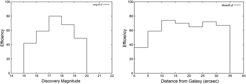
Fig. 4.— The supernova detection efficiency vs. discovery magnitude (left) and vs. angular distance from the center of the galaxy (right) determined from the detection of artificial supernovae introduced into the data.
4.3.2. Human Screening
The candidates selected by the Candidate Selection Program are added to a screening database. While the selection program reduces the number of spurious subtractions by a large factor, it still passes typically many hundreds of candidates each night. To eliminate most of the remaining bad subtractions, a human scanner examines postage stamps of the reference image, the new discovery image, and the subtracted image for each these machine-selected candidates. A typical set of such postage stamps are shown in Figure 5. In the reference image the galaxy intensity seems to vary smoothly, but the new image shows a bright spot, which shows up as the supernova image in the subtracted image. Based on a visual assessment of such images, the screener selects typically a few dozen candidates a night as probable true transients.
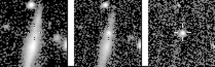
Fig. 5.— Postage stamps of the reference image (2011 November), the new discovery image (2011 December 31) and the subtracted image for supernova LSQ11ot.
4.3.3. Filtering
Filtering is the last step in selecting the supernova candidates for follow-up. This is a final assessment of the visually-selected candidates, based on their record of previous variability and cross-checks with external astronomical catalogs (SDSS, NED, the MPC asteroid database, Vizier, etc.). The assessment also utilizes previous QUEST observations of the search field containing each the candidate. Based on this history, many candidates can be clearly rejected as not supernovae (e.g., noise artifacts, variable stars, asteroids, AGN). The remaining candidates, about half a dozen a night, are then listed on the final Archival Database that is available to all of the follow-up collaborators in the Low Redshift Supernova Consortium.
5. PERFORMANCE CHARACTERISTICS OF THE SURVEY
Since the start of the LSQ supernova survey in 2011 December, the spectroscopic follow-up streams have been getting started. Therefore the spectroscopic screening and typing of the supernovae have not been up to full capacity. Nevertheless some of the performance characteristics of the survey are starting to emerge.
5.1. Areal Coverage
As discussed above, the supernova survey covers a selected area of the sky twice each night. In a clear 8 hr night we can take 288 60 s exposures (with a 40 s readout), or 144 dithered exposure pairs covering 18 deg2 each. This gives an ideal upper limit of 2600 deg2, or 1300 deg2 covered twice. The distribution of the actual areas covered twice per night in 2011 December is shown in Figure 6. Note that the fields counted in this figure were observed on nights dedicated to the supernova search. Nights which are shared with the KBO search have less area for supernova discoveries. Finally, the weather during the winter months from June to August at La Silla is often less favorable for observing, with frequent cloud cover, humidity, or high winds interrupting the observations.
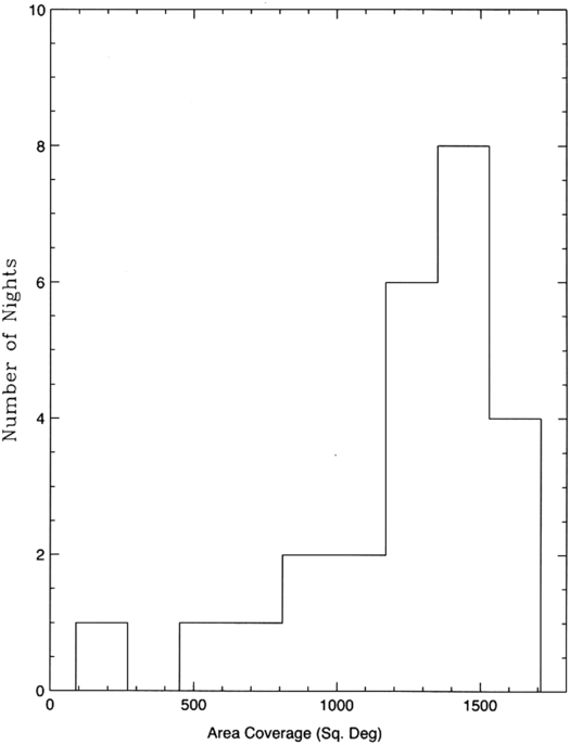
Fig. 6.— Distribution in the area covered twice per night in 2011 December.
The total area covered in the survey from 2009 September to 2012 August is shown in Figure 7, with the color coding indicating the number of times that area was visited. The areas with the least number of repeated observations (blue) are the KBO search fields, which are normally observed 3 times on one night and not repeated again. The areas with the greatest number of observations (red) are the supernova search fields, nearly all concentrated within ± 25° of the equator. The median number of observations per field, including all supernova fields observed to 2011 December to 2012 August, is 60 and the total area coverage is ∼22,000 deg2.
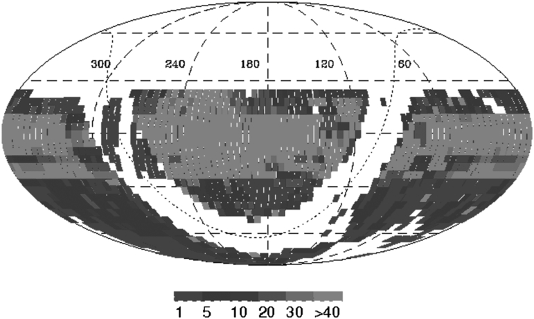
Fig. 7.— Areas covered in the La Silla-QUEST survey, between 2009 September and 2012 August. The colors indicate the number of passes in each field.
Of more importance than the total area coverage is the area multiplied by the sensitive time coverage, which is the search area factored with the time interval of continuous monitoring to ensure detection of any new supernovae. To determine this figure of merit for the fields covered by the LSQ survey we considered all fully-processed fields for which the interval between observations was less than 15 days. Since typical supernovae have rise times of ∼15 days, this ensures the detection of any new supernovae in the survey area with a pre-peak magnitude above our detection limit. Summing the area-time coverage of each field, we find our total area-time coverage was 386,000 deg2 days between 2011 December and 2012 August.
5.2. Seeing and Depth Sensitivity
The distribution of the seeing for all the observed supernova survey fields since 2010 March is shown in Figure 8, as determined by the FWHM measured for field stars near the center of the focal plane. On a night with average seeing, the FWHM ranges from 1.5'' to 3.5'' over the entire field, with median value of 1.9''. On the nights with the worst seeing (>3''), the cause of the image deterioration is usually high winds (∼40 mph) shaking the telescope rather than atmospheric turbulence. The best seeing we have seen is ∼1.2'', which is a measure of the optical distortion caused by the Schmidt and camera optics combined with the CCD resolution, not the natural seeing at La Silla.
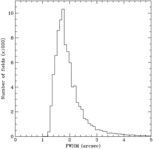
Fig. 8.— The seeing distribution with the 60 s exposures of the La Silla-QUEST supernova survey.
To determine the limiting magnitude of the supernova survey we identified a single field from the survey that was observed on a clear, dark night with average seeing (1.8'') and overlapped the footprint of the SDSS survey. We then determined the depth of the observation by measuring the fraction of SDSS stars in the field (i.e., within the boundaries of the useable CCDs in the focal plane) that were detected by our photometry pipeline as a function of their SDSS g magnitude. We define our limiting g magnitude to be the g magnitude where our completeness against Sloan is 50%. Figure 9 shows the resulting completeness versus magnitude, demonstrating a 50% completeness of the entire field at g = 21.75. The completeness is 95% at g = 20.5. To obtain an alternate view of the depth sensitivity of the survey, we took about 1000 stars measured multiple times that were distributed over the entire field of view of the camera, and plotted in Figure 10 the RMS of the measurements of each star versus its USNO R magnitude. About 2/3 of the stars in this figure had more than 30 measurements. The limiting R magnitude is 21.0 at a signal-to-noise ratio = 5.
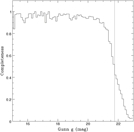
Fig. 9.— Completeness vs. Gunn g magnitude of QUEST observations of a sample of SDSS stars.
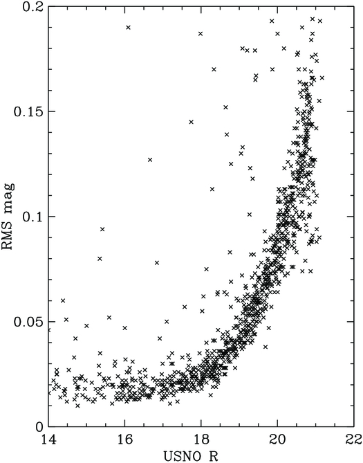
Fig. 10.— The RMS of multiple measurements of the same star vs. R magnitude.
5.3. Stability of the Flux Measurements
The repeatability or stability of flux measurements is an important feature of a variability survey. This is an especially important consideration for the LSQ survey because fields are observed in all atmospheric conditions except when there is complete cloud cover, or when it is too humid or windy to open the dome. A measure of the stability is the root-mean-square (RMS) variation of the observed brightness of non-variable stars observed on different nights and conditions. This variation is based on a relative normalization of the different measurements to each other, and not an absolute calibration to standard stars. In detail, we select field stars in each image that are common to all images, average their magnitudes, and use that average as a zero-point correction for the magnitude of each measurement. For example, Figure 11 shows the distribution of brightness measurements for magnitude 16 star observed 38 times. The RMS variation is 1.3%. As a final illustration of stability, Figure 12 shows light curves observed for three different RR Lyrae stars. These curves were assembled from observations recorded over many nights. The scatter of points on these curves is consistent with the 1.5% systematic spread in combination with the statistical errors.
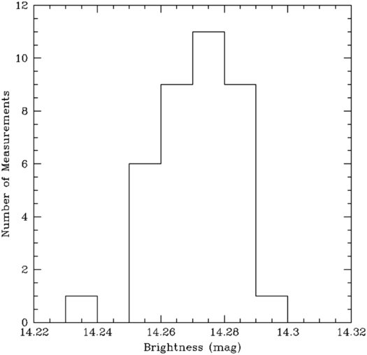
Fig. 11.— Distribution of 38 brightness measurements of the non-variable star PTF10ftx.
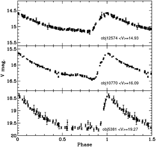
Fig. 12.— Lightcurves of a few typical RR Lyrae variable stars of magnitudes 14.9, 16.1 and 19.3 (top to bottom). Observations over many different nights have been folded into the period of the star.
Given the ∼2-day cadence of the La Silla-QUEST survey, any given supernova is observed many times. Light curves can be constructed from these repeated observations. A few typical light curves are shown in Figure 13. These light curves are in our broad survey filter (Fig. 2). To be useful for cosmology, such light curves must also be measured in standard filter systems. These are being obtained using the SWOPE telescope at Las Campanas, as discussed below.
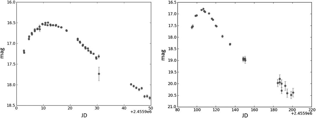
Fig. 13.— Lightcurves from the La Silla-QUEST survey for two typical Type Ia supernovae.
6. FOLLOW-UP PROGRAMS
The supernovae discovered by LSQ are followed up by several different spectroscopic and photometric programs, loosely organized as the Low Redshift Supernova Consortium (LRSC) as follows:
- 1.The Nearby Supernova Factory (G. Aldering and S. Perlmutter et al.), using the SNIFS spectrometer on the Hawaii 2.2 m telescope to take a time series of spectra for each supernova followed.
- 2.The Carnegie Supernova Project (M. Phillips et al.), using the 2.5 m Dupont telescope at Las Campanas to carry out a time series of infrared observations.
- 3.The PESSTO project (S. Smartt and M. Sullivan et al.), using the EFOSC spectrometer on the 3.5 m NTT telescope at La Silla for spectroscopic follow-up.
- 4.the 1.0 m Swope Telescope at Las Campanas (M. Phillips et al.), used to measure light curves.
- 5.1.0 m LCOGT telescopes (A. Howell et al.), use to measure light curves.
6.1. Coordination with the Follow-up Programs
As discussed above, visually selected supernova candidates are added to the Archival Database typically the day after the observations are taken. All of the collaborators doing supernova follow-up access this database to select targets for spectroscopic or photometric follow-up. Collaborators are also able to add information to this database, such as the measured redshift of a supernova or its host galaxy, the type of supernova, tables, or plots of measured spectra, and commentary. The PESSTO group, in particular, has developed procedures to ingest all the information from the Archival Database into their own web-based scheduling system (the PESSTO Marshall). Normally, the LSQ group or the follow-up teams publish the results of their observations via an Astronomer's Telegram (ATEL) within a day or two of determining a spectral type. The spectra from PESSTO are stored and publicly available in the WISEREP database (Yaron & Gal-Yam 2012).
6.2. Results from Follow-up Programs
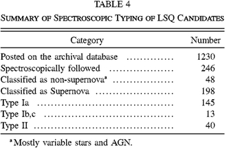
The follow-up programs mentioned above were coming into operation during the start of the LSQ supernova survey (2011 December to 2012 August). A summary of the results of the spectroscopic typing of LSQ candidates for this period is given in Table 4. These results show that 80% of the LSQ candidates that were followed spectroscopically were confirmed to be supernovae. A plot of the redshift versus the phase at discovery for 44 supernova confirmed by PESSTO is shown in Figure 14.
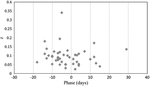
Fig. 14.— Redshift vs. phase at discovery for 44 LSQ supernovae confirmed spectroscopically by PESSTO, where phase is defined to be 0 at peak B magnitude.
 |
7. SUMMARY AND CONCLUSIONS
We have described the instrumentation, detection software, performance characteristics, and the preliminary results of follow-up programs for the LSQ low-redshift supernova survey. The program is now fully operational and performing well. While continuing to make small improvements to the survey, we are looking forward to 4 more years of productive operation. We expect to continue to discover hundreds of supernova per year, with majority being type Ia at redshift < 0.1, detected at least 5 days before peak. The most important improvement will be to push the discovery and follow up to earlier phases in the light curves. This could be achieved by further improvements in the detection software (for example, the implementation of an automated decision tree to eliminate false detections), and by more optimal coordination of the follow-up programs.
We thank Dr. Andreas Kaufer and ESO for their cooperation in making the La Silla-QUEST project possible. We also thank Dr. Gerardo Ihle and the technical staff at the La Silla Observatory for their outstanding efforts both during the installation and the operation of this survey. We thank Mark Gebhard from Indiana University for his help with the installation and commissioning of the camera electronics. We are also grateful to Dr. Hans-Werner Braun, Jim Hale, and Sam Leffler for their help in the design and implementation of the radio link from La Silla to Cerro Tololo. We acknowledge the support of our Yale colleagues Will Emmet, Tom Hurteau, and Ed Reed for their technical help without which the survey would not have been possible. This research was supported by DOE grant DE FG0 ER92 40704 and The Yale University Provosts Office.
Footnotes
- 5
For more information please see http://www.astro.washington.edu/users/becker/c_software.html.