
ABSTRACT
Ratios of the depths of appropriately chosen spectral lines are shown to be excellent indicators of stellar temperatures for giant stars in the G3 to K3 spectral type range. We calibrate five line‐depth ratios against B−V and R−I color indices and then translate these into temperatures. Our goal is to set up line‐depth ratios to (1) accurately monitor any temperature variations of a few degrees or less that may occur during magnetic cycles or oscillations and (2) rank giants precisely on a temperature coordinate. This is not an absolute calibration of stellar temperatures. We show how giant spectra can be misleading because of the complex dependences of spectral lines on metallicity and absolute magnitude as well as temperature, and it is essential to make corrections to accommodate these complications. The five line‐depth ratios we use yield precision for monitoring, i.e., detecting temperature variations, of 4 K from a single exposure. Ranking giants by temperature can be done with errors of ∼25 K but could be improved with better determinations of the metallicity and absolute‐magnitude corrections.
Export citation and abstract BibTeX RIS
1. INTRODUCTION
Although it is elementary that stellar spectra vary with temperature, the line strengths and general appearance of giant‐star spectra actually depend on several parameters, making the interpretation more complicated than one might expect. Here we explore the ratios of the depths of spectral lines as temperature indices. The lines must be suitably chosen to maximize their differences in sensitivity to temperature. Previous studies, particularly of dwarfs, have shown line‐depth ratios to be very effective, allowing variations in temperature of ∼1 K to be monitored in favorable cases (Gray & Johanson 1991; Gray 1994; Gray & Livingston 1997). This is particularly useful when studying variations during magnetic cycles or through the phases of pulsation of a variable star (e.g., Gray et al. 1996a, 1996b; Gray 2000; Kovtyukh & Gorlova 2000; Krockenberger et al. 1998; Sasselov & Lester 1990; Strassmeier & Fekel 1990). Line‐depth ratios have also been used to precisely order stars according to temperature (e.g., Gray 1989, 1994, 1995; Strassmeier & Schordon 2000). Line‐depth ratios are calibrated against effective temperature either directly or indirectly using, for example, as we do here, color indices. Therefore, there is a basic limitation on the accuracy of any temperature inferred from a line‐depth ratio (LDR) set by the accuracy of the original effective temperatures. On the other hand, if one is measuring temperature variations over time for one star or looking at temperature differences between stars, the precision can be more than an order of magnitude better than the basic calibration.
Line‐depth ratios have the advantage over residual fluxes or equivalent widths because they do not depend on the zero signal level. The zero level can be in error because of scattered light in the spectrograph or uncertain corrections for electrical baseline and/or dark leakage in the light detector. For the same reason, the spectrum can be composite and the method will still work. Although the value of the line depth does depend on placing the continuum precisely, it is not necessary to actually know the continuum level in an absolute sense; one need be consistent only between calibration and use.
There are some subtleties that have to be considered when comparing stars using LDRs. Rarely is one able to ratio two lines of nearly equal depth, and obviously even if they do have a ratio of unity at one temperature, they will not at another temperature. When the ratio differs from unity, two effects need to be watched. First, any blurring mechanism will not change both lines in the same way. For example, broadening caused by Doppler shifts of rotation or focus errors in the spectrograph fall in this category. Second, a change in line strengths will alter an LDR whenever the lines are on different parts of their curves of growth. This is the effect one faces when comparing two stars of different metallicity. Line‐depth ratios also vary significantly with stellar luminosity. The reasons are the same: Doppler broadening caused by macroturbulence increases systematically toward higher luminosity, and most lines grow stronger with declining surface gravity so that curve‐of‐growth effects again come into play.
In principle, one could calibrate the LDRs explicitly in terms of temperature, metallicity, and absolute magnitude across the whole Hertzsprung‐Russell (HR) diagram, but in this study we restrict ourselves to the less ambitious task of calibrating only the class III giants and treat the metallicity and absolute‐magnitude variations as corrections.
2. OBSERVATIONS AND MEASUREMENTS
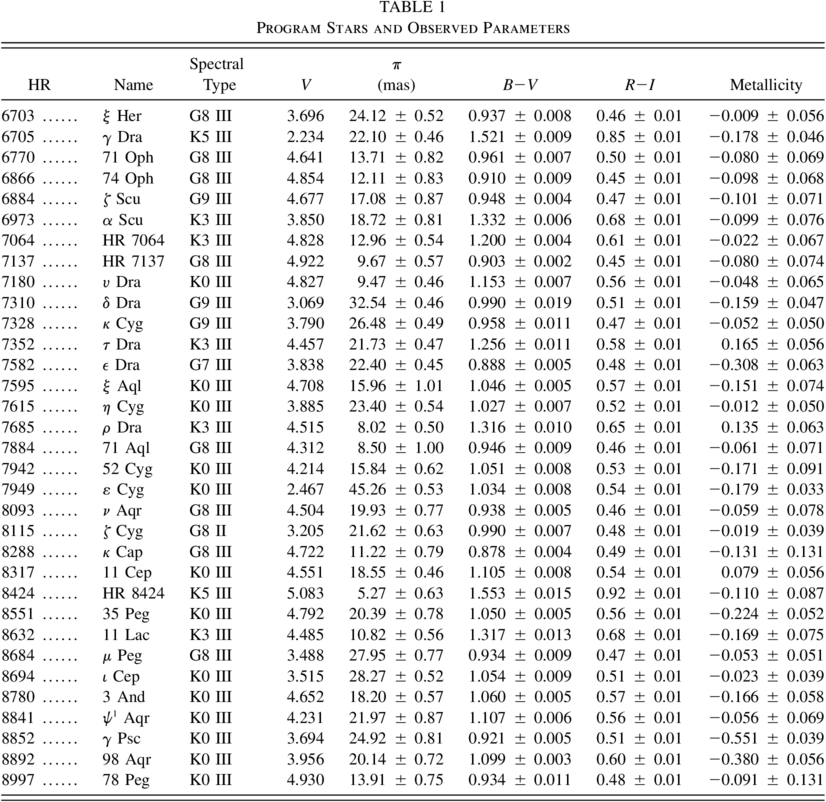
Observations of 92 class III giants of spectral types G3 to K5 were made using the coudé spectrograph with the Elginfield 1.2 m telescope at the University of Western Ontario (Gray 1986). The detector was an 1872 diode self‐scanned Reticon array. The resolving power of the spectrograph is approximately 100,000, while the usable field of view was some 70 Å centered on 6250 Å. The program stars were chosen from a much larger sample by requiring (1) a usable parallax value from the Hipparcos Catalogue, (2) low (i.e., normal) rotation rate, (3) available B−V and R−I photometry, and (4) a metallicity measurement. They are listed in Table 1, and their position in the HR diagram is shown in Figure 1. All of them are on the cool side of the rotation boundary (Gray & Nagel 1989; Gray 1989, 1992). Spectral types and R−I color indices are from the Bright Star Catalogue (5th rev. ed.; D. Hoffleit & W. H. Warren, Jr. 1996, unpublished). Visual magnitudes, V, and B−V color indices are from the Geneva Web database.1
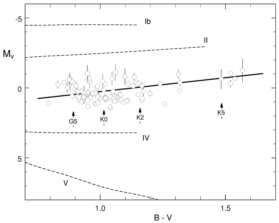
Fig. 1.— The program stars are shown in the HR diagram. The absolute magnitudes were computed using parallax measurements from Hipparcos, and the error bars reflect essentially the parallax error. Many of the error bars are smaller than the symbol size. Nominal positions of spectral classes are indicated.
 |
 |
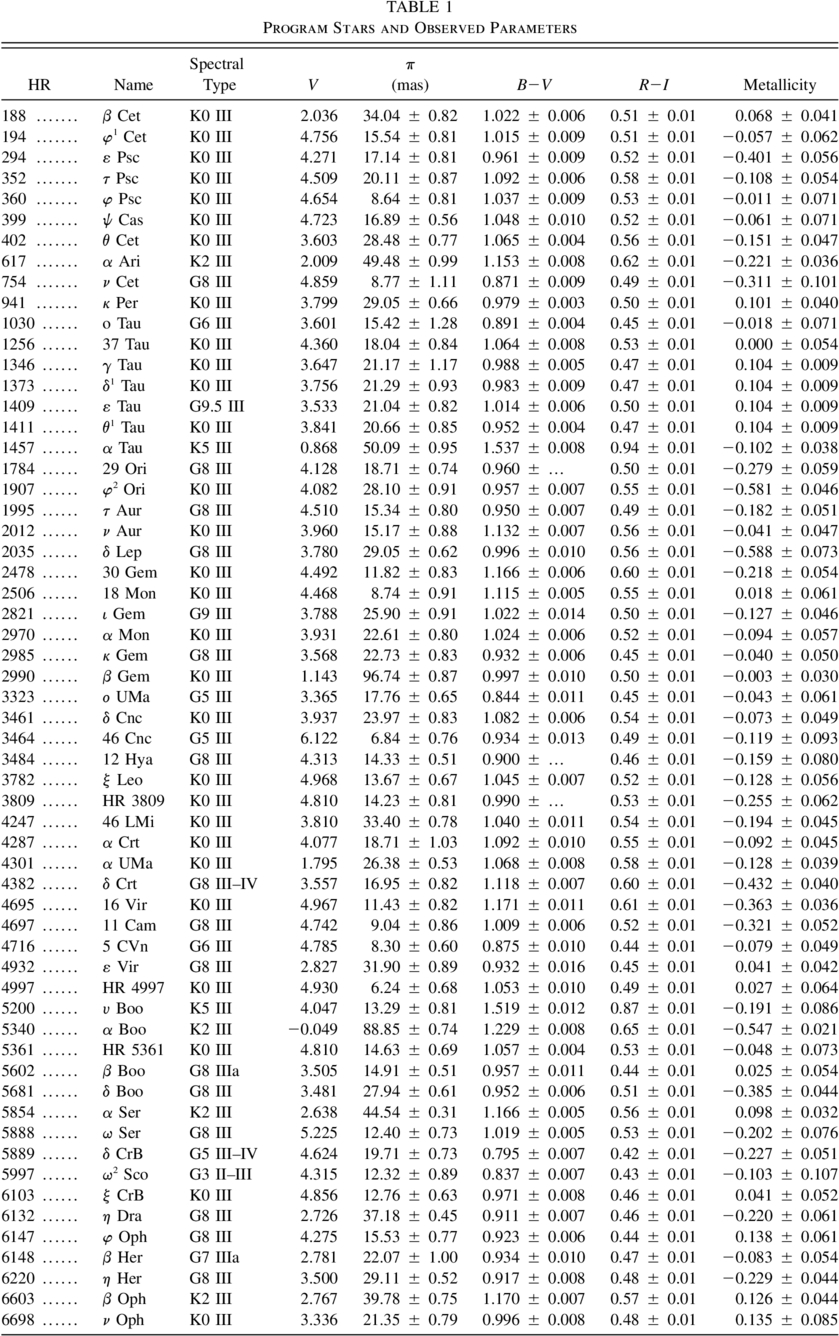
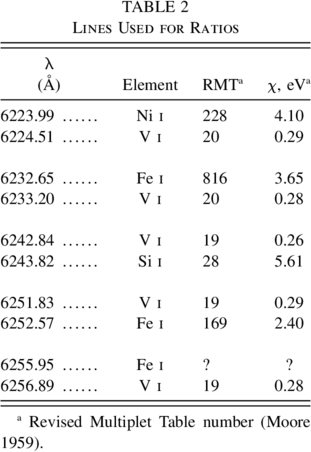
The spectroscopic data were collected between 1991 April 21 and 1999 November 6. Nominal signal‐to‐noise ratios in the continuum range from a low of 185 to a high of 905; the mean value is 585 with an rms range of 116. We used up to four exposures per star whenever possible, but for 15 of our stars, we have only one exposure. In all, five LDRs were measured on 235 exposures. The lines used are listed in Table 2. They can be located in the sample spectra given in Figure 2. The lines for each ratio are chosen to be close together in order to minimize errors in choosing the continuum. The lowest three points in the core of each measured line were fitted with a vertically oriented parabola, and the minimum of the parabola was taken to be the line depth.
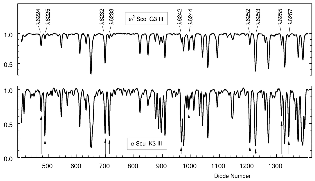
Fig. 2.— Two sample spectra are given here to show the lines used and to give some indication of their variation.
 |
Errors on the LDRs were estimated using the readout noise of the detector combined with the strength of the exposure converted to photon count. The continuum count was reduced to the line core level, and the errors of the individual line depths were combined in the standard manner to get the error on the ratio. Observed errors are often slightly larger (e.g., Gray et al. 1992). The characteristic size of the error varies with the LDR and with temperature. A typical value for the λ6252 V i/λ6253 Fe i ratio is 0.5%. A more detailed discussion of errors is given below.
3. COLOR INDICES
Since effective temperatures are determined for only a few giants, and the precision is much less than we attain with LDRs, we use color indices as an intermediary and first derive the relations between the color indices and the LDRs. We then introduce an explicit temperature calibration through the color indices as an independent step (§ 8). Observed B−V color indices were taken from the Geneva Web site, the Bright Star Catalogue (5th rev. ed.; D. Hoffleit & W. H. Warren, Jr. 1996, unpublished), and the Hipparcos Catalogue (ESA 1997). Correlations between B−V color indices and LDRs were slightly tighter with the Geneva values, and the Geneva values were therefore adopted in the subsequent analysis. The B−V values range from 0.795 to 1.553. The errors range from 0.002 to 0.019 mag, with a mean over our sample of stars of 0.0078 mag. Values of R−I were taken from the Bright Star Catalogue and range from 0.42 to 0.94. Individual measurements are expected to have statistical errors of ∼0.01 mag. In Figure 3a, we show the observed B−V plotted against the observed R−I. Expressing the deviations from the polynomial completely in terms of B−V gives a standard deviation of 0.0443 mag.
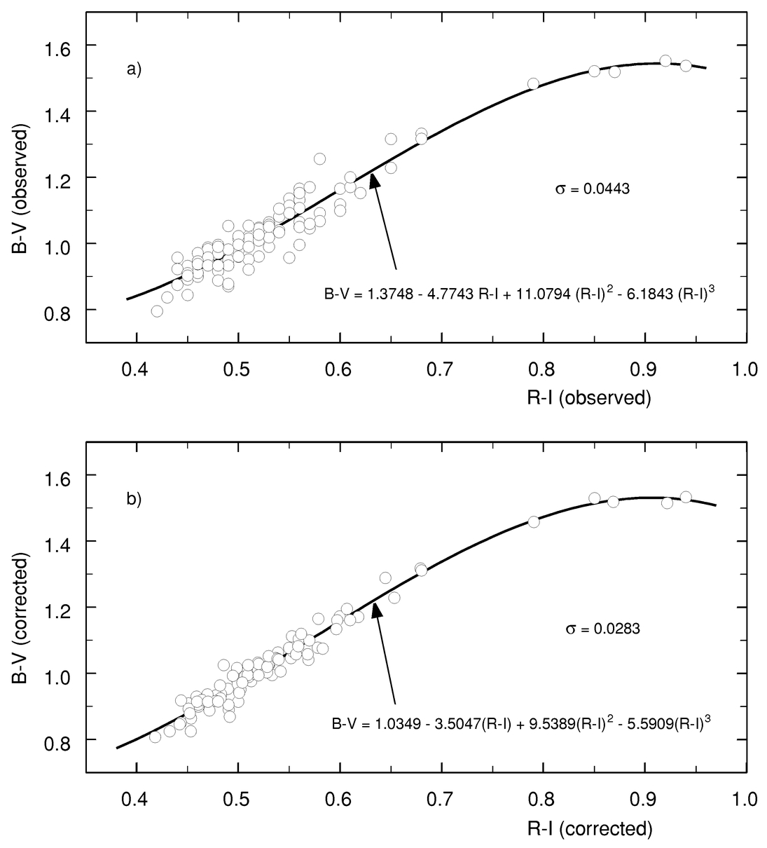
Fig. 3.— (a) Color‐color plots show scatter (beyond measurement errors) arising mainly from differences in metallicity among the program stars. B−V is affected much more than R−I. (b) The corrected indices show significantly reduced scatter.
Interstellar reddening is not expected to be large since most of these giants are relatively close. Arguments have been given that suggest extinction is essentially zero out to distances of 100 pc (e.g., FitzGerald 1970). We tried an isotropic correction using AV = 0.8 mag kpc−1 and a ratio of total to selective extinction of 3.3 based on the investigation of Henry et al. (2000). This is equivalent to Δ(B−V) = 0.2424r, where r is the distance in kiloparsecs based on the Hipparcos parallaxes. Application of this correction reduces the scatter in the B−V versus R−I plot to 0.0442, a negligible improvement. We assume the analogous correction for R−I to be even smaller and therefore neglect it.
Metallicity corrections are important for B−V, but are virtually negligible for R−I mainly because the number of spectral lines decreases toward longer wavelengths. We use this to bootstrap the corrections. Metallicity values, defined in the usual way as the logarithm of the iron abundance in the star normalized to the Sun, were taken from Taylor (1999), if available, or from Cayrel de Strobel et al. (1997). Metallicity ranges from −0.588 to +0.165 for our stars, a modest span, reflecting the fact that we observed nearby giants which are relatively homogeneous. The rms metallicity error for our 92 program stars is 0.072 based on the error estimates in the Taylor and Cayrel et al. publications. Deviations in B−V from a polynomial in the (B−V)‐(R−I) plane were plotted against metallicity. A second‐order polynomial was put through these deviations. Possible variations in the polynomial parameters with color index were investigated and found to be negligible. Application of the metallicity correction reduced the rms scatter in the (B−V)‐(R−I) plot from 0.0442 to 0.0285 mag.
We also checked for a metallicity correction in R−I. The observed R−I was plotted against the metallicity‐corrected B−V, another polynomial put through the data, and a metallicity correction sought for R−I. This correction is negligible with a correlation slope of −0.005 ± 0.020.
The final correction was for the absolute‐magnitude effect. The reference line shown in Figure 1 was taken to represent the class III giants; it was subtracted from the absolute magnitudes of the individual stars to yield a differential magnitude, ΔMV. Then the same pattern of analysis was used: deviations in B−V from third‐order polynomials in the metallicity‐corrected (B−V)‐(R−I) plane were plotted against ΔMV. There is a slight positive correlation with a slope of 0.0046 ± 0.0046, i.e., barely significant, but applying the absolute‐magnitude corrections does reduce the B−V scatter slightly from 0.0285 to 0.0283.
Figure 3b shows the final plot for the corrected color indices. The standard deviation, when expressed completely as scatter in corrected B−V, has been reduced from the original 0.0443 to 0.0283 mag. We estimate the expected scatter by combining the errors in the B−V observations, the metallicity errors (translated through the correction polynomials), and an adopted error in R−I of 0.01 mag (translated through the polynomial in Fig. 3b) under the assumption of Gaussian distributions of these errors. The result is 0.0300 mag, 6% more than the observed scatter, and sufficiently close to be considered in agreement.
Rms errors on the corrected B−V coordinate alone (R−I error not included) is 0.0193 mag. Rms error on the R−I coordinate is essentially the assumed value of 0.01 mag measurement error. These corrected color indices now represent pure temperature indices against which we compare our LDRs.
4. LINE‐DEPTH RATIOS
We select the λ6252 V i/λ6253 Fe i LDR to illustrate the analysis. The other four LDRs are treated in a similar manner. A simple plot of observed LDR versus corrected color indices shows large scatter (Figs. 4a and 4c). In these graphs we plot each of the 235 individual exposures. The standard deviations in LDR around the polynomials shown in the figure are 0.0730 for the B−V plot and 0.0766 for the R−I plot. In addition to simple measurement errors, this scatter arises because the LDR depends on metallicity and on absolute magnitude. Corrections for metallicity and absolute magnitude vary with stellar temperature, and so it is necessary to bin the data. We selected bins in R−I for both the B−V and R−I analyses.
Metallicity corrections were obtained by plotting the deviations from the polynomials shown in the upper panels of Figure 4 against metallicity for the stars in each R−I bin. A linear least‐squares fit was appropriate, as shown in the example in Figure 5a. If we denote metallicity by m, then the metallicity‐corrected LDR is given by

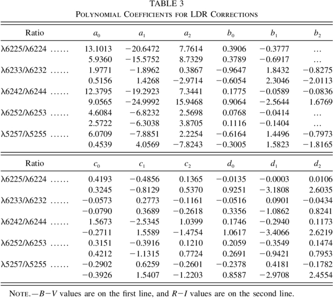
where LDR0 is the measured LDR and a and b are the slope and intercept of the metallicity correlation line. We assume that these corrections vary smoothly and continuously with LDR and color index. Plots of a and b versus bin mean B−V or R−I support this assumption. Quadratic polynomials of the form

adequately represent these variations, where C is either the B−V or R−I color index. The coefficients are listed in Table 3. The metallicity‐corrected LDR, LDRm, shows reduced rms scatter: from the original 0.0730 to 0.0311 for the B−V plot and from 0.0766 to 0.0472 for the R−I plot.
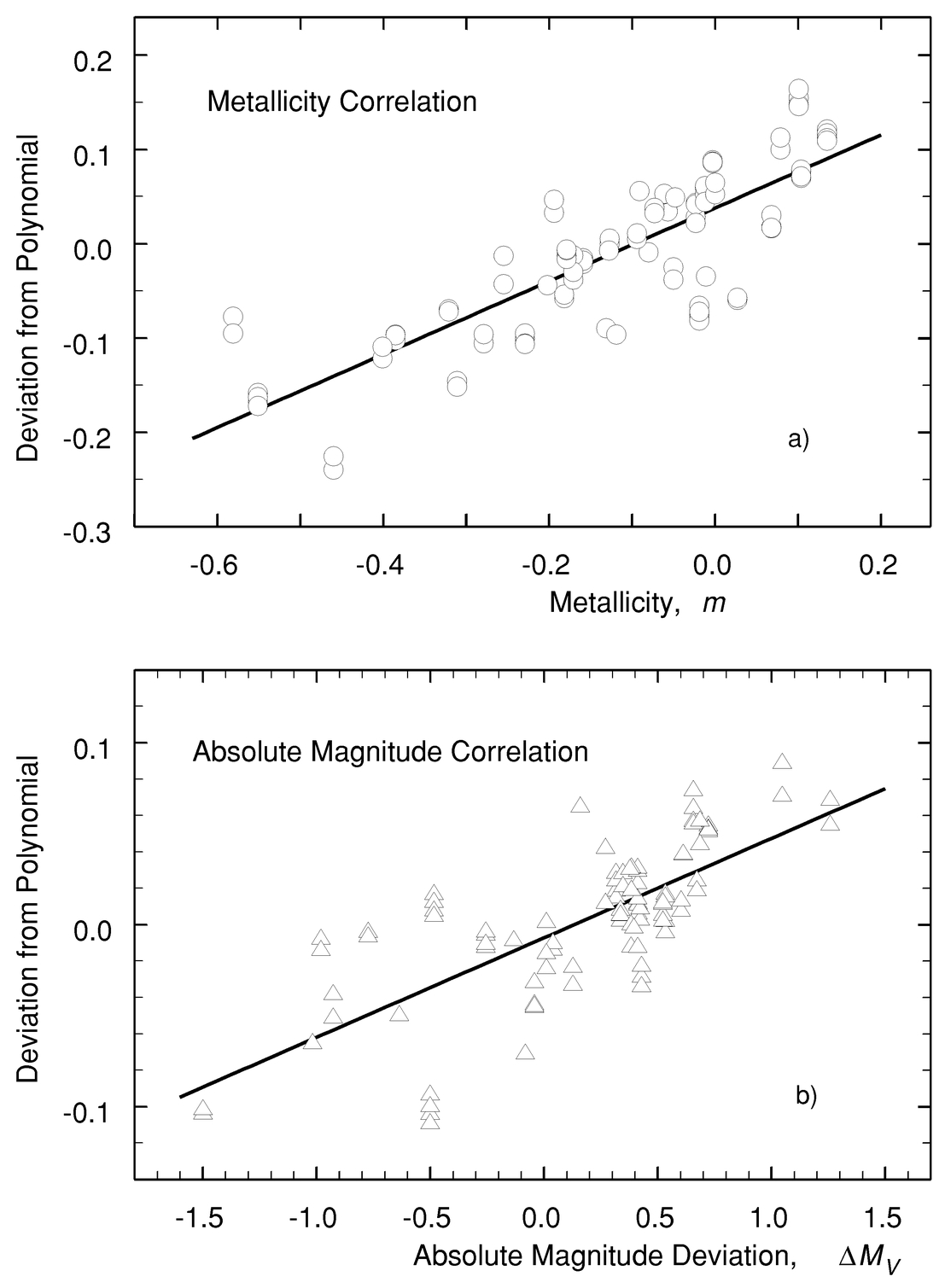
Fig. 5.— (a) An example of LDR dependence on metallicity. (b) An example of the LDR dependence on absolute magnitude. ΔMV is the deviation of each star from the luminosity class III reference line in Fig. 1. Note the difference in ordinate scale between (a) and (b). The slopes of these types of correlation plots change markedly with temperature.
 |
The metallicity correction slopes decline toward cooler temperatures. For the two LDRs involving a stronger line (λ6232 Fe i and λ6253 Fe i) the slopes are always positive, meaning that the LDR is always larger when metallicity is larger. For the other three LDRs, a reversal of slope occurs near corrected B−V = 1.1 (≈4500 K; see temperature calibration below) where the ionization of vanadium and iron are changing rapidly with temperature and where the negative hydrogen ion, which dominates the continuous opacity, is having a harder time finding free electrons.
New cubic polynomials were placed through the plots of LDRm versus color index, and the differences from these were used to determine the absolute‐magnitude dependence. We use the same reference line in the HR diagram as discussed above (Fig. 1). Deviations from this line, ΔMV, were used as the independent variable. With the data binned in R−I, straight lines were put through the plots of differences in LDRm from their polynomial representation versus ΔMV. An example is given in Figure 5b. The absolute‐magnitude and metallicity‐corrected line‐depth ratio, LDRMm, is then

in which c and d are the slope and intercept of the absolute‐magnitude correlation lines. Plots of c and d versus color index show that a quadratic polynomials suitably describe their variations,

where C represents a color index. These coefficients are given in Table 3. The absolute‐magnitude corrections are relatively small. The correlation slopes are positive in all cases, meaning that fainter stars have slightly larger LDRs. Two of the ratios, λ6233/λ6232 and λ6257/λ6255, show almost no dependence on B−V, while the others show a weaker absolute‐magnitude effect toward cooler temperatures. We presume the physical reasons for these different behaviors involves the interplay of changing ionization equilibria, macroturbulence, and rotation as they change systematically with absolute magnitude.
The lower panels in Figure 4 show the LDR corrected for metallicity and for absolute magnitude versus color index. For the λ6252/λ6253 Fe i ratio, the scatter in LDR has been reduced from the original 0.0730 to 0.0293 for B−V and from 0.0766 to 0.0366 for R−I by applying these corrections. Similar improvements in scatter is found for the other LDRs. It is therefore completely clear, both from the scale of the ordinates in Figure 5 compared to Figure 4 and from the reduced scatter of the calibration curves, that these corrections are mandatory; precise results from LDRs would be impossible without them.
The 10 such curves (two color indices for each of five LDRs) are the calibration curves, one step removed from calibrating LDR directly against temperature. Figure 6 shows the fully corrected plots for the other four LDRs. Although each has its own characteristics, they all show a nearly linear rise, and it is this portion that is useful for deriving stellar temperatures. The turnover toward redder color indices, although not well delineated with the current data, means that LDRs vary too slowly with temperature to be useful, or may even be double valued. In other words, these particular LDRs lose their effectiveness beyond about K3 III spectral type; different ratios will have to be selected for use with the cooler giants.
5. CALIBRATION CURVE ERRORS
Errors in the corrected LDRs arise from (1) LDR measurement errors, (2) metallicity errors, and (3) absolute‐magnitude errors stemming mainly from parallax errors. The derivatives of equations (1) and (3) were used to map metallicity and absolute‐magnitude errors into the LDR coordinate for each star and each ratio. All errors were assumed to be distributed in a Gaussian manner, and therefore the square root of the sum of their variances is taken to be the predicted error. For the B−V analysis of the λ6252/λ6253 ratio, the separate rms contributions to the LDR error are as follows: (1) measurement errors, 0.0040; (2) metallicity errors, 0.0198; (3) absolute‐magnitude errors, 0.0075. The metallicity error dominates, and the same is true for all five LDRs. When these errors are combined individually for each star, they predict an rms error over our program stars of 0.0225. The corresponding values for the R−I analysis of the λ6252/λ6253 ratio are (1) measurement errors, the same 0.0040; (2) metallicity errors, 0.0177; (3) absolute‐magnitude errors, 0.0071. The combined error is 0.0204, slightly better than with the B−V analysis.
The scatter in the fully corrected values shown in Figures 4 and 6 arises from this LDR error combined with errors in the abscissa translated through the slope of the polynomials into equivalent LDR errors. For the λ6252/λ6253 ratio, the predicted scatter on the B−V plot is 0.0300, compared to the observed scatter of 0.0293. The predicted scatter in the R−I analysis is 0.0332 compared to the observed scatter of 0.0366. The average ratio of observed to predicted scatter over the five LDRs is 1.27 for B−V and 1.25 for R−I, i.e., reasonable agreement but with the observed errors exceeding the expected errors.
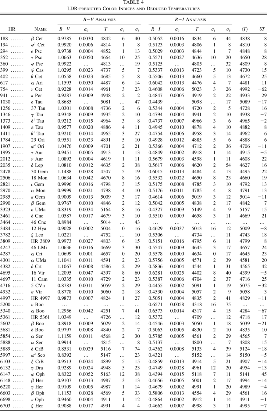
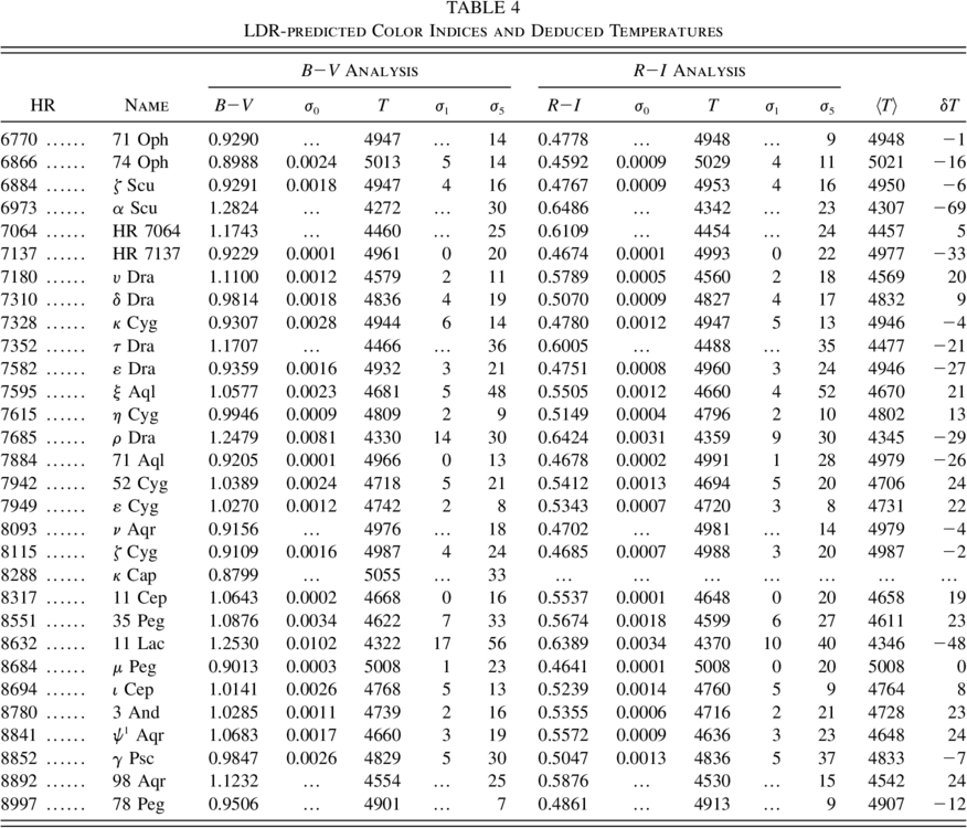
6. COLOR INDICES FROM LINE‐DEPTH RATIOS
Now that the calibration curves have been established, we turn them around and plot color indices as a function of LDRs, but we omit the portions corresponding to stars of class K4 III and cooler. Again, polynomials are put through these plots. Then each corrected LDR is read into the polynomials to yield predicted B−V and R−I. The grand mean predicted color indices for each star, i.e., the mean over the results of five LDRs and over the selected exposures for each star, are summarized in Table 4. They should not be confused with the measured values in Table 1. The LDR‐predicted color indices will be translated into temperatures in § 7.
 |
 |
The rms scatter of the exposure means around the grand mean is denoted by σ0; this represents the consistency of the exposures in yielding a predicted color index and therefore represents the precision of the process per exposure. The average σ0 over this sample of 92 stars is 1.9 mmag in B−V and 1.1 mmag in R−I. The average (over all stars and all exposures) rms scatter among the five LDRs is 12.7 mmag for B−V and 7.6 mmag for R−I.
7. CONVERSION TO TEMPERATURE
Conversion of the predicted color indices into temperature is done as a separate step because the absolute‐temperature scale is much less certain than the precision available through the LDRs. Alternative temperature scales can be introduced in this step without changing what has been done up to this point. We adopt here the temperature scale published by Taylor (1999) and plot his temperatures against the corrected color indices for those stars common to our study and his. These relations are shown in Figure 7. The polynomials shown in the figure are used to translate the mean color indices deduced from the LDRs into temperatures, and the slopes are used to translate the color‐index errors into temperature errors. The results are in Table 4. The B−V analysis and the R−I analysis appear in separate blocks. The corresponding temperatures are given in the columns headed by T, while the mean of the two is listed in the 〈T〉 column.
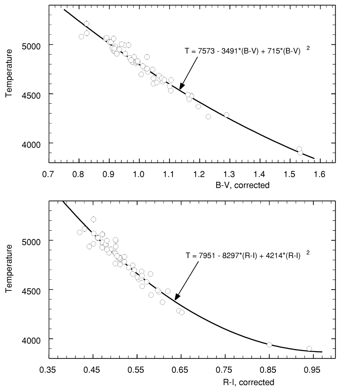
Fig. 7.— The points are for our program stars that have temperatures given by Taylor (1999). The smooth curves are used to convert the corrected LDRs to temperatures.
Naturally, if we were to use some other effective temperature calibration, such as that of Houdashelt, Bell, & Sweigart (2000) or Tej & Chandrasekhar (2000), etc., the absolute temperature from the LDRs would change accordingly. On the other hand, the ranking of stars by temperature or any time variations in individual stars that might be monitored using LDRs would not be significantly altered.
Errors associated with these results can be specified in several different ways. The first (σ1) corresponds to the precision of the five‐LDR mean and is simply σ0 times the slope of the temperature–color index curve (Fig. 7). The term σ1 is the error that is relevant when monitoring stars to detect temperature variations with time, for example, during stellar magnetic cycles. The mean observed temperature precision for this set of stars is 3.9 K per exposure, and is the same for both color indices. There is no significant variation in σ1 with color index. The predicted errors of precision discussed above in § 5, when converted to temperature units, range from 4 to 6 K across the five LDRs. If the error were to diminish with the square root of the five LDRs, then the predicted average error would be ∼2.5 K per exposure. Increasing the signal‐to‐noise ratio in an exposure or increasing the number of exposures should improve this precision, assuming the star does not vary on timescales shorter than or comparable to the exposure times.
Another measure of error corresponds to the range in LDR‐predicted temperatures within each exposure (σ5). Different LDRs give slightly different temperatures, and σ5 is a measure of this inconsistency. The mean σ5 is 21 K for B−V and 22 K for R−I. This parameter reflects the errors in polynomial fitting and the errors in the corrections that have been applied. It shows no significant variation with color index. Still another measure of error is the scatter in the calibration curves (Figs. 4 and 6). When these are appropriately translated into temperature, they range from 14 to 41 K with an average ∼25 K. As we pointed out above in § 5, the correction errors, especially those for metallicity, are much larger than the LDR measurement errors. Therefore we cannot expect much improvement in ranking errors from multiple exposures or other improvements in the LDRs.
In the final column of Table 4 we list the temperature difference between the B−V and the R−I analyses. Typical differences are ∼20 K, but Figure 8 shows that about half of this lies in systematic differences rather than random errors. This may imply that an analysis using more stars has the potential to reduce these consistency errors to ∼10 K.
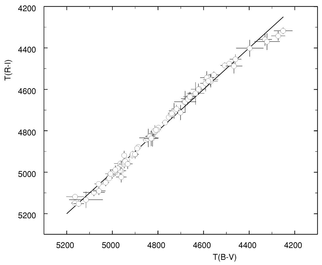
Fig. 8.— The LDR temperatures from the R−I analysis are compared to its B−V counterpart. The error bars are σ5 in Table 4 and represent the consistency of the five LDRs. The straight line is the one‐to‐one line. Small systematic deviations ∼20 K can be seen.
8. COMPARISON WITH PREVIOUSLY PUBLISHED RESULTS
Since the absolute temperatures we deduced from the LDRs depend completely on our (somewhat arbitrary) choice of temperature calibration, i.e., Figure 7, the comparisons we make here are concerned with the consistency and scatter, not with the absolute‐temperature scales. First we compare the tightness of the relation between the Taylor (1999) scale of Figure 7 and our temperatures. This is not a circular argument (even though we used Taylor's scale in our reductions) because our conversion of LDRs to temperature actually used a smooth polynomial based on Taylor's values, so in fact it is sensible to discuss this scatter. Taylor's temperatures rely heavily on the summary of McWilliam (1990). McWilliam brought together published temperatures from several different interferometer‐based studies and from energy‐distribution model‐photosphere work. His values do not involve spectral lines. In addition to McWilliam's values, Taylor also included other sources, some of which hinge on ionization temperatures, i.e., spectral lines. A straight line placed through a plot of Taylor's temperatures versus our LDR temperatures shows an rms scatter of 40 K for the 49 stars we have in common. If the error were the same in both coordinates, it would be 28 K, not far from either Taylor's error estimate (23 K for this subset of stars) or ours. McWilliam (1990) lists 84 of our program stars, and the rms scatter around a straight line in the correlation plot with our LDR temperatures is 41 K. McWilliam gives errors for several color index–temperature relations in his Table 6; the average 1 σ error is 35 K, so the agreement between his tabulations and our LDR results is very good.
Recently Strassmeier & Schordan (2000) derived temperatures for giants using LDRs. There are 33 stars in common with our study. The correlation plot shows an rms scatter of 99 K! (A 34th star in common, 5 CVn [HR 4716], was omitted because the temperature listed by Strassmeier & Schordan seems to be completely spurious, differing by almost 1000 K, a fact they noticed.) On the other hand, these authors also list temperatures taken from other published sources (including McWilliam 1990), and a correlation plot of our LDR values with these "literature" values for the same 33 stars shows much better agreement with a scatter of only 44 K. Since Strassmeier & Schordan make no allowance for the variation of LDR with metallicity or with absolute magnitude, poor agreement is not surprising. We saw in § 4 how essential these corrections are. An estimate of their size, bearing in mind that they vary widely with effective temperature, comes from the reduction in scatter resulting from applying the corrections (Fig. 4). The more the LDR differs from unity, the larger the corrections, and the typical LDR used by Strassmeier and Schordon is ∼2. From our calibration curves, this implies an increase by 2.5 times, i.e., the ∼25 K scatter we deduced for our ranking error in § 5 would have been ∼75 K without the corrections. This is comparable to the excess scatter seen in the results of Strassmeier & Schordon.
9. ADDITIONAL COMMENTS AND CONCLUSIONS
As we have seen, the appearance of spectra of giant stars can be misleading if one is not careful to take into account the effects of metallicity and absolute magnitude. With due allowance for these variables, suitably chosen LDRs make excellent temperature indices. For the G and early K giants, the five LDRs we used yields a precision for monitoring temperature variation of individual stars of ∼4 K per exposure. We expect that combining exposures and increasing the signal‐to‐noise ratio of individual exposures will allow temperature resolution of temporal variations of 1 K. Errors in ranking stars by temperature are ∼25 K, and a significant fraction of this error comes from uncertainty in metallicity determinations; we hope to improve this shortcoming in a future study.
Once calibrated, the LDR technique is purely spectroscopic and is therefore independent of interstellar reddening. Since line depths are measured downward from the continuum, the technique is not sensitive to zero‐level errors and can be used even if the spectrum is composite.
Color indices may, of course, be used to infer stellar temperatures, and it is edifying to make some comparisons. As shown in § 7, a single spectroscopic exposure yields precision equivalent to 1.9 mmag in B−V or 1.1 mmag in R−I, and ranking accuracy to 12.7 mmag in B−V or 7.6 mmag in R−I. The first set of numbers is comparable to the best high‐precision photometry (e.g., Henry et al. 2000). The second set of numbers can be compared to the errors associated with the corrected color indices of § 3: 19.3 mmag for B−V and ∼10 mmag for R−I. In other words, a single spectroscopic exposure having a signal‐to‐noise ratio exceeding ∼200 and from which five LDRs are extracted is comparable to or exceeds the photometric capability for temperature determination. Since the metallicity correction is currently the limiting factor, combining exposures or increasing the signal‐to‐noise ratio of the observations will not greatly improve the spectroscopic ranking by temperature. Tactically, the spectroscopic approach requires more reduction effort and is harder to use on fainter stars compared to photometry, but it has the important advantage of not needing photometric skies.
The LDR error of resolution corresponds to an increment of ∼0.003 of a spectral class; the ranking error corresponds to ∼0.023 of a spectral class.
It should be noted that in our sample of stars, variations arising from differences in the macroturbulence and rotation are small, largely because these phenomena vary coherently with position in the HR diagram (Gray 1988). Should one wish to investigate stars with anomalous line broadening, special care will be needed, and in some cases it may be necessary to restrict the analysis to LDRs near unity. In a similar way, variations stemming from errors in spectrograph focus could be serious for LDRs not near unity.
Where we have used the absolute magnitude as an independent variable, surface gravity, which more directly influences the photosphere, would be preferable. The confluence of evolutionary tracks in the giant region of the HR diagram results in a degree of decoupling between surface gravity and absolute magnitude. Further refinement in determining precise temperatures from LDRs may be possible. At the same time, some caution should be used because at some level each star is an individual; a general metallicity index will have to be replaced with the detailed abundance distribution for each star, even small non‐LTE effects might introduce inconsistencies, and differences in rotation rates and magnetic fields could influence the heterogeneous structure of a stellar photosphere and hence the LDRs. At what level of temperature precision these complications enter remains to be determined.
We are grateful for the financial support given to us by the Natural Sciences and Engineering Research Council of Canada. Our gratitude goes to Wayne Warren for salient comments on color indices and to the referee for suggesting improvements. We thank the observing assistants, who over many years have contributed to the accumulation of data, some of which we use in this project.
Footnotes
- 1
J.‐C. Mermilliod, B. Hauck, & M. Mermilliod 2000, http://obswww.unige.ch/gcpd/cgi‐bin/photoSysHtml.cgi?0