
ABSTRACT
We have used Hipparcos parallaxes to derive absolute visual magnitudes of G, K, and M stars with Ca ii emission line widths previously measured by O. C. Wilson. A linear relationship similar to the one derived originally by Wilson & Bappu and improved by Lutz & Kelker was found from Mv = +7 to −2. For stars brighter than Mv = -2 a substantial number of stars show Ca ii emission lines that are broader than expected from the linear fit. Most of those stars are bright giants and supergiants of type G. In appendices we show some sample Ca ii profiles and identify emission lines of Fe ii as well as the H line in some stars.
Export citation and abstract BibTeX RIS
1. INTRODUCTION
In 1957 O. C. Wilson and M. K. V. Bappu reported on the remarkable correlation between the measured width of the emission feature at the center of the Ca ii K line and the absolute visual magnitude of the star. The correlation is independent of spectral type and applicable to stars of type G, K, and M. Their original calibration was based on the Sun and the four K giants in the Hyades. Except for the main‐sequence stars there were not many additional calibrating stars with sufficiently accurate parallaxes to evaluate the dispersion about the mean relation or to extend the calibration to stars brighter than about Mv = 0.
The paucity of accurate parallaxes for luminous red giants has been largely overcome by the Hipparcos program (Kovalevsky 1998) in which parallaxes with uncertainties of near 1 mas were obtained for numerous stars. Hence, we now have 10 σ parallaxes out to 100 pc and 5 σ data to 200 pc, providing Mv‐values with uncertainties of 0.21 and 0.42 mag, respectively. Therefore, the large database provided by Wilson (1976) can be combined with Hipparcos parallaxes to recalibrate the Mv - log W0 relation, where W0 is the measured width corrected for the instrumental width. In addition, stars that appear to deviate from the Wilson‐Bappu relation may be investigated in order to understand the anomalies of their chromospheres.
2. THE DATABASE
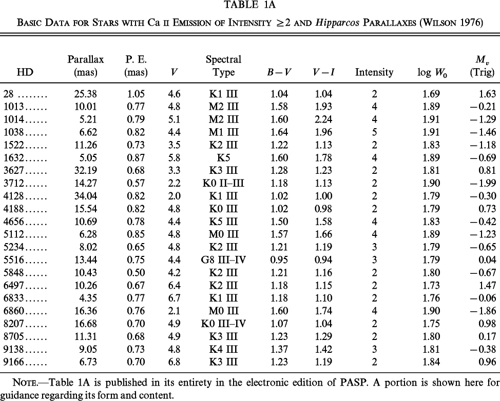
We have limited ourselves to stars with parallaxes that are at least 5 times their probable error and whose log W0‐values are listed by Wilson (1967, 1976). Other databases are available, e.g., Warner (1967) and Zarro & Rogers (1983), but the Wilson data are so much larger than the others that we decided to base our discussion on these data alone. For each star we have extracted the parallax, its probable error, V magnitude, spectral type, B−V color, and V−I color from the Hipparcos Catalogue (ESA 1997). These quantities are listed in Table 1 pasp_111_757_335tb2pasp_111_757_335tb3along with Wilson's intensity index (1–5), log W0, and the Mv‐value derived from the apparent magnitude and parallax.4 The complete data set has been used to plot Figure 1, where we show Mv plotted against log W0, the same coordinates used by Wilson & Bappu (1957). Because of the crowding we do not show the probable errors of each point in this plot.
 |
 |
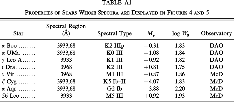 |
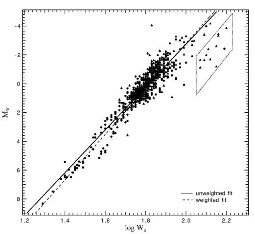
Fig. 1.— Dependence of Mv as derived from Hipparcos parallaxes on log W0. An unweighted least‐squares fit to the data is shown as a solid line. The dashed line shows a least‐squares fit with the points weighted by Π/Π. Circles represent stars with Π>10Π; triangles represent stars with 10Π>Π>5Π. Stars within the parallelogram are described in Table 2. The symbols have the same meaning in the next two figures.
At the time of Wilson & Bappu's original work accurate parallaxes were available for many dwarfs, some subgiants, and a few giants extending up to about Mv≃0. In addition the four Hyades giants were used because their distance was believed to be accurately known (but was in error by about 0.3 mag in m−M). From Wilson's data the relationship between Mv and log W0 appeared to be a straight line. Aside from one wildly deviating point and some stars with log W0>2.05, our data set can be fitted by the solid straight line, which is a linear, least‐squares fit with the parameters:
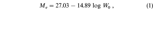
which is very similar to Wilson's (1959) calibration of

where W0 = W -18. W0 is the measured width, W, corrected for the instrumental width.
As shown in Figure 1, the linear least‐squares approximation falls above most of the points with Mv≳4.0 because the data are dominated by stars with Mv between +1 and −2. The data can also be fitted by weighting the observations by Π/Π. This adds weight to the lower luminosity stars because of their larger parallaxes. The linear fit of the weighted data is shown as the dotted line in Figure 1 and is represented by
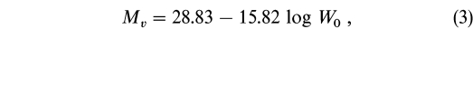
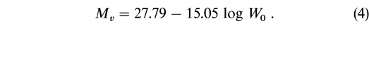
which is not very different from equation (1) and fits the fainter stars rather well. Equation (3) is closer to the linear fit of Lutz & Kelker (1975) using their corrections to the trigonometric parallaxes (Lutz & Kelker 1973, hereafter L‐K):
The linear relationships of equation (1) or equation (3) are useful from about Mv = +7 to Mv = -2. Scoville & Mena‐Worth (1998, hereafter SM‐W) have performed an analysis similar to ours using the Mg ii resonance lines observed with IUE and having parallaxes greater than 4 times their probable error. For 92 stars SM‐W find a regression line of
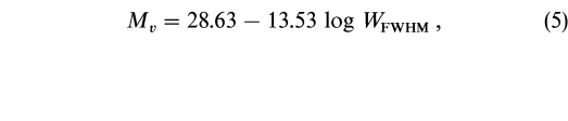
which has a smaller slope than equation (1) or equation (3). An inspection of their Figure 2 indicates that a steeper slope would better fit their data.
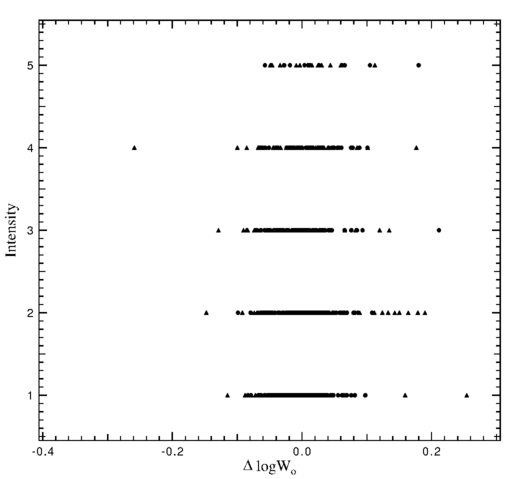
Fig. 2.— Dependence of the deviation from the mean line, Δlog W0, on Wilson's estimated intensity of Ca ii emission.
Figure 1, which includes the stars with less accurate parallaxes shown by triangles, extends the Wilson relationship only to moderately more luminous stars, but substantially to broader K line widths than used in the Wilson (1959) calibration. The reason for this is not obvious and is one of the more interesting aspects of our investigation.
A contributing cause may be the L‐K effect by which more stars are scattered into a sample defined by a limiting parallax and a limiting probable error than are scattered out of the sample. The application of the L‐K effect to luminous stars is not straightforward. The L‐K formulation is designed to handle a spherical distribution of stars. A problem arises for giants more luminous than Mv≃ -2, whose distribution is likely to be somewhat flattened, since such stars should be increasingly rare at heights above about 100 pc from the Galactic plane. The uncertainty in Mv for stars with Π/Π≃5 should be somewhat asymmetric to include the L‐K effect, which increases the uncertainty of the rarer high‐luminosity stars while leaving the uncertainty of the low‐luminosity stars largely intact. Roughly speaking, the 1 σ uncertainty must be near 0.4 mag, and a few errors as large as 0.8 mag are expected. Such uncertainties fail to account for many of the stars with log W0>2.05 because their luminosities must be raised 2–3 mag to fit a linear extension of the relationship shown in Figure 1 and expressed in equations (1) or (3). It appears that many stars in Figure 1 with log W0>2.05 show anomalously wide Ca ii emission. The simplest external sources of distortion of the Ca ii profiles, circumstellar and interstellar absorption, serve only to narrow the emission profile. The wide profiles must be intrinsic to the stellar chromospheres.
3. SOME CORRELATIONS
Rather than looking at the scatter about the mean lines in Figure 1 (or eqs. [1] or [3]) as the uncertainty in Mv, let us take the astrophysical point of view of investigating the spread in measured line widths at a given value of Mv. For stars with Π>10Π the scatter introduced by the uncertainty in Π is ≤±0.2 mag, while for 10Π>Π>5Π the error is ≤±0.41 mag. However, the reader (if any) should remember that in large data sets 2 σ and even 3 σ errors will be found! Likely parameters upon which log W0 may depend are spectral type and intensity of the emission line.
First, we will look at the intensity parameter. Wilson's (1976) eye estimate of the intensity of the Ca ii emission is a useful parameter (Griffin 1998). In Figure 2 we plot the deviation of log W0 from the line in equation (1) against the estimated intensity. Stars with Π>10Π are plotted with different symbols from stars with 10Π>Π>5Π. There appears to be no significant correlation of Δlog W0 with intensity.
Second, we look at the possibility of deviations as a function of spectral type. We show this in Figure 3. An asymmetry is evident with a tendency for stars of type G to show positive deviations, i.e., to show Ca ii lines that are wider than predicted. The discrepant G stars are generally drawn from the sample with 5Π<Π<10Π. One might surmise that the larger uncertainty in Mv is responsible for the deviation of these stars from the linear relationship; however, an uncertainty in Π of 2 σ leads only to an uncertainty in Mv of 0.42–0.82 mag. The deviations are not random but are almost entirely toward lower luminosity or larger values of log W0 than expected. The deviations in Mv are up to about 3 mag, which cannot be due to random errors, nor can the L‐K corrections be responsible.5 Clearly, the larger error limit permitted more distant stars into the sample thereby extending it to include G stars of luminosity class II and Ib. Their Ca
ii profiles are intrinsically wider than expected from the linear Wilson‐Bappu relation.
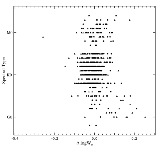
Fig. 3.— Dependence of Δlog W0 on spectral type
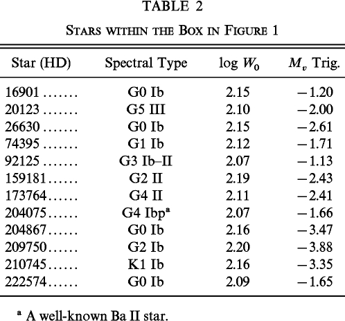
In Table 2 we show the characteristics of all the stars within the box shown in Figure 1. Clearly, the stars with broader lines than predicted by their Mv‐values are mostly G stars of luminosity class Ib and II. This is the realm of the "hybrid" stars that show both low‐ionization (e.g., Fe ii, Si ii, Mg ii) and high‐ionization (e.g., C iv and Si iv) chromospheric emission lines (Dupree 1986). Three stars from the Zarro & Rogers (1983) database fall in this region. They are of types F8 II, K3 Ib, and M1 II.
|
4. SUMMARY
We have shown that Hipparcos parallaxes of G, K, and M stars showing the Ca ii K line in emission allow an accurate calibration of the Wilson‐Bappu effect from Mv = +7 to −2. For luminosities fainter than Mv = +7, additional measurements of intrinsically fainter stars of the Ca ii emission lines are necessary. For stars brighter than Mv = -2 the dispersion around the regression line of Mv against log W0 increases and is asymmetric with numerous stars, mostly of type G and luminosity class Ib or II, showing K line widths that are significantly broader than expected from a linear fit of the Wilson‐Bappu correlation. The wide range of Ca ii line widths in stars with Mv between −1 and −4 provides an interesting problem in the structure of stellar chromospheres.
L. M. P. was supported with a scholarship from Fundacion Gran Mariscal de Ayacucho, and G. G. was supported by the Kennilworth Fund of the New York Community Trust. We thank M. Shetrone for obtaining the spectrum of one star for us, and both R. P. Kraft and R. F. Griffin for useful comments on the manuscript.
APPENDIX A: SOME HIGH‐RESOLUTION PROFILES
As a quick reconnaissance of some line profiles we have obtained high‐resolution spectra of a few giants. Two data sets are represented. The first was obtained at the McDonald Observatory with the 2.7 m telescope, echelle spectrograph and a 2048 × 2048 CCD. The resolution is about 60,000. The second set was secured at the Dominion Astrophysical Observatory (DAO) with the 1.2 m telescope, coudé spectrograph, long camera, and a 1024 × 1024 CCD. The resolution is approximately 40,000. Both sets cover both the Ca ii H and K lines and provide profiles with higher resolution and much greater S/N than used by O. C. Wilson in his pioneer work. Sample profiles are shown in Figures 4 and 5, and the stars are described in Table A1.
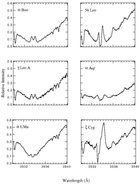
Fig. 4.— Sample profiles of the Ca ii K line. Note the apparent emission features at 3936.0 and 3938.3 Å due to Fe ii in some stars.
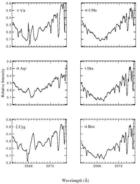
Fig. 5.— Sample profiles of the Ca ii H line and H
|
The spectra largely speak for themselves. The Ca ii emission lines are sufficiently broad and well resolved to show a central absorption feature in every star. For HD 200905 (=ξ Cyg) the violet displaced absorption core, presumably due to stellar mass loss, distorts the profile and is certainly responsible for the small log W0 measured by both Wilson and ourselves.
APPENDIX B: EMISSION BY H AND Fe ii
As part of the original work on the Ca ii lines, Wilson (1957) also noted that some stars showed emission at H as well. Our high S/N permits our spectra to show considerable evidence for H emission in several stars. In Table A2 we show the presence of H by tabulating the apparent wavelength of the hump near the wavelength of H relative to the center of the Ca
ii emission. Five stars show emission centered within 0.15 Å of the wavelength of H.
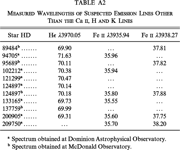 |
An inspection of our spectra also shows that for some stars there is a hint of emission near 3936 and 3938 Å. Mira variables often show emission lines at the 3935.94 Å line of Fe ii, multiplet 173 and at 3938.27 due to Fe ii multiplet 3. There is an indication of both these lines in the spectra displayed by Wilson & Bappu (1957, Figs. 9 and 10) for stars more luminous than about Mv = 0.0. Our measured wavelengths of these lines are also listed in Table A2.
In summary, it appears that H emission is present in four stars, HD 89484, 95689, 124897, and 137759. The Fe ii line at 3935.94 Å is present in HD 94705, 102212, 124897, and 209750. The Fe ii line at 3938.27 Å seems to be present only in HD 209750. Four stars show a line near 3837.82 Å, which may be an unidentified line or a gap in blended absorption features. For HD 124897 (=Arcturus) the Arcturus Atlas (Griffin 1968) shows H to be clearly in emission, but the Fe ii lines are absent. This casts doubt on our Fe ii identification on the McDonald spectrum, unless the intensity of chromospheric emission in Arcturus is variable. Since the DAO spectrum did not show the lines despite its high resolution and good S/N, variability is quite likely. Additional spectra of comparable resolution and S/N, perhaps combined with spectral synthesis to handle the background absorption lines, are needed to confirm the reality of these emission features in individual stars. The reality of H emission illustrated by Wilson (1957, Fig. 5) can hardly be questioned.
Footnotes
- 4
Table 1 is divided into three sections: Table 1A contains stars with Ca ii emission index ≥2 from Wilson (1976); Table 1B contains stars of index 1 from the same source; and Table 1C contains stars in Wilson (1967).
- 5
The referee (R. P. Kraft) has called our attention to the possibility that interstellar absorption has introduced significant errors in Mv in Table 2. Of the 12 stars in Table 2, seven have EB - V≤0.03 and HD 16901 has EB - V = 0.12 (Burstein & Heiles 1982). The others have ∣b∣<10o and are at distances of 213–256 pc. For an absorption of roughly 1 mag kpc−1 for stars at low Galactic latitude the error in Mv should not be larger than 0.5 mag for any star in Table 2. The data by Neckel et al. (1980) confirm this for specific stars.