


Pump-probe gas phase X-ray scattering experiments, enabled by the development of X-ray free electron lasers, have advanced to reveal scattering patterns of molecules far from their equilibrium geometry. While dynamic displacements reflecting the motion of wavepackets can probe deeply into the reaction dynamics, in many systems, the thermal excitation embedded in the molecules upon optical excitation and energy randomization can create systems that encompass structures far from the ground state geometry. For polyatomic molecular systems, large amplitude vibrational motions are associated with anharmonicity and shifts of interatomic distances, making analytical solutions using traditional harmonic approximations inapplicable. More generally, the interatomic distances in a polyatomic molecule are not independent and the traditional equations commonly used to interpret the data may give unphysical results. Here, we introduce a novel method based on molecular dynamic trajectories and illustrate it on two examples of hot, vibrating molecules at thermal equilibrium. When excited at 200 nm, 1,3-cyclohexadiene (CHD) relaxes on a subpicosecond time scale back to the reactant molecule, the dominant pathway, and to various forms of 1,3,5-hexatriene (HT). With internal energies of about 6 eV, the energy thermalizes quickly, leading to structure distributions that deviate significantly from their vibrationless equilibrium. The experimental and theoretical results are in excellent agreement and reveal that a significant contribution to the scattering signal arises from transition state structures near the inversion barrier of CHD. In HT, our analysis clarifies that previous inconsistent structural parameters determined by electron diffraction were artifacts that might have resulted from the use of inapplicable analytical equations.
INTRODUCTION
Molecular structures at or near equilibrium have been extensively studied using static gas-phase X-ray and electron scattering.1–4 The scattering signals reflect the geometry and electronic structure of molecules and can be inverted to determine detailed molecular parameters, including bond distances and angles. As quantum mechanical systems, molecules vibrate even at absolute zero temperature, which needs to be taken into consideration for accurate determinations of the molecular structures. For thermally stable molecules near equilibrium, a Boltzmann distribution in harmonic oscillations serves as a reasonable approximation,3,5,6 but as we show here, these approximations fail when the molecular systems are far from equilibrium as is the case in thermally highly excited systems. We describe a molecular dynamics (MD) approach to derive an accurate description of molecular scattering in such extreme conditions.
The imaging of molecular structures far from equilibrium is central to the study of chemical reactions.7–9 The recent development of ultrafast-pulsed X-ray free electron lasers10 and mega-electron-volt electron sources11 has enabled measurements on molecular structures far from equilibrium. This resulted in numerous exciting findings, such as photoinduced ring-opening reactions,12–14 coherent nuclear vibrations,15,16 and photodissociation reactions.17,18 While in many systems, the nuclear dynamics starts out as a well-defined wavepacket with a structure distribution that resembles a classical system, a large amount of energy in play during the reaction typically relaxes into a hot bath as the molecule returns to a thermal state.13,19,20 A complete description of the time resolved scattering patterns therefore requires not only a simulation of the transient dynamic structure but also a model of the scattering patterns of molecules in thermally hot vibrational conditions. For polyatomic molecular systems, this includes structures that are thermally populated yet far from the equilibrium geometry.
Several effects need to be considered for molecules with large-amplitude vibrations and much has been discussed in the context of static scattering signals of thermally excited molecules. Pioneering diffraction studies showed that the distances between nonbonded atoms in linear molecules may be shorter than the sum of bond distances (Fig. 1).21–23 While small, this so-called Bastiansen-Morino shrinkage effect may be large enough to manifest itself in high quality experiments.24,25 Bartell et al. have systematically explored the effect of shrinkage on scattering experiments.26–31 The shrinkage effect exists for both harmonic and anharmonic vibrations,31 which can be ascribed to the fact that interatomic distances are not necessarily congruous with normal mode vibrations. For nonlinear polyatomic molecules, the concept of shrinkage could be generalized to a temperature dependence of the interatomic distance distributions in vibrating molecules. This could include an enlargement instead of a shrinkage of the distances between some nonbonded atoms in nonlinear molecules, as in the case of 1,3-cyclohexadiene (CHD) that is the subject of this study.

For molecules with as few as three atoms, even harmonic normal mode vibrations may result in an apparent “shrinkage” of interatomic distances compared to a rigid body at rest. In the triatomic “ABC” molecule, the AC distance shrinks when a bending mode vibration is excited.
For molecules with as few as three atoms, even harmonic normal mode vibrations may result in an apparent “shrinkage” of interatomic distances compared to a rigid body at rest. In the triatomic “ABC” molecule, the AC distance shrinks when a bending mode vibration is excited.
Treating the electron density of molecules as a sum of isolated-atom electron densities centered at the positions of the nuclei, the Independent Atom Model (IAM) expresses the scattering cross sections using tabulated atomic form factors in a convenient way.4 For rotationally isotropic, nonvibrating molecules, the Debye scattering equation for gas phase X-ray scattering is written as3
where ITh is the Thomson cross section for a free electron, Nat represents the total number of atoms in the molecule, Rij is the interatomic distance between the ith and jth atoms, and are the elastic and inelastic atomic form factors,4 respectively, for the ith atom. For harmonically vibrating molecules in a thermal Boltzmann distribution at temperature T, the formula is traditionally modified by including, only for interatomic distances, where i ≠ j, a vibrational correction,3
Here, lh,ij is the mean vibrational amplitude centered at Rij, which depends on the temperature as7
where μ is the reduced mass, ν is the vibrational frequency, h is Planck’s constant, and k is the Boltzmann constant.
The use of Eq. (2) requires care. The Rij are interpreted as the centers of the Gaussian distributions that represent the interatomic distances during vibrations. Thus, they are not always identical to the interatomic distances at equilibrium, as illustrated in Fig. 1, when large-amplitude vibrations lead to shrinkage or enlargement effects. In general, a N-atomic nonlinear molecule will have interatomic distances but only 3N-6 vibrational degrees of freedom. This implies that for molecules with more than 4 atoms, there will be redundant parameters of interatomic distances and vibrational amplitudes. The interatomic distances are not independent parameters but rather are correlated through the limited number of intrinsic vibrational modes. It may be useful to simulate a scattering pattern when all the exact Rij and lh,ij values are known, but it is problematic to extract all the Rij and lh,ij values by fitting a scattering pattern using Eq. (2).
For highly excited systems, the anharmonicity of large-amplitude vibrations adds to the complexity of expressing interatomic distances.32 Analytical solutions have been derived for relatively simple polyatomic molecules, such as CO2, H2O, and SF6, for temperatures below 1000 K.33 Unfortunately, for more complicated molecular systems with less symmetry, and for the higher temperature that often result from optical excitation, reliable approximations and values for the asymmetry constants have not been obtained. Thus, a better way of modeling scattering patterns of hot molecules is needed.
In this article, we investigate a method for modeling scattering patterns of hot molecules based on molecular dynamics (MD) simulations. With the rapid development of the computational chemistry tool set, molecular dynamics simulations are widely applied to the interpretation of pump-probe scattering experiments. For example, Minitti et al. observed the real time ring-opening molecular motion of CHD within 200 fs by performing a global fit to time-resolved X-ray scattering patterns using ab initio multiconfigurational Ehrenfest trajectories.12 A comparison of MeV electron scattering data with ab initio multiple spawning wavepacket simulations by Wolf et al. showed the subsequent conformational isomerism of 1,3,5-hexatriene (HT) following ring-opening of CHD in the subpicosecond time regime.13 It was even possible to follow the coherent vibrational motions of a molecule following electronic excitation using ultrafast X-ray scattering.16 That analysis was made possible by utilizing a large number of possible molecular structures obtained from MD simulations. Thus, we note that recent investigations of time-resolved pump-probe scattering have begun to take advantage of large-scale modeling of scattering patterns of systems that include far from equilibrium structures. Nevertheless, to date no systematic investigation of hot, vibrating molecules has been reported.
Figure 2 illustrates the method to calculate scattering patterns of hot molecules. An MD simulation creates a large number of molecular structures that include, depending on the initial energy used, structures that are far from equilibrium. The output of the MD calculation is inherently a time sequence of structures, but we disregard the temporal aspect and simply extract a large number of structures resembling the ensemble of vibrating molecules. For each of these structures, the IAM scattering pattern is calculated following Eq. (1). To simulate a scattering pattern of the hot ensemble of molecules, the average over all the individual patterns is taken. By taking the entire pool of MD structures, the method inherently accounts for all previously mentioned effects such as shrinkage/enlargement, anharmonicity, and correlation between interatomic distances. The method can be applied to molecular structures of any complexity, limited only by the ability of MD methods to calculate reasonable trajectories. In principle, the method is not limited to the IAM model, as one could also use more comprehensive codes to simulate scattering patterns for each structure from ab initio wavefunction methods.34–36 Yet, it is important to note that the method is applicable for modeling the hot ensemble after thermal equilibrium is reached, as it does not apply to the dynamic motions observed before such equilibration.

Concept of the method for modeling scattering patterns of hot molecules based on molecular dynamics (MD) simulations.
Concept of the method for modeling scattering patterns of hot molecules based on molecular dynamics (MD) simulations.
While the concepts of this article can be applied equally to X-ray and electron scattering, we have tested it on data from a time-resolved pump-probe X-ray experiment. Specifically, we explored gas-phase 1,3-cyclohexadiene and its isomer 1,3,5-hexatriene (HT) at thermally hot conditions. The interconversion between CHD and HT is an important model for electrocyclic reactions, and its motif is used in the synthesis of vitamin D in the skin upon exposure to sunlight.37 The CHD/HT system is favorable for the present investigation because optical excitation at 200 nm is followed by an electronic relaxation that dominantly leads to the vibrationally hot CHD in the ground electronic state.38 The resulting molecules are very hot (∼2870 K for CHD, assuming harmonic frequencies reported by Autrey et al.39) and undergo a thermal ring-opening reaction to HT. Because both the hot CHD reactant and the HT products are on the ground electronic surface, complications to the scattering patterns arising from the electronic excitation are avoided.40 The thermal energy enables the electrocyclic reaction on the ground electronic surface, eventually leading to an equilibrium between hot CHD and hot HT.14
EXPERIMENTAL AND COMPUTATIONAL METHODS
Femtosecond time-resolved gas-phase X-ray scattering
The experimental setup, which has been introduced previously,41 is shown in Fig. 3. The measurements were performed at the CXI instrument42 of the Linac Coherent Light Source (LCLS) X-ray free electron laser at the SLAC National Accelerator Laboratory. An ensemble of free CHD molecules at room temperature is controlled by a piezoelectric needle valve to ∼6 Torr of pressure at the interaction region. The molecules in the gas cell are excited by 200 nm optical pump pulses with ∼80 fs pulse duration, and probed by 9.5 keV X-ray pulses with ∼30 fs pulse duration that contain ∼1012 photons/pulse. The pump and probe pulses were focused collinearly onto the scattering cell with about 30 μm FWHM spot sizes for the X-rays and 50 μm for the laser. The time delay between the laser and X-ray pulses was controlled by an electronic delay stage, and the timing jitter was monitored to ∼30 fs by a spectrally encoded cross correlator43 to achieve a higher time resolution. To obtain the best signal to noise ratio, the shot by shot X-ray pulse intensity was monitored by a photodiode downstream of the scattering cell. Single shot scattering patterns are detected via a 2.3-megapixel Cornell-SLAC Pixel Array Detector (CSPAD),44 binned by the delay time between the laser pump and X-ray probe pulses. The gas cell and the CSPAD detector are in a vacuum with about 2.6 × 10⁻⁴ Torr background pressure outside the cell, mostly comprising CHD flowing out of the windowless scattering cell.

A schematic illustration of the experimental setup. The reaction of CHD is initiated with a 200 nm pump pulse, and the time-evolving molecular structure is probed via scattering using X-ray probe pulses with variable time delay. The scattering signals are recorded as a function of the momentum transfer vector (q) and azimuthal angle (Φ) using a CSPAD detector.
A schematic illustration of the experimental setup. The reaction of CHD is initiated with a 200 nm pump pulse, and the time-evolving molecular structure is probed via scattering using X-ray probe pulses with variable time delay. The scattering signals are recorded as a function of the momentum transfer vector (q) and azimuthal angle (Φ) using a CSPAD detector.
Due to the quadrant symmetry of the cos2(θ) distribution resulting from a single-photon excitation process, the angular symmetry of the 2-dimensional scattering patterns can be described by second order Legendre polynomials.45 In this case, the percent difference scattering pattern can be decomposed into an isotropic component that contains all the intrinsic molecular properties in the molecular frame and an anisotropic component that reflects both rotational and structural dynamics of the excited molecules in the laboratory frame.46 Our analysis focuses on the isotropic component because the intramolecular vibrations of excited systems are fully described by the rotationally averaged scattering patterns. The time-dependent percent difference signal is expressed as
where q is the magnitude of the momentum transfer vector, Ion(q,t) is the scattering signal at time delay t, and Ioff(q) is the reference scattering signal when the pump laser is off. γ is the excitation fraction, which was 6% and therefore low enough to minimize undesired multiphoton processes. The advantage of expressing the pump-probe scattering signal as a percent difference is that poorly characterized experimental parameters such as background signals, gas pressure fluctuations, and pixel noise are largely minimized. The decomposition into isotropic and anisotropic signals, the detector calibration, and the analysis of the measured scattering are discussed in more detail elsewhere.18
Modeling scattering patterns of hot molecules using molecular dynamics
The ground state dynamics of hot CHD and hot HT are simulated using the SHARC program47 interfaced with the electronic structure package MOLPRO.48 More than 100 000 geometries calculated from MD are extracted to represent an ensemble of hot vibrating molecules for each CHD and HT at their thermal equilibrium. The internal energy of the system is adjustable by varying the energy input in the simulation and in this case was chosen to match the laser photon energy. Equation (1) is used to calculate the scattering pattern for each extracted geometry, and these individual patterns are then averaged to yield a single scattering pattern for the hot CHD or HT at the thermal equilibrium. The sequence of the averaging steps cannot be reversed: if one were to average the structures first and then calculate a scattering pattern of the averaged structure, important information about the distribution of interatomic distances during the vibrations is lost, resulting in the absence of damping that is characteristic of scattering patterns of hot molecules.
The initial conditions for the hot CHD are sampled from Wigner distributions to account for the zero point vibrations. The 6.2 eV of excess kinetic energy, corresponding to the energy of the 200 nm photons, was randomly distributed among all degrees of freedom of the molecules. The electronic structure calculations during the molecular dynamics are performed at the SS-CAS(2,2)/6-311+G(d) level. Similarly, the initial conditions for three HT conformers (cZc-HT, cZt-HT, and tZt-HT) were sampled from Wigner distributions. The relative equilibrium energies of cZc (1.02 eV), cZt (0.81 eV), and tZt (0.69 eV), relative to CHD, were obtained at the same level of theory and are in good agreement with previously reported literature values (0.37 eV of cZc and 0.13 eV of cZt relative to tZt49). For the 6.2 eV of photon energy, the total excess kinetic energies are therefore 5.18 eV for cZc, 5.39 eV for cZt, and 5.51 eV for tZt. A total of 50 trajectories were calculated for CHD up to 5 ps. For HT, a total of 150 trajectories were calculated up to 3 ps, with 50 trajectories starting each from cZc-HT, cZt-HT, and tZt-HT, so that the energy allows the molecules to traverse the entire ground state potential energy surface. The time steps of 0.5 fs are chosen carefully to make sure that the energy is conserved during the MD calculations while keeping the computational time reasonable. It is worth pointing out that one could have started the trajectories elsewhere. Given that the energy of the system is well above the barrier heights, the energetically accessible phase-space is effectively sampled provided the potential energy surface and the amount of excess kinetic energy are reasonable. In practice, however, the equilibrium geometry is a good choice as the structure and initial energy can be predicted well at the equilibrium.
In order to calculate the percent difference patterns accurately, the reference ground state signal Ioff is important. In the current study, Eq. (2) is used to simulate the reference scattering pattern including harmonic vibrations at room temperature. The optimized structure at the SS-CAS(2,2)/6-311+G(d) level of theory is used as the equilibrium structure. A summary of several interatomic distances and structural angles are compared with previous experimental and theoretical results in Table I. The structure used here is deemed reliable as it agrees with previously reported computational and experimental results. The mean vibrational amplitudes of CHD at room temperature reported by Cyvin and Gebhardt are used for the calculation of the scattering patterns.50 These values agree well with electron diffraction data measured by Traetteberg.51
Selected interatomic distances and structural angles of CHD at the ground state equilibrium. CAS: the structure calculated in this study, optimized from SS-CAS(2,2)/6-311+G(d). Ref. 52: optimized structure by Merchán et al. Ref. 51: experimental structure from electron scattering measured by Traetteberg.
Convergence
To evaluate the convergence of the MD method for calculating hot scattering patterns, Fig. 4(a) shows the average of the inversion angles (C1—C2—C3—C4 torsional angle, see labeling in Fig. 6, inset) for different time bins in the CHD MD simulation. All simulations start with positive values of the inversion angle sampled from zero point vibrations near 42.6°, which is the equilibrium structure inversion angle. Structures at early MD run times, before equilibrium is reached, should be dominated by positive inversion angles. Once the system has thermalized, structures with positive and negative inversion angles are expected to be equally populated. The approach to thermal equilibrium can therefore be illustrated by plotting the average inversion angles as the MD calculation progresses in time. As shown in Fig. 4(a), convergence is reached around 2 ps of MD simulations. Similarly, the time dependence of the convergence in HT is examined in Fig. 4(b). Since the MD simulations for HT are initiated from three different equilibrium structures (cZc, cZt, and tZt), the difference between Φ1 and Φ3 is about 41°, as caused by the distinguishable labeling of the Φ1 and Φ3 in cZt conformers at the beginning (see labeling in Fig. 9, inset). Once the system has thermalized, the assignment of these two angles is expected to be equivalent. As shown in Fig. 4(b), convergence is reached around 1 ps of MD run time.

The convergence of the hot MD trajectories for (a) CHD and (b) HT. The inversion angle of hot CHD structures from all 50 trajectories with a 1 ps time bin centered at different time points is averaged to get the mean inversion angle shown as y axis values in (a). The Φ1 and Φ3 dihedral angles of hot HT structures from all 150 trajectories with a 1 ps time bin centered at different time points are averaged to calculate the mean Φ1 and Φ3 angles, respectively. The absolute difference between two mean angles is then shown as y axis values in (b). The center of each time bin is shown as the x axis value for each red dot in both plots.
The convergence of the hot MD trajectories for (a) CHD and (b) HT. The inversion angle of hot CHD structures from all 50 trajectories with a 1 ps time bin centered at different time points is averaged to get the mean inversion angle shown as y axis values in (a). The Φ1 and Φ3 dihedral angles of hot HT structures from all 150 trajectories with a 1 ps time bin centered at different time points are averaged to calculate the mean Φ1 and Φ3 angles, respectively. The absolute difference between two mean angles is then shown as y axis values in (b). The center of each time bin is shown as the x axis value for each red dot in both plots.
To get a well-thermalized ensemble that accurately reflects the hot CHD molecules, all the structures calculated for each time step with MD run times between 3 and 5 ps from 50 trajectories (200 000 structures in total) are extracted to be used. The resulting simulated scattering pattern of hot CHD is shown in Fig. 7(a). Similarly, for hot HT molecules, a total of 300 000 structures are extracted from 2 to 3 ps time of run time, for 150 trajectories. Those structures are used to simulate the scattering pattern of the hot HT shown in Fig. 10.
The convergence of the simulated scattering pattern with respect to the number of structures used for simulating the thermalized ensemble is further evaluated in Fig. 5. For each entry in the plots, the N structures are selected randomly from the previously extracted, well-thermalized MD ensemble (200 000 structures for CHD and 300 000 structures for HT), and the mean absolute deviation is calculated. The y axis values shown in Fig. 5 are averaged mean absolute deviations by repeating the random selection procedure 1000 times in order to minimize noise. For the relatively small CHD and HT molecular systems, it is apparent that already 1000 structures could simulate the scattering patterns of hot molecules quite nicely with relatively small deviations. This means that one could greatly reduce the computation time for small molecules or apply this method for larger molecular systems by selecting a smaller number of structures while maintaining a reasonable accuracy.
![FIG. 5. The convergence of the scattering pattern as a function of the number of structures N for the ensembles of (a) CHD and (b) HT molecules. The mean absolute deviation calculated by ∑q%ΔIN−%ΔIMD∑q1 is shown as y axis values, where MD is the converged ensemble used to simulate the scattering pattern of hot CHD [Fig. 7(a)] or hot HT (Fig. 10). The common logarithm of the number of structures N used for simulating the scattering pattern of hot molecules is shown as the x axis value.](https://aipp.silverchair-cdn.com/aipp/content_public/journal/jcp/151/8/10.1063_1.5111979/3/m_084301_1_f5.jpeg?Expires=1716900467&Signature=NLQSQpIaeWTKo4wAYcnbps4WhlTDyorqby~~bBrQ3fx14M-rJSRkq8pwKXY6rHKnAGUapj23qV48QytdTJRHY--AcyjBFUSudkb49FIrKB3nivtHDZkMwRCRhi1swMUBtYRG~dDD4dHrJ3H9VSGtmv9eL-yU2Y5BBg~vjCxY95B9HUKHZQICmXcgI6aKlki78qDlmlv9wF4lX3v3Fr2PIYuoF7Ut7u2S38rc5eUjpoCbzSLR7oYDlcU~DSPysUsiUXryMHLq11GJb15kMbaI6zk0MLZJc4nVcI5LlA9FtHomPV1KUsl-zgVQqyrO88HiHAzcNAB~UoGlaaoclm9dag__&Key-Pair-Id=APKAIE5G5CRDK6RD3PGA)
The convergence of the scattering pattern as a function of the number of structures N for the ensembles of (a) CHD and (b) HT molecules. The mean absolute deviation calculated by is shown as y axis values, where MD is the converged ensemble used to simulate the scattering pattern of hot CHD [Fig. 7(a)] or hot HT (Fig. 10). The common logarithm of the number of structures N used for simulating the scattering pattern of hot molecules is shown as the x axis value.
The convergence of the scattering pattern as a function of the number of structures N for the ensembles of (a) CHD and (b) HT molecules. The mean absolute deviation calculated by is shown as y axis values, where MD is the converged ensemble used to simulate the scattering pattern of hot CHD [Fig. 7(a)] or hot HT (Fig. 10). The common logarithm of the number of structures N used for simulating the scattering pattern of hot molecules is shown as the x axis value.
RESULTS AND DISCUSSION
The detailed analysis of the experimental scattering data has been reported in a previous publication.14 Unlike the previously observed ultrafast ring-opening dynamics at lower excitation energies,12,37 with 200 nm excitation to the 3p Rydberg state, 76% ± 3% of the molecules relax to vibrationally hot CHD in the ground electronic state with a time constant of 208 ± 11 fs. A thermal ring-opening reaction on the ground electronic state surface is then activated and an equilibrium between the hot CHD and HT is eventually reached, with the ring-opening and ring-closing time constants determined to be 174 ± 13 ps and 355 ± 45 ps, respectively. By describing this thermal reaction scheme using kinetic equations and treating the scattering patterns of the initially electronically excited 3p CHD*, hot CHD and hot HT as adjustable parameters,14 the pure hot-molecule scattering patterns have been extracted from the 2-dimensional fits of the experimental data (Expt. curves in Figs. 7(a) and 10, uncertainties are given in 1σ).
The theoretical scattering signals of the hot CHD and the HT isomers were calculated using the MD methodology. Since detailed structural measurements exist for CHD, including vibrational amplitudes, a direct comparison of the signals calculated using the traditional approach [Eq. (2)], the MD approach, and with experimental data is possible. For the HT system, comparable experimental vibrational amplitudes have not been reported in the literature so that our comparison is only between the MD calculated patterns and the experimental pattern of the hot isomeric system. During the independent comparisons of the MD approach with the experimental patterns, the excitation fraction was determined from the average of the results from two independent fits of CHD and HT as 6.0% with a 0.1% standard deviation.
1,3-Cyclohexadiene (CHD)
With two double bonds in a six-ring system, CHD has a nonplanar C2 structure with a double minimum in the C1—C2—C3—C4 torsional angle (see Fig. 6). The height of the barrier calculated at the SS-CAS(2,2)/6-311+G(d) level of theory is with 0.10 eV in close agreement with a previous experimental result of 0.13 eV.39 A higher level calculation, using [SS-CAS(6,4)/aug-cc-pVDZ], provides confirmation, suggesting that the level of theory used for the MD simulation is sufficient for modeling the hot CHD. Equipartitioning the available energy among harmonic quantum oscillators indicates the inversion mode to have about 0.24 eV, which is more than twice the barrier to inversion. It stands to reason that a fair fraction of the molecules may be near the barrier to inversion, i.e., in a region of the phase space that is not be easily accessible by harmonic motions, and that this might have an effect on the calculated scattering patterns.

Potential energy of CHD as a function of the inversion angle (C1—C2—C3—C4 torsional angle). The level of computational method used for each curve is as shown in the legend. Inset: ground state equilibrium structures of CHD at negative and positive inversion angles at the potential energy minima.
Potential energy of CHD as a function of the inversion angle (C1—C2—C3—C4 torsional angle). The level of computational method used for each curve is as shown in the legend. Inset: ground state equilibrium structures of CHD at negative and positive inversion angles at the potential energy minima.
Comparison of experimental and simulated percent difference scattering patterns
The percent difference scattering curve calculated with the MD method is compared to the experimentally measured pattern in Fig. 7(a). The traditional scattering pattern is calculated using Eq. (2), with determined from Eq. (3) based on the values of CHD at 0 K and 298 K reported by Cyvin and Gebhardt.50 For comparison, a scattering pattern of transition state structures calculated using the MD method but choosing only those structures near the inversion barrier from the ensemble is also shown. The noise in the experimental pattern is large because the difference between the scattering of hot and cold CHD molecules is small, approaching the detection limit (∼0.05%) of the current time-resolved X-ray scattering experiments.16 Nevertheless, it is seen that the agreement with the MD result is excellent. The model using Eq. (2), on the other hand, fails to reproduce the experimental result. This is because Eq. (2) largely models the near-equilibrium structures with only slight modification by the damping factor. A more detailed discussion will be presented below. Importantly, the near-barrier scattering pattern shows a shape and phase that is quite similar to the experimental and MD patterns, indicating that the transition state structures make an essential contribution to the overall scattering signal of the hot molecule.

(a) Percent difference scattering patterns of hot CHD, scaled for 100% optical excitation. Expt.: experimental results with error bars (given in 1σ), scaled to account for a 6.0% excitation fraction. MD: simulated hot scattering pattern from MD trajectories, averaged from 3 to 5 ps interval of 50 trajectories. Near barrier: simulated scattering pattern from MD structures, averaged using structures with inversion angles between −1° and +1° from the 3–5 ps interval of 50 trajectories. Eq. (2) (): simulated hot scattering pattern from Eq. (2), with vibrational amplitudes calculated by Eq. (3) using values reported by Cyvin and Gebhardt.50 (b) Distributions of C1—C3 distances arising from the three models described in (a).
(a) Percent difference scattering patterns of hot CHD, scaled for 100% optical excitation. Expt.: experimental results with error bars (given in 1σ), scaled to account for a 6.0% excitation fraction. MD: simulated hot scattering pattern from MD trajectories, averaged from 3 to 5 ps interval of 50 trajectories. Near barrier: simulated scattering pattern from MD structures, averaged using structures with inversion angles between −1° and +1° from the 3–5 ps interval of 50 trajectories. Eq. (2) (): simulated hot scattering pattern from Eq. (2), with vibrational amplitudes calculated by Eq. (3) using values reported by Cyvin and Gebhardt.50 (b) Distributions of C1—C3 distances arising from the three models described in (a).
To illustrate the importance of including far-from-equilibrium structures in the simulation of scattering patterns, Fig. 7(b) shows the distributions of the C1—C3 distance. Since Eq. (2) uses the equilibrium distance amended only by a finite width distribution, the resulting scattering pattern is dominated by those structures that are near the equilibrium. However, the MD simulation shows that the maximum of the C1—C3 distance distribution shifts to a much larger value (black bars). For the structures near the inversion barrier, red symbols, the C1—C3 distribution shifts to even larger distances. The structures that are very different from the equilibrium structures have larger percent difference patterns. It is therefore not too surprising that the experimental and MD scattering patterns show close similarity with the pattern of the transition state structures.
Discussion of various effects on simulated scattering patterns of hot molecules
From the agreement of the scattering signals computed by the MD method with the experimental results, we conclude that the ensemble of molecular structures extracted from MD after convergence is reached presents a satisfactory approximation of the distribution of molecular parameters. We can therefore use the results of the MD calculation as a benchmark to further discuss the impact of various effects on the simulated scattering patterns using different methods and structural parameters (see Fig. 8). To examine the isolated impact of each effect on the hot scattering pattern, the effects from anharmonicity, correlated distances, distance shifts, and exact lh,ij value are filtered out as described in the caption of Fig. 8(a). From the curve A, which is the same as the MD curve in Fig. 7(a) and which inherently takes all four effects into account, to the curve E, which is the same as the Eq. (2) curve in Fig. 7(a) and which lacks any careful considerations of those four effects, the agreement becomes worse. The differences between sequential traces before and after each of those steps are presented in Fig. 8(b), which manifests the isolated difference from each of the individual effects.

(a) Percent difference scattering patterns of hot CHD using different methods. A: The same MD ensemble as shown in Fig. 7(a); B: MD harmonic ensemble with anharmonicity filtered out from the MD ensemble by fitting each distribution of interatomic distances to a single Gaussian; and C–E: all calculated by Eq. (2), with different values of Rij and lh,ij. , : distances of maximum probability and half-width at half maximum of the interatomic distance distributions extracted from the harmonic MD ensemble (B). : interatomic distances of the equilibrium structure at ground state. : extrapolated lh,ij value at 2870 K using Eq. (3). (b) Differences between curves of part (A). Anharmonicity: B-A; correlation: C-B; distance shifts: D-C; and exact lh,ij value: E-D.
(a) Percent difference scattering patterns of hot CHD using different methods. A: The same MD ensemble as shown in Fig. 7(a); B: MD harmonic ensemble with anharmonicity filtered out from the MD ensemble by fitting each distribution of interatomic distances to a single Gaussian; and C–E: all calculated by Eq. (2), with different values of Rij and lh,ij. , : distances of maximum probability and half-width at half maximum of the interatomic distance distributions extracted from the harmonic MD ensemble (B). : interatomic distances of the equilibrium structure at ground state. : extrapolated lh,ij value at 2870 K using Eq. (3). (b) Differences between curves of part (A). Anharmonicity: B-A; correlation: C-B; distance shifts: D-C; and exact lh,ij value: E-D.
It is apparent that during the process of filtering out the different contributions to the scattering signal from hot, vibrating molecules, the percent difference patterns increasingly deviate from the benchmark MD result. The Eq. (2) result, lacking all four effects, has the largest deviation from the MD result (black lines) or the experimental result (purple diamonds) as shown in Fig. 7(a). As shown in Fig. 8(b), both anharmonicity and distance shifts (shrinkage/enlargement effects) have quite large impacts on the accuracy of the hot scattering pattern, with almost similar magnitudes (∼4%) when compared to the original MD scattering pattern at low q (<3 Å−1). Interestingly, the curve labeled “Exact lh,ij” suggests that Eq. (3) can provide a reasonable estimate of the vibrational amplitudes: the scattering patterns calculated using the lh,ij values from Eq. (3) or extracted from MD are quite similar to each other.
In addition to the anharmonicity and distance shifts, the correlation between internuclear distances also contributes to the accuracy of the scattering patterns. Although all the distributions of interatomic distances of “C: Eq. (2) (, )” are exactly the same as those of “B: MD harmonic ensemble,” the scattering patterns calculated from them are quite different. This is because in Eq. (2), each interatomic distance and its associated vibrational amplitudes are treated as independent parameters. In reality, however, these distances are correlated with each other during the vibrational motions of the molecules. In other words, the distributions of all or some of the other parameters will change when one of these distributions is changed. For example, choosing a small region of the inversion angle results in a noticeable change of the distribution (red dots) of the C1—C3 distance from its original distribution (black bars), as shown in Fig. 7(b). The correlation of these distances might be negligible for molecules near the equilibrium, as the effect from the vibrational distributions themselves is small for vibrating molecules near equilibrium. However as manifested here, this effect can no longer be ignored for molecules far from equilibrium. Since the number of interatomic distances and vibrational amplitudes, 2 · 91 = 182 in total, is much larger than the number of intrinsic degrees of freedom of vibrating molecules, 36 in total (or 2 · 36 independent parameters if one assigns a width to each normal mode), one should be very cautious when using Eq. (2) to analyze scattering patterns of molecular systems far from equilibrium. Even though a pattern resulting from application of Eq. (2) might reproduce an experimental pattern very well, the so-determined Rij and lh,ij values would have little physical meaning. A specific example will be discussed in the section titled “1,3,5-hexatriene” about hot HT.
1,3,5-Hexatriene (HT)
The 1,3,5-hexatriene system is complex because rotation about the single bonds creates structures that chemists would identify as distinct conformers. These conformers are separated by barriers that are easily surmounted by the energized molecules at the present energy. No experimental values for the individual conformer structures, or their vibrational amplitudes, have been reported. Several experimental investigations of the formation of hot HT from CHD in the ring-opening reaction initiated by 267 nm excitation have encountered this problem, and the interpretation of the data has been difficult due to the lack of understanding of the high temperature scattering patterns. In recent ultrafast time resolved X-ray and electron scattering experiments, the issue was bypassed by comparing the experimental data directly with time-dependent theoretical trajectories.12,13 This is a viable approach as long as the structure of the transient molecule can be approximated by calculating dynamically evolving wavepackets. In an earlier electron scattering investigation, however, experimental data were least-square fitted to Eq. (2).7 As pointed out in the previous section titled “1,3-Cyclohexadiene (CHD),” that method could possibly lead to structural parameters without physical meaning.
For the present study, the energy distributed into the vibrations of the molecules is about 6 eV, somewhat higher than in the experiments of the prior literature. As shown in Fig. 9(a), at that energy hot HT can transition freely among all three conformers, resulting in a broad and anharmonic distribution of structures, Fig. 9(b), represented by the torsional angles Φ1 and Φ3. The MD simulation allows the molecules to traverse the entire potential energy landscape, approaching convergence on a picosecond time scale. The nuclear probability histogram of the dihedral angles for the converged ensemble is shown in Fig. 9(b). As expected, the distributions of two of the dihedral angles (Φ1 and Φ3) become identical. Lacking detailed experimental data on the individual conformers, we compare the results solely from the MD simulation to the experimental data without further comparison to the Eq. (2) method of modeling the hot scattering patterns.

(a) Potential energy surface of HT showing the transition among three isomers. The surface is obtained by relaxed scans along the dihedral angles Φ1 and Φ3 at the SS-CAS(2,2)/6-311+G(d) level of theory. (b) Histogram of three torsional angles of HT in the ensemble used for modeling the MD pattern in Fig. 10.
(a) Potential energy surface of HT showing the transition among three isomers. The surface is obtained by relaxed scans along the dihedral angles Φ1 and Φ3 at the SS-CAS(2,2)/6-311+G(d) level of theory. (b) Histogram of three torsional angles of HT in the ensemble used for modeling the MD pattern in Fig. 10.
Comparison of experimental and simulated percent difference scattering patterns
The scattering pattern of hot HT calculated from the MD analysis is compared to the experimental measurement in Fig. 10. The error bars of the experimental data for the hot HT are much smaller than those of the hot CHD because of the larger structural difference between hot HT and the reference equilibrium CHD structure. The pattern calculated from the MD method shows an excellent agreement with the experimental result, further validating the accuracy of the method represented in this article.
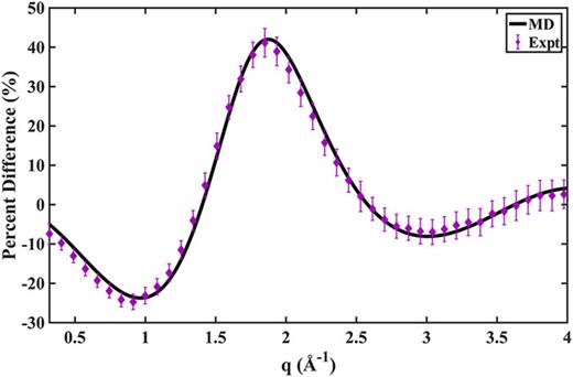
Percent difference scattering patterns of hot HT, for 100% excitation. Expt.: experimental results with error bars (given in 1σ),14 scaled by the 6.0% excitation fraction. MD: simulated hot scattering pattern from MD trajectories, averaged from the 2–3 ps interval of 150 trajectories.
Percent difference scattering patterns of hot HT, for 100% excitation. Expt.: experimental results with error bars (given in 1σ),14 scaled by the 6.0% excitation fraction. MD: simulated hot scattering pattern from MD trajectories, averaged from the 2–3 ps interval of 150 trajectories.
Distributions of structures of HT ensemble at high temperature
From the agreement of the scattering signals derived from the MD method with the experimental results, we conclude that the ensemble of molecular structures extracted from MD after convergence is reached represents the hot HT ensemble very well. We can therefore use the MD results to further study the distributions of structural parameters of hot HT, particularly all bonded interatomic distances and the farthest interatomic distance (see Fig. 11). Because of the rigidness of the chemical bonding, the distributions of bonded interatomic distances remain well characterized with a distinct maximum peak. However, for large nonbonded interatomic distances, the shapes of the distributions become complicated and not well-defined, as illustrated in Fig. 11(b). The distribution seems to have at least three peaks (around 3.6 Å, 4.8 Å, and 5.3 Å), indicating that it is indeed a hot ensemble of HT containing all three different conformers as well as various transition state structures. It is evident that it is implausible to use Eq. (2) and expect meaningful bond parameters to result.

Distributions of selected interatomic distances of hot HT modeled by MD trajectories used in calculating the pattern in Fig. 10. (a) Three bonded interatomic distances of HT as identified in the legend; dots are the original histograms and lines are interpolations for each histogram. (b) Histogram of the C1—C6 distance of the hot HT ensemble.
Distributions of selected interatomic distances of hot HT modeled by MD trajectories used in calculating the pattern in Fig. 10. (a) Three bonded interatomic distances of HT as identified in the legend; dots are the original histograms and lines are interpolations for each histogram. (b) Histogram of the C1—C6 distance of the hot HT ensemble.
Table II lists the distances of maximum probability of all bond distances of hot HT extracted from MD. For comparison, a set of experimental structural parameters determined previously from electron diffraction data by Ruan et al. are also listed.7 These latter distances were obtained by fitting the experimental scattering data using Eq. (2) with Rij and lh,ij being adjustable parameters. Although the fitted electron scattering curve matched well with their experimental data, the resulting fit parameters are questionable. As highlighted in bold, the fits gave 1.40 Å for the C2—C3 bond distance and a very large 1.71 Å bond distance for C4—C5. The distributions of HT structures from the MD ensemble give C2—C3 and C4—C5 values that are centered around 1.50 Å, even though here the energy distributed to the HT molecules is higher (200 nm photon). This disagreement emphasizes the importance of a careful treatment of the hot-molecule scattering pattern for the interpretation of the time-resolved X-ray and electron scattering data.
Bond distances and vibrational amplitudes of hot HT. Ref. 7: electron diffraction values by Ruan et al. Distance of maximum probability: the values where the distributions [Fig. 11(a)] have the largest probability.
| Bond distance (Å) | Reference 7 | Distance of maximum probability |
|---|---|---|
| C1=C2 | 1.29 | 1.334 |
| C2—C3 | 1.40 | 1.495 |
| C3=C4 | 1.41 | 1.355 |
| C4—C5 | 1.71 | 1.495 |
| C5=C6 | 1.32 | 1.333 |
| Bond distance (Å) | Reference 7 | Distance of maximum probability |
|---|---|---|
| C1=C2 | 1.29 | 1.334 |
| C2—C3 | 1.40 | 1.495 |
| C3=C4 | 1.41 | 1.355 |
| C4—C5 | 1.71 | 1.495 |
| C5=C6 | 1.32 | 1.333 |
CONCLUSION
In summary, a method for modeling scattering patterns of hot molecules using molecular dynamics simulations is introduced. The gas-phase 1,3-cyclohexadiene and its isomer 1,3,5-hexatriene (HT) at thermally hot conditions (∼2870 K) are used as examples. Excellent agreement between the hot scattering patterns calculated from the MD method and the experimentally measured X-ray scattering signals is obtained. Three important phenomena affect the scattering patterns: distance shifts, anharmonicity, and the correlation between internuclear distances. While the change in distances and the anharmonicity contributes prominently, the correlation between internuclear distances during the vibrational motions cannot be neglected.
It is noteworthy that although the examples in this paper are based on X-ray scattering, the concept is equally applicable to electron scattering. A set of unreasonable structural parameters determined previously from electron diffraction data might be related to the inappropriate use of the conventional analytical equations. Future investigations of pump-probe scattering data need to be mindful of the limitations of conventional approaches.
The structure of the transition state, on top of the barrier to interconversion between the CHD isomers, is found to contribute significantly to the scattering signal. Because the transition state has a very different structure than the equilibrium structure at the bottom of the double well potential, its difference signal is strong. Consequently, even though only a small fraction of the molecular ensemble is near the barrier at any given time, its contribution to the scattering signal of the hot system is important. It is possible that this finding could lead to novel methods to measure the structures of molecules at transition states. We anticipate that the present studies on modeling hot molecules provide an essential toolbox for exploring chemical reactions far from equilibrium and transition state structures using scattering techniques.
ACKNOWLEDGMENTS
This work was supported by the U.S. Department of Energy, Office of Science, Basic Energy Sciences, under Award DE-SC0017995, and by the Army Research Office (Grant No. W911NF-17-1-0256). A.K. acknowledges the Carnegie Trust for the Universities of Scotland under research Grant No. CRG050414 and the Royal Society of Edinburgh under Sabbatical Fellowship 58507. N.Z. acknowledges a Carnegie Ph.D. Scholarship from the University of Edinburgh. D.B. acknowledges an EPSRC Ph.D. Studentship from the University of Edinburgh. H.Y. acknowledges funding from the Brown University Global Mobility Research Fellowship and Brown University Doctoral Research Travel Grant for supporting research visits at the University of Edinburgh. Use of the Linac Coherent Light Source (LCLS), SLAC National Accelerator Laboratory, was supported by the U.S. Department of Energy, Office of Science, Office of Basic Energy Sciences under Contract No. DE-AC02-76SF00515.

