


Proteins within nanoporous hydrogels have important biotechnological applications in pharmaceutical purification, tissue engineering, water treatment, biosensors, and medical implants. Yet, oftentimes proteins that are functional in solution lose activity when in contact with soft, nanostructured, condensed phase materials due to perturbations in the folded state, conformation, diffusion, and adsorption dynamics of the protein by the material. Fluorescence microscopy experimentally measures the biophysical dynamics of proteins within hydrogels at the nanoscale and can overcome the limitations of conventional ensemble techniques. An explanation of the benefits of fluorescence is provided, and principles of fluorescence microscope instrumentation and analysis are discussed. Then several nanoscale fluorescence microscopies that image nanoscale protein dynamics within hydrogels are introduced. First, location-based super-resolution imaging resolves the adsorption kinetics of proteins to charged ligands within hydrogels used in pharmaceutical separations. Next, correlation-based super-resolution techniques image the heterogeneity of the nanoscale pore size of the hydrogels and the diffusion of analytes within the pores simultaneously. Finally, fluorescence resonance energy transfer imaging combined with temperature jump perturbations determines the folding and stability of a protein within hydrogels. A common finding with all three fluorescence microscopies is that heterogeneous nanoporous hydrogel materials cause variability of protein behavior dependent on gel sterics and/or interfacial electrostatic forces. Overall, in situ observations of proteins in hydrogels using fluorescence microscopies can inform and inspire soft nanomaterial design to improve the performance, shelf life, and cost of biomaterials.
I. UNDERSTANDING PROTEIN INTERACTIONS WITH HYDROGEL MATERIALS
Hydrogels are hydrophilic polymeric materials with high water content that have a nanoporous structure. Due to their hydrophilicity, hydrogels are typically biocompatible. This has led to diverse biotechnological uses of hydrogels. In medicine, hydrogels can be used for implants and plastic surgery1 and doping hydrogels with therapeutic proteins can be used for drug delivery.2 The similarity of synthetic hydrogels to the natural extracellular matrix extends their use as two- and three-dimensional cell culture matrices3 and in tissue engineering.4 Hydrogels can prevent erosion when used as a soil conditioner and can deliver protein nutrients to crops in the agricultural industry.5 Due to the sieving properties of their nanoporous structure, hydrogels are used to purify biologic therapeutics in the pharmaceutical industry.6 Biodegradable hydrogels are also being explored to be used as enzyme sensors and enzyme-sensitive drug delivery systems.7–9 In all of these applications, proteins come into contact with synthetic- or natural-hydrogel materials.
Understanding the biophysical function and dynamics of proteins in nanoporous hydrogels is challenging due to instrumental limitations. Most studies of protein folding and dynamics have focused on in vitro solution samples. Experimentally, samples must be cuvette-compatible and not scatter a significant amount of light for common spectroscopic methods that characterize proteins, such as circular dichroism, fluorometry, NMR, UV-vis, etc. Hydrogels present challenges in that they are a soft material that can scatter a significant amount of light. The nanoscale features of hydrogels also present heterogeneities that are averaged by common ensemble techniques which measure micro- to macroscale areas of the sample simultaneously. Therefore, more work needs to be done in developing methods to understanding proteins in hydrogel environments.
Fluorescence microscopy experimentally measures protein dynamics within hydrogels at the nanoscale and can overcome the limitations of conventional ensemble techniques. By labeling proteins with a fluorescent molecule, high signal to noise ratios (SNR) are achieved with commercially available instruments.10 Scattering from the hydrogel is reduced by strategic sample preparation and optical design to measure smaller axial sections of the sample. The influence of the micro- and nanoscale features of the hydrogel on protein dynamics is resolved by imaging on a microscope. Analysis of the resulting spatiotemporal signal by localization, correlation, and relative intensity accesses protein dynamics, including concentration, adsorption, diffusion, orientation, conformation, and folding.
Here, we explain the concepts of fluorescence microscopy, instrumentation, and analysis that are used to measure protein dynamics on the nanoscale within hydrogels in Sec. II. We then present three different experimental applications of fluorescence microscopies that quantify protein adsorption, diffusion, and folding within industrially- and medically-relevant hydrogels (Fig. 1). In Sec. III, super-resolution imaging of the adsorption kinetics of a fluorescently-labeled protein to charged ligands functionalized on a hydrogel surface determine the heterogeneity in protein separations important in the pharmaceutical field.6,11–13 In Sec. IV, correlative imaging of the diffusion of fluorescent emitters within the mesh of a hydrogel resolve both the nanoporous structure of the hydrogel and the diffusion dynamics of the emitters.14 In Sec. V, imaging the temperature-dependent fluorescence resonant energy transfer signal of proteins determines how hydrogel chemistry and confinement affects protein stability and folding kinetics.15 This tutorial illustrates that the design of hydrogel materials can then be informed by the molecular observations of the protein dynamics using these novel fluorescence spectroscopies, and future directions are discussed in Sec. VI.

Properties of protein dynamics in hydrogels that can be studied using fluorescence microscopy.
Properties of protein dynamics in hydrogels that can be studied using fluorescence microscopy.
II. WHY FLUORESCENCE?
A. Principles of fluorescence and sample considerations
Fluorescence is a luminescence process that allows for specific components in samples, such as proteins, to be detected with high signals in complex materials, such as hydrogels. In the simplest description of fluorescence, light is used to excite an electron from the ground electronic state to an excited state, as represented in the Jablonski diagram in Fig. 2(a). The molecule will be in an excited vibrational energy state within the excited electronic state and decay to the ground vibrational state through nonradiative processes. For fluorescence, the molecule will relax radiatively back to the ground electronic state, emitting a photon red-shifted from the excitation. The red-shift in fluorescence is critical to allow the emission to be separated from the excitation with spectral filters for detection [Fig. 2(b)]. Compared to alternative spectroscopic phenomena such as absorption, Raman, or Rayleigh scattering, fluorescence with appropriate high quantum yield fluorophores can achieve high signals (∼105 photons/s). Fluorescence is typically performed in the visible or near-visible range of the electromagnetic spectrum so practical instrumentation can be utilized.
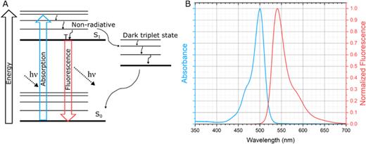
Energy and spectral representations of fluorescence. (a) The Jablonski diagram represents the basic energy principles behind fluorescence. The dark triplet state can cause fluorophores to temporarily go dark, or “blink,” which can be utilized for super-resolution techniques that require stochastic fluctuations. (b) Absorbance and emission spectra of fluorescein molecule in ethanol.16,17
Energy and spectral representations of fluorescence. (a) The Jablonski diagram represents the basic energy principles behind fluorescence. The dark triplet state can cause fluorophores to temporarily go dark, or “blink,” which can be utilized for super-resolution techniques that require stochastic fluctuations. (b) Absorbance and emission spectra of fluorescein molecule in ethanol.16,17
Proteins can be selectively detected in fluorescence microscopy by labeling the protein of interest with a fluorophore. The fluorophore can be a small conjugated organic molecule. Using high-affinity reactions with amine- (nitrogen-containing) or thiol- (sulfur-containing) chemistry, specific native- or mutated-amino acids within the protein can be labeled. Alternatively, fluorescent proteins, such as the thoroughly-studied green fluorescent protein (GFP), can be used. Fluorescent proteins can be directly attached to the protein in genetic expression within cells, which can be of benefit when studying proteins in biological hydrogels such as the extracellular matrix. A drawback of fluorescent proteins is that they are larger than their organic small molecule fluorophore counterparts (for example, the hydrodynamic radius, Rh ∼ 3 nm for GFP vs Rh ∼ 0.7 nm for rhodamine).18 Regardless of either type of fluorescent label, it is important to reduce the perturbations that the label has on the protein function based on the size, location, and charge of the label. Finally, the quantum yield and photostability of the fluorophore should be considered to ensure enough photons can be detected over the course of a measurement.
Hydrogel samples must be appropriately prepared for microscopy to detect fluorescently-labeled proteins within them. Hydrogels are typically obtained as a starting material in a powder or diluted liquid form. To create a hydrogel for some materials, such as agarose, the powdered agarose can be mixed in water, heated, and cooled to form a gel (Fig. 3). For other hydrogels, additional chemical cross-linking reagents may be required to create covalent- or ionic-bonds to form a gel, such as with polyacrylamide (covalent bisacrylamide) or alginate (ionic Ca+2). The hydrogel must be as free as possible from contamination, as Raman scattering or fluorescence from impurities, deemed “autofluorescence,” decreases the signal-to-background ratio of the protein signal. Without proper experimental design and controls, autofluorescence can even lead to false detection of contaminants instead of the actual protein. Light waves must also be able to pass through the hydrogel sample without interference due to scattering or absorbance.19 Hydrogel samples prepared with a lower percentage of polymer/cross-linker and more uniformity are preferred. Due to their high water content, hydrogels on the macroscale can be viewed as having similar refractive indices compared to water so that optical systems optimized for aqueous samples are compatible with hydrogel-based samples. But the variable densities of polymers within the hydrogel can lead to spatial fluctuations in the refractive index at the micro/nanoscale. Refractive index matching practices by adding biocompatible water-soluble agents can be used to reduce optical aberrations for hydrogels with more drastic differences between the polymer and surrounding solvent.20
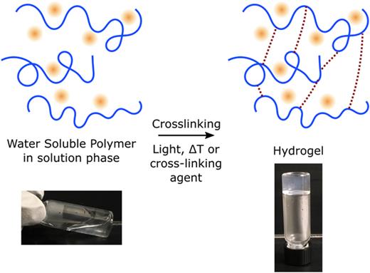
Synthesis of hydrogels by cross-linking of water-soluble polymers. Hydrogels are water-soluble polymer molecules (blue) that are cross-linked by applying either light, temperature change, or a cross-linking agent depending on the type of hydrogel. Fluorescent proteins or fluorophores (red) can be embedded in hydrogels as shown. Pictures show the creation of an agarose hydrogel by heating (soluble, left) and subsequently cooling (gel, right).
Synthesis of hydrogels by cross-linking of water-soluble polymers. Hydrogels are water-soluble polymer molecules (blue) that are cross-linked by applying either light, temperature change, or a cross-linking agent depending on the type of hydrogel. Fluorescent proteins or fluorophores (red) can be embedded in hydrogels as shown. Pictures show the creation of an agarose hydrogel by heating (soluble, left) and subsequently cooling (gel, right).
B. Fluorescence microscopy instrumentation
A fluorescence microscope is constructed to allow for excitation of the sample, separation of the emitted fluorescence from the excitation light, and detection of the fluorescence. Fluorescence microscopy has been around since its invention in the early 20th century.21 In order to image fluorescence emitted by a microscopic sample, it has to be excited by incident light, which is usually a single wavelength from a laser or a band of wavelengths from a band-filtered white light source [Fig. 4(a)]. The microscope should also be able to separate the red-shifted emitted light from the incident excitation, which is performed by the use of specifically designed filters [Fig. 4(b)]. A dichroic filter has a special thin film coating that reflects the excitation wavelength toward the objective lens. The coating transmits the red-shifted fluorescence emission collected by the objective lens, which is directed toward the detector. A traditional dichroic filter transmits redder wavelengths and hence is a long-pass filter, but there are other specialized dichroic filters that allow or reflect only a selected band of wavelengths that can be viewed as a combination of bandpass and long-pass filters. Efficient separation of the excitation laser light from the fluorescence is a required condition for obtaining high image contrast.
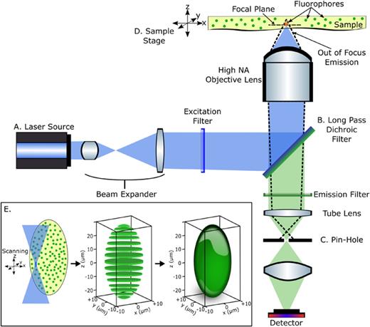
Schematic of an epifluorescence confocal microscope. (a) Blue or near blue excitation source which can be either a laser or a band-filtered white light source. (b) Dichroic long-pass filter to remove red-shifted fluorescence emission from excitation. The dotted lines show the fluorescence emission from out of focus areas which are being blocked by (c) the pinhole. (d) The sample stage can be moved across the focal point of the objective lens to collect 3D images. (e) An example depicting the generation of 3D image of a hydrogel bead captured by confocal scanning microscope as 2D sectioned images.
Schematic of an epifluorescence confocal microscope. (a) Blue or near blue excitation source which can be either a laser or a band-filtered white light source. (b) Dichroic long-pass filter to remove red-shifted fluorescence emission from excitation. The dotted lines show the fluorescence emission from out of focus areas which are being blocked by (c) the pinhole. (d) The sample stage can be moved across the focal point of the objective lens to collect 3D images. (e) An example depicting the generation of 3D image of a hydrogel bead captured by confocal scanning microscope as 2D sectioned images.
Fluorescence microscopes are described by the different configurations between the excitation and detection paths, different ways to focus and collect light from the sample, and detectors used. We will focus on a standard reflection microscope configuration where the excitation and the detection of light are passed through the same objective equipped with optical components that allow for the separation of excitation and emission spectra, which is known as an epifluorescence microscope.
1. Confocal microscopy
Confocal microscopy improves the resolution of fluorescence microscopy by removing out of focus light with a pinhole.22 An epifluorescence microscope has a similar optical resolution as a standard optical microscope as the light emitted from outside the focus regions are collected by the imaging optics. In an effort to increase the resolution, the confocal microscope was developed to remove out of focus light by the use of a simple pinhole that increases resolution tremendously.23 The basic components of a confocal microscope are shown in Fig. 4. The out of focus light from outside the focal plane (dotted rays) are blocked by the cleverly-placed pinhole in front of the detector [Fig. 4(c)].
The resolution of a confocal microscope is largely dependent on the objective lens and diffraction limit of the light. The spot size of illumination by an objective lens is given by the radius of the first Airy disk24–26
Here, rAiry is the Airy pattern radius from the central peak to the first minimum, λ is the wavelength of the excitation light, and NA is the numerical aperture of the objective lens. The diameter of the first Airy disc is defined as the Airy Unit (AU). The lateral image resolution is defined by Eq. (2), and the axial resolution is defined by Eq. (3). Here, n is the refractive index of the immersion medium. It can be seen from these equations that the resolution is inversely proportional to the numerical aperture of the objective lens. Thus, a large numerical aperture objective lens is required to obtain fine resolutions of the order of hundreds of nanometers,
The size of the pinhole to use depends on parameters of the objective lens and governs the resolution and SNR of the captured images. A pinhole of 1AU diameter provides the best SNR. A pinhole that is smaller than 1AU diameter will improve the resolution provided the fluorescence signal is strong. For a confocal microscope system that uses 532 nm excitation and a 100×, 1.4 NA objective lens to image, the diameter of the Airy disc, as per Eq. (1), would be 464 nm. Since the pinhole is placed on the image plane of the objective lens, this diameter will have to be multiplied by the magnification of the objective lens. Thus, the pinhole size for best SNR for this system should be 46.4 μm. However, in most practical imaging systems, a pinhole of the order of 100 μm is used that compromises SNR to ease of optical alignment and maintenance.
A confocal microscope is capable of collecting 3D image data because of the improved resolution. Images on a confocal microscope are not directly captured but are rendered by scanning either the objective lens or the sample stage scans through the x/y plane and along the z-axis [Fig. 4(d)]. The data are collected on a one-dimensional detector, which is a high efficiency detector like an avalanche photodiode or a photomultiplier tube. The collected data are processed to produce 2D and 3D images based on the known location of the sample with respect to the collection time [Fig. 4(e)]. Since this is not a direct image capture method like epifluorescence or reflective optical microscopy, special attention needs to be paid toward image size defined in number of pixels. Following Nyquist sampling rules, the pixel size should be smaller than the lateral resolution divided by 2.3.27
The confocal microscope was a huge development in terms of resolution from a standard fluorescence microscope but was still restricted in resolution because of the diffraction limit. In 1873, Ernst Abbe defined the diffraction limit of light to be
where d is the minimum resolvable distance when the observation is being made by a light of wavelength λ and a lens of numerical aperture NA. The lateral and the axial resolutions of a confocal microscope are given by Eqs. (2) and (3). For the same confocal microscope system that uses 532 nm excitation and a 100×, 1.4 NA objective lens to image, the calculated lateral resolution is 190 nm, while the axial resolution is 400 nm. It has been demonstrated experimentally that the resolution of fluorescence microscopy techniques is restricted to ∼200 nm laterally and ∼500 nm axially.22,28–30 However, this is still much larger than the size of proteins or small fluorescent molecules. The axial resolution in a confocal microscope is much larger than the lateral resolution, because of the diffraction of light by a lens.
2. Total internal reflection fluorescence microscopy
The axial resolution of the focal volume is reduced to <100 nm in Total Internal Reflection Fluorescence Microscopy (TIRFM) by using a very simple technique of total internal reflection at an interface.31 TIRFM exploits the unique properties of an induced evanescent wave or field in a limited specimen region immediately adjacent to the interface between two media having different refractive indices. TIRFM utilizes total internal reflection at the interface of the glass coverslip and aqueous-based hydrogel sample. As per Snell's law of refraction, this will happen if the angle of incidence is larger than the critical angle. This critical angle depends on the refractive index of the two media and is governed by the following expression:
Here, θc is the angle of incidence and n2 and n1 are the refractive indices of the two media. A necessary condition for total internal reflection to occur is n2 < n1. In the schematic example shown in Fig. 4, refractive indices of an aqueous medium (1.3) and glass coverslip (1.5) are appropriate to support the total internal reflection at the interface. When the laser excitation incident angle is larger than the critical angle of 62°, the beam is reflected back into the objective lens at the glass and aqueous medium interface. This results in the generation of an evanescent field adjacent to the interface. The intensity of the electromagnetic field that is dissipated along the axial (z) direction at the interface can be represented as32
where d is the depth of penetration of the evanescent field. Depth of penetration depends only on the two refractive indices, the wavelength of light used, and the angle of incidence and is usually a few hundreds of nanometers. The excitation efficiency decreases exponentially with the distance from the interface as mentioned in Eq. (6). In this way, TIRFM is able to achieve much higher axial resolution. The type of TIRFM illumination that is shown in Fig. 5 is known as objective-based TIRFM. This requires NA of the objective lens to be extremely high (>1.3). TIRFM illumination can also be achieved by placing a prism over the sample for excitation and collecting the emission by an objective underneath the sample. This kind of microscopy where the angle of incidence of illumination is increased with the help of a prism is known as prism-based TIRFM.31
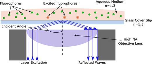
Concept of Total Internal Reflection Fluorescence Microscopy (TIRFM). Excitation region in the sample is restricted to the interface of the glass cover slip and the aqueous medium by total internal reflection.
Concept of Total Internal Reflection Fluorescence Microscopy (TIRFM). Excitation region in the sample is restricted to the interface of the glass cover slip and the aqueous medium by total internal reflection.
TIRFM can be used to detect individual molecules on the sample surface provided the fluorophores that are used have high fluorescence quantum yield and are present in low concentrations. Signals emitted by such high resolution techniques are of the order of a few hundred thousand photons. So, 2D, highly light-sensitive detectors (EMCCD or sCMOS) that have low noise, 100 Hz frame rates, up to 95% quantum efficiency, 6–10 μm pixel size for 60×–100× magnification, and large fields of view (18–25 mm) are required for capturing fluorescence signals.
C. Fluorescence microscopy analysis
Analysis of spatiotemporal data obtained by confocal microscopy and TIRFM with localization, correlation, and relative intensity can be used to quantify protein dynamics, including concentration, adsorption, diffusion, orientation, conformation, and folding. This section provides an overview of different analyses based on localizing single molecules, correlating the signal for the detection of many single molecules, or analyzing the behavior of micromolar concentrations of fluorescently-labeled molecules. This only serves as a brief introduction to these techniques and the reader should refer to cited articles dedicated to each of the individual methods for more detailed information.
1. Super-resolution imaging by single molecule localization
In order to visualize molecules beyond the diffraction limit, a family of super-resolution analysis techniques has been developed based on localization.33 While known by many different acronyms, Photoactivated Localization Microscopy (PALM),34 Stochastic Optical Resolution Microscopy (STORM),35 and Points Accumulation for Imaging Nanoscale Topography (PAINT)36 are some of the more commonly used methods. These techniques temporally isolate fluorescence signal from a single fluorophore within the ensemble and localize the centroid of an individual molecule to subdiffraction-limited spots. A super-resolved image can then be generated using the data from the individually localized single fluorophores that break the diffraction limit of light. Figure 6 illustrates the steps to produce a super-resolution image by localization. Diffraction-limited spots (∼250 nm for green light) of individual molecules are isolated [Fig. 6(a)] so that the centers are localized with a precision of ∼10s of nm by fitting the spot to a two-dimensional Gaussian or related point spread function model [Fig. 6(b)]; a statistical buildup of the locations of multiple single molecule events [Fig. 6(c)] leads to an image below the diffraction limit [Fig. 6(d)].
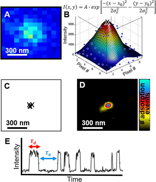
Super-resolution imaging and kinetics of protein adsorption to ligands in hydrogels. (a)–(d) Steps to produce a super-resolution image of ligand locations from multiple protein adsorption events. (a) The diffraction-limited emission pattern of a fluorescently-labeled protein adsorbed to a ligand. (b) Fitting the raw data of the point spread function (blue points) to a two-dimensional Gaussian (surface; mathematical fitting equation written above) obtains the centroid location (black “x”). (c) Centroids from multiple, stochastic adsorption events localize the ligand within the hydrogel to ∼30 nm, as shown in (d), the final super-resolution image. (e) Kinetic information is obtained by monitoring the intensity at an individual ligand location versus time. Increase in intensity indicates an adsorbed protein.
Super-resolution imaging and kinetics of protein adsorption to ligands in hydrogels. (a)–(d) Steps to produce a super-resolution image of ligand locations from multiple protein adsorption events. (a) The diffraction-limited emission pattern of a fluorescently-labeled protein adsorbed to a ligand. (b) Fitting the raw data of the point spread function (blue points) to a two-dimensional Gaussian (surface; mathematical fitting equation written above) obtains the centroid location (black “x”). (c) Centroids from multiple, stochastic adsorption events localize the ligand within the hydrogel to ∼30 nm, as shown in (d), the final super-resolution image. (e) Kinetic information is obtained by monitoring the intensity at an individual ligand location versus time. Increase in intensity indicates an adsorbed protein.
Localization-based super-resolution imaging utilizes signal from isolated single molecules. But is worth noting that not all single molecule techniques obtain subdiffraction-limited super-resolutions (see Secs. II C 2–II C 5) and not all super-resolution techniques use single molecules (see Sec. II C 4). There are also many other techniques that are used to improve the resolution of the fluorescence microscopy like Stimulated Emission Depletion (STED)37 and Ground State Depletion (GSD),38 etc., that use the nonlinear response of fluorophores to light excitation. A detailed discussion of all the different localization techniques is beyond the scope of this tutorial.
2. Single molecule adsorption kinetics
Fluorescence localization microscopy can also provide information on how frequently adsorption or reaction events take place over time, i.e., kinetic information, in addition to where events take place with spatial localization. Protein adsorption kinetics at individual super-resolved binding sites in hydrogels can be calculated by counting the number and length of events from frame-to-frame to obtain the desorption time (i.e., dwell time of an individual molecule) and adsorption time (i.e., the waiting time between one molecule leaving and a new molecule adsorbing to the same site) [Fig. 6(e)]. Cumulative distributions of all of the desorption and adsorption times can quantify the deviation from monoexponential kinetics and the degree of heterogeneity.
3. Correlation analysis of diffusion
Correlation analysis can provide diffusion and spatial information from fluorescence signals. Correlation is an objective signal processing technique that measures the self-similarity of a signal over time. In the form of fluorescence correlation spectroscopy (FCS), the diffusion constant of molecules can be calculated.39–41 In FCS, a stationary diffraction-limited focal volume on a confocal microscope is focused within a hydrogel and fluorescently-labeled molecules diffuse through the focal volume. Their emitted signal is collected on a one-dimensional detector and the resulting fluorescence intensity vs time signal is detected, F(t). The fluctuations in the signal, δF(t) are calculated by
which are then analyzed by autocorrelation
where G(τ) is the normalized autocorrelation function given by the overlay of the original function with its shifted self at a given lag time τ. The resulting autocorrelation function decays over time and can be fit to a model derived from the Stokes-Einstein relationship for three-dimensional diffusion and the focal volume size
where Veff is the effective volume, ⟨C⟩ is the average concentration of fluorescent molecules, τd is the diffusion time, and rxy and rz are the lateral and axial beam radii. The diffusion time is related to the translational Brownian diffusion coefficient, D, by
With FCS, and its imaging analogs,42,43 diffusion coefficient information can be obtained at diffraction-limited resolutions.
4. Super-resolution imaging by correlation
Correlation analysis produces super-resolution images in super-resolution optical fluctuation imaging (SOFI),44 which correlates the signal from spatially-fixed, stochastically blinking fluorophores (dark state, Fig. 2).44–47 A desired structure of interest is labeled with fluorescent molecules that blink (turn on and off). Blinking is a stochastic process for each of the independent fluorophores. The fluorophores are typically imaged on a wide field or TIRFM setup and detected on a two-dimensional detector over time. The signal F(t) at each pixel located at location, r, and frame time, t, is given by
where U(r) is the diffraction-limited emission pattern of the individual fluorophore, ε is the brightness of the fluorophore, and s(t) is the probability that the fluorophore is either on (=1) or off (=0). U(r) is called the point spread function and can be approximated by a three-dimensional Gaussian
where x, y, and z are the center location of the molecule and the ω0 and ωz0 are the lateral and axial width of the Gaussian pattern, respectively. Similar to FCS, the fluctuations in the signal at each pixel are analyzed by autocorrelation over lag times, τ,
The resulting U(r)2 reduces the width of the emission pattern to ω0,new = ω0/. Plotting the autocorrelation amplitude for each pixel results in an image below the diffraction limit of ∼100s of nanometers, although resolution improvements by a factor of 10 have been demonstrated with higher order correlations.48,49
5. Förster resonance energy transfer (FRET) analysis of protein folding
Förster (or Fluorescence) Resonance Energy Transfer (FRET) can obtain <10 nm distance information by observing the nonlinear response of emission from two fluorophores to the excitation of light.50,51 In FRET, the proximity between two dye molecules is determined by using the principle of nonradiative energy transfer between a donor and an acceptor molecule. The ratio of donor-to-acceptor fluorescence (D/A) is very sensitive to nanoscale changes in distance. The FRET efficiency (E) is the quantum yield of the energy transfer. It varies as the inverse sixth power of the donor-to-acceptor separation (r)
where R0 is the Förster distance for this donor-acceptor pair. It is highly efficient when this separation is less than the Förster radius, which is the distance at which D/A is half (typically 3–6 nm). Thus, FRET can provide accurate measurements of molecular separation down to angstrom distances (10–100 Å).50 Since this length scale is similar to the size of many proteins, FRET is often used to understand protein folding and conformational changes by placing the two dyes at strategic locations on a protein and analyzing the D/A either for an ensemble of proteins or a single molecule.
Labeling strategies and appropriate analysis controls must be carefully considered when applying FRET to proteins.52,53 Donor-acceptor pairs with Förster distance ranges of 2.2–8.5 nm are commercially available in the forms of either genetically incorporated fluorescent proteins or organic fluorophores for site-selective labeling (Sec. II A).52 Selected donor and acceptor locations should be positioned for optimal sensitivity to anticipated known motions and unfolding distances of the proteins and should not interfere with protein function. Furthermore, the labels should have a controlled or predictable orientation to reduce the uncertainties in donor–acceptor distance.54,55 Appropriate analysis controls must be designed to determine that each protein is labeled with one donor and one acceptor (and not two donors or two acceptors) and that neither the donor or acceptor is photobleached. Typically, in single molecule FRET experiments this is confirmed by observing anticorrelated emission intensities from separate donor and acceptor channels.51
III. SUPER-RESOLUTION IMAGING OF PROTEIN ADSORPTION IN HYDROGELS
A. Use of hydrogels for pharmaceutical separations
Now that we have established a foundation in fluorescence microscopy principles in Sec. II, we can now consider what medical- and industry-relevant problems pertaining proteins in hydrogels we can apply these powerful techniques to. Chromatography is an important analytical technique used in a variety of industries (petrochemical, food product, environmental analysis, pharmaceutical) to separate molecules based on size, charge, hydrophobicity, chirality, or specific affinities. Specifically, as the pharmaceutical industry has shifted to using biologics—proteins, peptides, and nucleic acids—as therapeutic molecules, the optimization of chromatography has grown to be a time- and cost-intensive step in the research, development, and production of drugs. This is compared to the historically more common small-molecule drugs which could be more easily isolated through strategic synthetic methods. Separating mixtures of biologics can account for 50% of the $2.6 billion dollar average cost in bringing a drug to market.56
Hydrogels are often used as stationary phase support in chromatography due to their high surface area-to-volume ratios and the ability to modify the gel surface chemistry. The nanoporosity of a hydrogel can be tuned by varying the amount of monomer and cross-linker used when polymerizing the gel. The surface chemistry of the hydrogel can be controlled by chemically conjugating specific ligands to the gel surface. Hydrogel-based chromatography is performed by flowing an analyte protein within a mixture of molecules in an aqueous liquid mobile phase over the hydrogel stationary phase support. The analyte interacts through noncovalent interactions with the hydrogel. These could include steric separation based on the size of the analyte compared to the nanoporous mesh of the hydrogel and packing of individual microscale hydrogel beads or electrostatic/hydrophobic/specific affinity separation based on interactions of analyte with the chemistry of the hydrogel surface. The differences in the number and length of the interactions for different molecules with the hydrogel lead to their separation over time.
Single molecule fluorescence microscopy can help avoid costly, empirical, iterative optimization of conditions used in hydrogel separations by providing mechanistic information on chromatography that is hidden in ensemble measurements. Difficult separations that have skewed, non-Gaussian, overlapping peaks arise from multiple populations of analyte dynamics. Single molecule spectroscopy resolves individual events that correlate to the different Gaussian subpopulations that underlie the broad or asymmetric peaks, revealing the causes from a mechanistic perspective not possible through traditional techniques.
B. Application—Analysis of protein adsorption in hydrogels at super-resolution length scales reveals that the sterics of the hydrogel pores cause heterogeneity in protein purification
Single molecule super-resolution imaging resolved heterogeneity in nanoporous agarose hydrogels relevant to biologic ion-exchange separations. Ion-exchange chromatography separates molecules based on the electrostatic affinity of a charged analyte to specific ionic functional groups in the hydrogel. In multiple works by Kisley and Landes,11–13,57 an agarose hydrogel was modified with cationically-charged peptide ligands (polymers of agininamide) to separate an anionic analyte (the protein α-lactalbumin). The protein was labeled with a single Alexa555 fluorophore at the N-terminus for imaging.
Fluorescence imaging can be used to super-resolve single protein binding events at single ligands in chromatography [Figs. 6(a)–6(d)]. By utilizing low concentrations and the timescale of the adsorption kinetics of the protein to the ligands, super-resolution imaging of the ligand locations is achieved using a form of PAINT.36,58 When the protein was not adsorbed to the hydrogel, the diffusion of the protein was too fast compared to the temporal resolution of the detector and the signal was “blurred out.” Analysis was then carried out by the localization and kinetic procedure described in Fig. 6 and Secs. II C 1 and II C 2. Results on the spatial charge-distribution of ligands,11,57 the reduction of kinetic heterogeneity by ionic strength,12 and the blocking of ligands by competing proteins13 have been observed in hydrogels with single molecule techniques.6
A common finding throughout multiple studies was that the sterics of the nanoporous agarose hydrogel stationary phase support cause separation heterogeneity (Fig. 7). The adsorption kinetics of proteins at individual ligands followed an expected monoexponential behavior [insets, Fig. 7(a)], indicating a stochastic adsorption process was occurring. However, between different ligands, the adsorption rates varied by over an order of magnitude. Studies increasing the weight percent of agarose from 1% to 3%, which in turn decreased the nanoporosity of the hydrogel, decreased the number of binding events with long adsorption times [Fig. 7(b)], and decreased the total number of binding events [Fig. 7(b)]. Therefore, the amount of hydrogel present tunes the degree of heterogeneity present in the separation.

The sterics of the nanoporous hydrogel cause separation heterogeneity. Adsorption site heterogeneity can be reduced by increasing agarose content. (a) Cumulative distributions of the adsorption times of proteins binding events to all of the ligands observed in a 160 μm2 area over 5 min. The ensemble heterogeneity is reduced as agarose content is increased. Dashed lines provided as a guide for the eye. (a, inset) Adsorption times are homogeneous at individual ligands in 1% agarose. Solid lines are fits of the data to monoexponential kinetic models. (b) Increasing agarose content reduces the total number of adsorption events. (c) Time course of confocal laser scanning microscopy images of the distribution of thyroglobulin (red) in an agarose-based chromatography particle. Diffusion of the protein is restricted toward the surface of the particle based on steric restrictions. Figures are adapted with permission from Kisley et al., Proc. Natl. Acad. Sci. U.S.A. 111, 2075–2080 (2014). Copyright 2014 National Academy of Sciences11 and Matlschweiger et al., J. Chromatogr. A 1585, 121–130 (2019). Copyright Elsevier, 2018.59
The sterics of the nanoporous hydrogel cause separation heterogeneity. Adsorption site heterogeneity can be reduced by increasing agarose content. (a) Cumulative distributions of the adsorption times of proteins binding events to all of the ligands observed in a 160 μm2 area over 5 min. The ensemble heterogeneity is reduced as agarose content is increased. Dashed lines provided as a guide for the eye. (a, inset) Adsorption times are homogeneous at individual ligands in 1% agarose. Solid lines are fits of the data to monoexponential kinetic models. (b) Increasing agarose content reduces the total number of adsorption events. (c) Time course of confocal laser scanning microscopy images of the distribution of thyroglobulin (red) in an agarose-based chromatography particle. Diffusion of the protein is restricted toward the surface of the particle based on steric restrictions. Figures are adapted with permission from Kisley et al., Proc. Natl. Acad. Sci. U.S.A. 111, 2075–2080 (2014). Copyright 2014 National Academy of Sciences11 and Matlschweiger et al., J. Chromatogr. A 1585, 121–130 (2019). Copyright Elsevier, 2018.59
Imaging at the hydrogel particle-scale with confocal microscopy has complemented molecular scale imaging to understand protein adsorption in chromatography. Developed by Ljunglöf and Hjorth60 and used routinely by other groups such as Carta et al.59,61 and Lenhoff et al.,62 confocal laser scanning microscopy has imaged the distribution of proteins within micrometer-scale hydrogel particles to quantify protein adsorption affinity [Fig. 7(c)]. Complexities in protein adsorption kinetics and uptake have been revealed to be related to the larger proteins being sterically-limited to interacting within only the first few micrometers of the particle, bound protein layers hindering the diffusion of smaller proteins,59 and nondiffusive electrokinetic contributions to protein transport.62
Overall, these results support that the steric obstacles within the nanopores of the hydrogel are a source of heterogeneity in separations. This is consistent with why hydrogel-based chromatography supports sometimes use a “spacer arm” between the ligand and the hydrogel matrix63 to avoid steric effects. Characterization of the distribution, not just the average, porosity of hydrogels would further the understanding of how hydrogel sterics influence protein separations.
IV. CORRELATION ANALYSIS IMAGES THE NANOSCALE PORE DISTRIBUTION AND QUANTIFIES DIFFUSION WITHIN HYDROGEL MATERIALS
A. Correlation signal processing can image hydrogels in situ compared to other conventional microscopy techniques
Given the influence of the nanoporous mesh size of the hydrogel on protein separations, is there a way we can image the nanoporous agarose material itself? Can we understand how the nanopores affect the diffusion of the proteins?
Current techniques that image hydrogel porosity have drawbacks in perturbing the sample or producing averaged values. Electron microscopy can image hydrogel pores but requires the gel to be flash frozen in liquid nitrogen to maintain the structure within the vacuum sample chamber. Given the high water content of hydrogels, this perturbs the native structure. Electron microscopy also can only image the surface of the hydrogel unless sectioning of the gel is performed, which can further disrupt the hydrogel structure. Similarly, scanning probe methods such as atomic force microscopy (AFM) can be used but are also limited to the surface structure of the hydrogel. AFM also has challenges when high scanning forces are needed to image the soft and deformable surface of the hydrogel. X-ray diffraction and other scattering techniques are ensemble techniques that obtain average pore sizes but do not provide spatially-resolved information about the pores. There is, therefore, a need for a characterization technique that provides in situ characterization of the relationship between heterogeneous nanoscale structure of the hydrogel and a functional property such as diffusion or adsorption.
We were motivated to use the benefits of correlation analysis from both FCS and SOFI discussed in Secs. II C 3 and II C 4 to obtain simultaneous super-resolution and diffusion information in nanoporous hydrogel materials. In our technique, fcsSOFI, fluorescent emitters are able to diffuse within the nanopores of the hydrogel and imaged on a two-dimensional camera (Fig. 8). The fluctuations in signal arise from the diffusion of the emitters [Fig. 8(a)]. In the resulting movie, pixels where the pores are located have emitters and fluctuations in intensity [Fig. 8(b)]. Emitters are unable to access areas where the polymeric hydrogel is present and appear dark with no intensity fluctuations beyond the detector noise. Correlation analysis is applied to each pixel vs time [Fig. 8(c)]. The resulting autocorrelation curve vs time lag has both spatial and diffusion information. For the super-resolution spatial SOFI portion, the amplitude of the correlation curve at the first time lag is plotted as the image saturation (how bright the image is). With the addition of an image deconvolution step, a super-resolution image is produced that outperforms the diffraction limit by approximately a factor of two, similar to Eq. (13). For the diffusion FCS portion, the autocorrelation curves at each pixel are fit to an empirical model of diffusion to obtain the diffusion coefficient, similar to Eqs. (9) and (10). The resulting calculated diffusion coefficient is plotted on the image as the hue or color. A final image fusion step combining the SOFI saturation and FCS hue produces the final fcsSOFI super-resolution image of the hydrogel nanopores and the emitter diffusion within them [Fig. 8(d)]. fcsSOFI can, therefore, produce nanoscale images of the interior of hydrogels in situ without requiring the drawbacks of freezing, high forces or averaging that are required with current techniques.
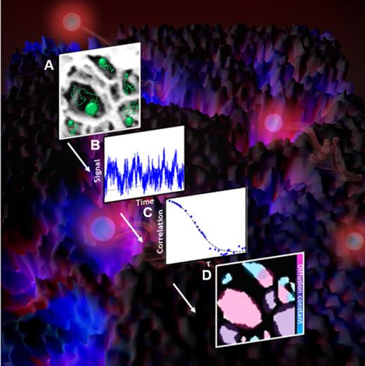
Steps of fcsSOFI analysis. (a and background image) Fluctuations in signal are produced by fluorescent emitters diffusing within the nanopores of the hydrogel. (b) The fluctuations in intensity at each individual pixel over time are analyzed by (c) autocorrelation. The amplitude of the autocorrelation curve is plotted as the saturation of the image and curve fitting to a diffusion model is plotted as the color of the (d) final fcsSOFI image. Adapted with permission from Kisley et al., ACS Nano 9, 9158–9166 (2015). Copyright 2015 American Chemical Society.14
Steps of fcsSOFI analysis. (a and background image) Fluctuations in signal are produced by fluorescent emitters diffusing within the nanopores of the hydrogel. (b) The fluctuations in intensity at each individual pixel over time are analyzed by (c) autocorrelation. The amplitude of the autocorrelation curve is plotted as the saturation of the image and curve fitting to a diffusion model is plotted as the color of the (d) final fcsSOFI image. Adapted with permission from Kisley et al., ACS Nano 9, 9158–9166 (2015). Copyright 2015 American Chemical Society.14
B. Application—The heterogeneous porosity and diffusion within agarose hydrogels
fcsSOFI applied to agarose hydrogels qualitatively shows the varied distribution of nano- and micro-sized pores and inaccessible parts of the hydrogel (Fig. 9). Agarose hydrogels were prepared at 1% (w/w) with 100 nm fluorescent bead emitters within them. The traditional diffraction-limited average images [Fig. 9(a)] compared to the resulting fcsSOFI images [Fig. 9(b)] show the sensitivity of correlation to weak fluctuations due to the 150-fold improvement in the signal-to-background contrast. Focusing on the fcsSOFI images [Fig. 9(b)], the dark areas of the image are the locations of hydrogel inaccessible to the fluorescent emitters, while the bright areas show heterogeneous pore sizes with heterogeneous diffusion present.
![FIG. 9. fcsSOFI analysis of pore size and diffusion within an agarose hydrogel. (a) Average diffraction-limited image in 1% agarose. No features are incorrectly observed in the 1% agarose due to the low excitation power used resulting in a low signal-to-background ratio (<2). (b) Super-resolution diffusion map obtained by fcsSOFI shows heterogeneous diffusion [highlighted by arrows; purple, log(D/nm2/s) ∼ 4; red, log(D/nm2/s) ∼ 6] of average log(D/nm2/s) = 4.8 ± 0.8 in 1% agarose. (c) Quantitative super-resolved agarose pore sizes. Scale bars are all 1 μm. Adapted with permission from Kisley et al., ACS Nano 9, 9158–9166 (2015). Copyright 2015 American Chemical Society.14](https://aipp.silverchair-cdn.com/aipp/content_public/journal/jap/126/8/10.1063_1.5110299/4/m_081101_1_f9.jpeg?Expires=1716322930&Signature=QSDLcAQ0dcqjdEGriuoELXgzgoKkDdE9gb4ZLJ6mpQvezs3reiqi1eQaWjnPxfg6hNUXlXRguI5crvyk3isaZmDCRpxaExW6rIIzmzaeJ5SyRbWdJu0BiNDATqyVfTxdTzei08c7-b2nH9hg2QF0j-OIFgMfbL2rDMfjOyXqNvpgoUmQbQkWvd7jN7IXbE~8mEZ4l3hbe6AwsreryzmoRjuqO6UQuMQnqjRA~SXQCBVf9MbYRmmrbKUKLlv7e-7~mI44OXzoIBXTCOTvJsDehQ8OJ286JmsASpPr~HuyU~pdNfMSwM~ughQHgrRq3Q5f8otcLzr9C3hTvj6hLR4iQw__&Key-Pair-Id=APKAIE5G5CRDK6RD3PGA)
fcsSOFI analysis of pore size and diffusion within an agarose hydrogel. (a) Average diffraction-limited image in 1% agarose. No features are incorrectly observed in the 1% agarose due to the low excitation power used resulting in a low signal-to-background ratio (<2). (b) Super-resolution diffusion map obtained by fcsSOFI shows heterogeneous diffusion [highlighted by arrows; purple, log(D/nm2/s) ∼ 4; red, log(D/nm2/s) ∼ 6] of average log(D/nm2/s) = 4.8 ± 0.8 in 1% agarose. (c) Quantitative super-resolved agarose pore sizes. Scale bars are all 1 μm. Adapted with permission from Kisley et al., ACS Nano 9, 9158–9166 (2015). Copyright 2015 American Chemical Society.14
fcsSOFI analysis of pore size and diffusion within an agarose hydrogel. (a) Average diffraction-limited image in 1% agarose. No features are incorrectly observed in the 1% agarose due to the low excitation power used resulting in a low signal-to-background ratio (<2). (b) Super-resolution diffusion map obtained by fcsSOFI shows heterogeneous diffusion [highlighted by arrows; purple, log(D/nm2/s) ∼ 4; red, log(D/nm2/s) ∼ 6] of average log(D/nm2/s) = 4.8 ± 0.8 in 1% agarose. (c) Quantitative super-resolved agarose pore sizes. Scale bars are all 1 μm. Adapted with permission from Kisley et al., ACS Nano 9, 9158–9166 (2015). Copyright 2015 American Chemical Society.14
Quantitative assessment of the pore size distribution showed a bimodal population of pores within the 1% agarose [Fig. 9(c)]. Two populations of 240 ± 40 nm and 1000 ± 500 nm are observed. The normal distribution with heterogeneity, 240 ± 40 nm, agrees with previous reports; the outliers, 1000 ± 500 nm, are unexpected and may be due to the connectivity of multiple pores and the two-dimensional projection of a three-dimensional volume in the image. In the quantitative analysis of the diffusion constants obtained by correlation analysis, an average of log(D/nm2/s) = 4.8 ± 0.8 is obtained in the 1% hydrogel. More interestingly, correlation analysis shows the spatial heterogeneity of diffusion coefficients at super-resolution levels [arrows, Fig. 9(b)]. Smaller diffusion coefficients could arise from increased confinement within the agarose, where diffusion becomes anomalous and the Brownian fitting model is no longer appropriate. Future work correlating the pore sizes to diffusion dynamics is needed, along with expanding the technique to the diffusion of fluorescent proteins within the hydrogels.
fcsSOFI offers a visual representation of both diffusion and pore size that can complement prior studies of diffusion within hydrogels measured by FCS on confocal microscopes. FCS analysis of polymeric macromolecules in silica nanostructures,64 polyacrylamide,65 and dextran66 hydrogels and single particle tracking of quantum dots in polyacrylamide hydrogels67 are some examples of prior measurements that have quantified non-Brownian diffusion within nanoporous materials.68 Yet, these techniques lack a visual map of pore locations. Future work incorporating anomalous diffusion models or maximum entropy methods64,69 into fcsSOFI will advance the technique to quantify more diverse dynamics of protein diffusion in hydrogels.
V. FAST RELAXATION IMAGING (FReI) SHOWS HYDROGEL CHEMISTRY AFFECTS PROTEIN FOLDING MORE THAN CONFINEMENT IN NANOPORES
As the prior discussed microscopies demonstrated that protein adsorption and diffusion are affected by the nanoporous nature of hydrogels, we then asked: Does the nanoporous confining nature of hydrogels affect the folding, conformation, and stability of proteins? The stability of a protein is sensitive to its surrounding environment. When proteins interact with a material such as a hydrogel, the local microenvironment of the gel can cause perturbations in the protein energy landscape (Fig. 10). The energy landscape defines the folding pathways, final folded state, and activity of the protein.71 Therefore, a hydrogel can alter the structure and conformational dynamics and hence, function of a protein compared to when the protein is in solution and in vivo.72,73

Perturbation of the energy landscape of a protein upon interacting with a hydrogel. Cartoon of free energy landscapes and dye-labeled structure of the protein phosphoglycerate kinase (PGK)70 in solution vs within a hydrogel. Changes in protein structure (location of the global energy minimum), stability (magnitude of energy minimum), and folding rates (steepness, barriers, and local energy minima) can be described by the two landscapes (red, blue). These properties can be measured by FReI through the donor-to-acceptor ratio in fluorescence (D/A; green-to-red), which increases as the protein goes from native folded (left) to perturbed unfolded (right) forms.
Perturbation of the energy landscape of a protein upon interacting with a hydrogel. Cartoon of free energy landscapes and dye-labeled structure of the protein phosphoglycerate kinase (PGK)70 in solution vs within a hydrogel. Changes in protein structure (location of the global energy minimum), stability (magnitude of energy minimum), and folding rates (steepness, barriers, and local energy minima) can be described by the two landscapes (red, blue). These properties can be measured by FReI through the donor-to-acceptor ratio in fluorescence (D/A; green-to-red), which increases as the protein goes from native folded (left) to perturbed unfolded (right) forms.
A. Protein folding can be imaged using fluorescence resonance energy transfer and temperature jumps
Protein folding dynamics can be characterized in hydrogels using Fast Relaxation Imaging (FReI).15 FReI was initially developed to study protein folding in vivo within cells.74 FReI uses proteins labeled with a FRET pair. In FReI, a series of temperature jumps are applied as a function of time. The temperature jumps are step-shaped increases of 4–6 °C that equilibrate within milliseconds of the initial jump and have an 8 s dwell time. By monitoring D/A before, during, and after the temperature change, the initial state, unfolding, and refolding of the protein can be spatiotemporally monitored. The D/A ratio increases as the donor moves further away from the acceptor as the protein unfolds. Decreases in D/A after protein unfolding at high temperatures indicate intermolecular FRET due to aggregation. By monitoring the D/A vs the equilibrated temperatures for all jumps, the protein folding thermodynamics is quantified [Fig. 11(a)]. Analyzing the D-A vs time for an individual temperature jump follows the folding kinetics of the protein [Fig. 11(b)]. Finally, pixel-by-pixel analysis shows how the protein how heterogeneous the protein stability is as a function of position within the gel.
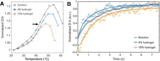
Hydrogel chemistry affects protein folding more than confinement within the nanopores. FReI measurements of (a) equilibrium thermodynamics and (b) folding kinetics of PGK-FRET in solution, in 4% polyacrylamide, and in 10% polyacrylamide. Adapted with permission from Kisley et al., ACS Appl. Mater. Interfaces 9, 21606–21617 (2017). Copyright 2017 American Chemical Society.15
Hydrogel chemistry affects protein folding more than confinement within the nanopores. FReI measurements of (a) equilibrium thermodynamics and (b) folding kinetics of PGK-FRET in solution, in 4% polyacrylamide, and in 10% polyacrylamide. Adapted with permission from Kisley et al., ACS Appl. Mater. Interfaces 9, 21606–21617 (2017). Copyright 2017 American Chemical Society.15
B. Application—Comparison of hydrogel surface chemistry and nanoporous confinement effects on protein folding
The effect of both hydrogel surface chemistry and nanoporous confinement on protein folding was assessed by preparing polyacrylamide hydrogels at two different conditions. At a 4% (w/w) preparation, polyacrylamide has larger pores and minimal confinement that it is statistically similar to the protein in solution.75 Alternatively, a 10% (w/w) preparation of polyacrylamide has significant confinement effects within the nanopores, being four times smaller than those in the 4% hydrogel. By comparing protein folding in solution and in the 4% hydrogel to the 10% hydrogel, the effect of confinement is tested. Comparing the solution results to both the 4% and 10% hydrogel results tests the effect of the chemistry of the hydrogel. The enzyme phosphoglycerate kinase (PGK) that has been studied extensively in vivo and in vitro in solution76,77 was chosen as a model protein. PGK is an important enzyme in glycolysis, functioning as a catalyst during the transfer of a phosphate group to ADP to produce ATP. Therefore, understanding the folding of PGK will relate to its enzymatic function. PGK was modified with mCherry (acceptor) and AcGFP1 (donor) fluorescent proteins fused at the C- and N-termini, respectively, for the FRET pair.
Thermodynamic analysis of FReI data shows that the protein is stabilized in the 4% nonconfining hydrogel but aggregates more easily upon unfolding in both hydrogels. The sigmoidal shape of the thermodynamic plot of the normalized D/A vs temperature shows the protein going from a folded to unfolded state [Fig. 11(a)]. The inflection point of the sigmoidal curve is the melting temperature (Tm) of the protein and indicates the thermodynamic stability. The turnover in the sigmoidal curves after the melting temperature indicates the protein aggregation temperature [Fig. 11(a), dashed lines]. The melting temperature qualitatively shifts to a higher temperature in both the hydrogels compared to in solution [Fig. 11(a), arrow]. More pronounced is that the protein aggregates at a lower temperature in hydrogels once it unfolds (Taggregate = 58 ± 3 °C in solution to Taggregate = 51 ± 2 °C in the 10% hydrogel).
Kinetic analysis of FReI data shows that protein folding speeds up and is more heterogeneous in the hydrogels compared to in solution. The normalized donor minus acceptor fluorescence at the melting temperature was analyzed vs time with a stretched exponential model [Fig. 11(b)]. Statistically identical folding rates of 1.2 ± 0.3 s and 1.3 ± 0.5 s were found in the 4% and 10% hydrogels, respectively, compared to 2.2 ± 0.2 s in solution. The stretching factor, which falls between 0 and 1, where 1 is for monodisperse homogeneous folding, was 1 in solution, but decreased to ∼0.9 in both hydrogels.
Overall, the presence of the hydrogel chemistry, i.e., electrostatic forces at the hydrogel surface, was shown to be more important than any confinement effects of the nanopores. The fact that the thermodynamic and kinetic data show similar behavior of the protein in the 4% and 10% hydrogels compared to that in solution highlight that the chemical presence of hydrogel has the most effect on the protein. We speculate that possible destabilizing interactions between the hydrogel and protein could be due to energetically-favorable amide-amide hydrogen bonding78,79 that cause the unfolded protein to aggregate to the gel. Further work varying the amide content of the hydrogel through hydrolysis or copolymer hydrogels could further support this. We also analyzed the imaging results of the FReI data but saw the folded state of the protein was homogeneous at the 500 nm pixel size of microscope. Additional development of super-resolution imaging combined with FReI could resolve heterogeneity at the length scale of the pores within the hydrogel.
VI. SUMMARY
The development and use of fluorescence microscopies have revealed important effects of the nanoporous heterogeneity and surface chemistry of hydrogels on protein dynamics. Fluorescence microscopies can be used at concentration regimes from single molecules (PAINT), pseudosingle molecule nanomolar concentrations (fcsSOFI correlates the signal from many single emitter events) to ensemble micromolar concentrations (FReI). A common finding with all three microscopies was that heterogeneous nanoporous materials cause variability of protein behavior. This is in contrast to the commonly-held assumption that proteins maintain the same dynamics in hydrogels as in solution due to the high water content of hydrogels. What we have observed is that this is not the case in studies with different hydrogels (agarose, polyacrylamide) and different proteins (α-lactalbumin, PGK).
Beyond the discussed protein/hydrogel samples, PAINT, fcsSOFI, and FReI can be applied to additional biomolecule-material interactions such as polymer brush surfaces,68,80,81 “antifouling” polymers,82–84 homogeneous and patterned surfaces,85,86 nucleic acids,87–89 the protein corona around therapeutic nanoparticles,90–93 and protein-ligand complexes.94–97 Further, these fluorescence microscopies are not just limited to samples with a biological component. Fluorescence microscopies that have been developed for cellular imaging have much untapped potential to be applied to materials science. Solid-state materials such as quantum,98 catalytic,99,100 and plasmonic47,101–104 nanomaterials and porous zeolites105 have been studied with super-resolution microscopies. Condensed matter physicists should consider exploring the fluorescence microscopy resources in nearby medical and biology departments and how these powerful techniques could be applied to address the bio/nano/polymeric material questions they have.
While this tutorial has focused on experimental approaches to protein/hydrogel interactions, developing theoretical methods to further understand experimental results is an interesting area of biophysics that needs more development. In terms of theoretical modeling of protein folding and dynamics, many force fields approximate solvents and are computationally expensive when water and salts are added explicitly into atomistic simulations, slowing simulations down by orders of magnitude.106 Theoretical modeling polymer dynamics is an entirely separate field itself with its own distinct set of force fields for atomistic and coarse-grained models.107 Incorporating both proteins and polymers into modeling with force fields that can appropriately model both is a lofty future challenge that will require a concerted effort of many scientists.
ACKNOWLEDGMENTS
We thank the Case Western Reserve University College of Arts and Sciences for financial support. The Arnold O. and Mabel M. Beckman Foundation provided additional support during the early writing of this manuscript through the Beckman-Brown Interdisciplinary Postdoctoral Fellowship. Additional thanks to Professor LaShanda Korley for kindly nominating us for a tutorial in the Journal of Applied Physics.
NOMENCLATURE
- AFM
Atomic force microscopy
- AU
Airy unit
- FCS
Fluorescence correlation spectroscopy
- FReI
Fast relaxation imaging
- FRET
Förster resonance energy transfer
- GFP
Green fluorescent protein
- NA
Numerical aperture
- PAINT
Points accumulation for imaging nanoscale topography
- PGK
Phosphoglycerate kinase
- TIRFM
Total internal reflection fluorescence microscopy
- SNR
Signal to noise ratio
- SOFI
Super-resolution optical fluctuation imaging

