

The truth of history is no simple matter, all packed and parcelled ready for handling in the market-place.
Herbert Butterfield (Reference Butterfield1931: 132)
In social science history, the Big Book of 2014 was surely Thomas Piketty's Capital in the Twenty-First Century.Footnote 1 It was big in bulk (685 pages). More significantly, it was big in its impact. Piketty's book is about the concentration of wealth and the dynamics of economic inequality. It relies on two centuries of historical data from 20 countries. The book attracted a good deal of attention for its scope and breadth and for its bold and startling predictions, the most disturbing of which is the following:
It is almost inevitable that inherited wealth will dominate wealth amassed from a lifetime's labor by a wide margin, and the concentration of [wealth] will attain extremely high levels—levels potentially incompatible with the meritocratic values and principles of social justice fundamental to modern democratic societies. (Piketty Reference Piketty2014a: 26)
By the time the English translation of the book appeared in April 2014, the distribution of wealth in the United States was already the object of public discussion and concern. Inequality had been front-page news during the Occupy Wall Street encampments in Zuccotti Park in the fall of 2011. Those protests focused on the disparity between those in the top 1 percent of the wealth distribution and those in the bottom 99 percent.Footnote 2 Coming at the right time, Piketty's book, with its frightening prediction, hit a nerve and injected new frisson into both the scholarly and the partisan debates.Footnote 3 Prominent economists were quick and effusive with their praise. Robert Solow called it a “new and powerful contribution” (Reference Solow2014). Paul Krugman called the book “magnificent” (Reference Krugman2014c), “the most important economics book of the year—and maybe of the decade” (Reference Krugman2014a), and noteworthy because, unlike many trade books on economic issues, it constitutes “serious, discourse-changing scholarship” (Reference Krugman2014b). Branko Milanovic writing in the Journal of Economic Literature described it as a “watershed book in economic thinking” (Reference Milanovic2014: 519).
Most commenters agreed that an unqualified strength of the book was its quantitative history. Alexander Field's review essay in the Journal of Economic History praised the book as “both an exemplary work in quantitative economic history and economic literature in the finest sense” (Field Reference Field2014: 916). Krugman cited its “unmatched historical depth” (Reference Krugman2014c). Lawrence Summers declared: “Even if none of Piketty's theories stands up, the establishment of (the historical facts) . . . is a Nobel Prize-worthy contribution” (Reference Summers2014). Peter Lindert, writing for a French audience, claimed the book, with its “solid empirics,” has “transported us to a higher understanding of historical movements in inequality.”Footnote 4
Piketty covered a wide range of historical statistics. He documented the long period trends in the top income and wealth shares for the last two centuries. He estimated time series for the top 10 percent and the top 1 percent of the two distributions. He reported data from the United States, France, the United Kingdom, Sweden, and Germany. The breadth of his coverage is daunting. Here, I narrow the focus. I report my efforts to describe the data, methods, and assumptions required to replicate Piketty's estimates for the top 1 percent of the wealth distribution for the United States. As Piketty notes, the underlying American data are less solid than those of the European countries, at least for the years before 1962, and are particularly shaky for the nineteenth century. Thus, it appears the American experience could claim a higher priority for reevaluation.
Piketty's estimates of American income inequality are limited to the twentieth century, but his wealth estimates begin in 1810. He and his commenters make much of the comparison of recent wealth estimates with those from the nineteenth century. Piketty refers repeatedly to the American Gilded Age as a period marked by extreme wealth inequality, created and intensified by end-of-life bequests (Piketty Reference Piketty2014: 348–350, 375, 377–78, 506).Footnote 5 “In all likelihood,” he predicted, “inheritance will again play a significant role in the twenty-first century, comparable to its role in the [nineteenth century]” (p. 377). Krugman titled his review of Piketty's book Why We're in a New Gilded Age and suggested the country is headed “back to ‘patrimonial capitalism,’ in which the commanding heights of the economy are controlled not by talented individuals but by family dynasties” (Reference Krugman2014c). Social science historians certainly have a stake in the question of whether we are in or headed into a “New Gilded Age.” They also have something to say about wealth accumulation in the original Gilded Age. One place to start, I suggest, is to review Piketty's quantitative estimates of wealth holdings. Can they be replicated?
Academics, journal editors, and the federal agencies funding scientific and social scientific research have recently become concerned about the difficulty sometimes encountered in assessing the reliability of reported findings. Reports on how frequently researchers in cell biology and social psychology (to name just two examples) failed to reproduce published results have become well known both within those fields and throughout the larger community (Bohannon Reference Bohannon2015; Buck Reference Buck2015). And rightly so. The inability to reproduce key findings undermines the credibility of the scientific enterprise. Science, a publication of the American Association for the Advancement of Science, “the world's leading journal of original scientific research,” convened a forum on the problem of reproducibility and issued a set of recommendations for promoting an open research culture (Nosek et al. Reference Nosek, Alter, Banks, Borsboom, Bowman, Breckler, Buck, Chambers, Chin, Christensen, Contestabile, Dafoe, Eich, Freese, Glennerster, Goroff, Green, Hesse, Humphreys, Ishiyama, Karlan, Kraut, Lupia, Mabry, Madon, Malhotra, Mayo-Wilson, McNutt, Miguel, Paluck, Simonsohn, Soderberg, Spellman, Turitto, VandenBos, Vazire, Wagenmakers, Wilson and Yarkoni2015). A specific suggestion for scientific journals was to encourage and incentivize attempts to replicate significant findings. Piketty's discourse-changing effort certainly qualifies as significant.
The panel also emphasized a researcher's obligation to make their data and methodology transparent and open. On this score Thomas Piketty earns high marks. His practice is far better than most. He has made his data available and has documented his methodologies in a set of online technical appendixes, spreadsheets, and supplemental commentary. Had he not done so, this replication exercise would not have been possible. Still, the replication was not easy; Piketty's documentation was not always complete and his guidance was sometimes difficult to follow.
Estimates for the Twentieth Century, the Top 1 Percent
Piketty used two basic sources to estimate the distribution of wealth in the twentieth century and up to 2010 (Piketty Reference Piketty2014: 347). One is the archive of estate tax returns filed with the Internal Revenue Service and analyzed by Wojciech Kopczuk and Emmanuel Saez (Reference Kopczuk and Saez2004). The modern estate tax was introduced in 1916 and has remained part of the tax code ever since (Luckey Reference Luckey2011). These records provide information on the wealth at death of those with estates that exceed the exemption level. Kopczuk and Saez employed a technique known as the “estate multiplier” to convert the data on wealth of the deceased into an estimate of the percentage of wealth going to the top 1 percent of the living population annually from 1916 through 1950, from 1982 through the year 2000, and for 10 separate years between 1951 and 1981 (Kopczuk and Saez Reference Kopczuk and Saez2004: table 3, 454–55). Their method requires the age and sex of each decedent, information that is also recorded in the tax records. With this methodology each estate tax return is weighted by the inverse probability of death at that age. This means the wealth of individuals who die young—a rare event—is given a higher weight reflecting the fact that the estate tax records contain relatively fewer observations of wealth at those ages.Footnote 6
Piketty's second source is the periodic Survey of Consumer Finances (SCF) conducted by the Flow of Funds unit of the Federal Reserve. These surveys include an oversampling of the very rich and have been conducted irregularly in the years 1962, 1969, 1983, 1989, 1992, 1995, 1998, 2001, 2004, 2007, 2009, 2010, and 2013. The SCF has been analyzed in a series of studies by Edward Wolff who summarized his results in two recent articles (Wolff Reference Wolff2013, Reference Wolff2014). The SCF data have also been independently used to produce estimates for the top 1 percent for the years spanning 1989 through 2009 by Flow of Funds staff researchers (Bricker et al. Reference Bricker, Bucks, Kennickell, Mach, Moore, Hulten and Reinsdorf2015; Kennickell Reference Kennickell2009, Reference Kennickell2012).
Both data sets are imperfect as a measure of the concentration of wealth (Kopczuk Reference Kopczuk2015); but one important point to note is the estate tax returns reflect the wealth of individuals while the SCF covers spending units. Spending units are defined to include all individuals living in a household and this definition implicitly assumes they pool their resources. The relationship between the two measures can be seen in figure 1. The broken line for the period 1916 to 2008 is the measure estimated for individuals from the estate data.Footnote 7 The observations indicated by the solid dots are those reported by Wolff for 1962, 1969, and 1983–2013 for households (Wolff Reference Wolff2013 [2012: table 2, 50]; Reference Wolff2014: table 2, 50). The alternative SCF household series reported by the Federal Reserve is plotted with the solid line for 1989 through 2009 (Kennickell Reference Kennickell2009: table 4, 35; Reference Kennickell2012: note to table 5, footnote 12).Footnote 8
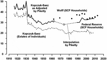
FIGURE 1. Percent of wealth owned by the top 1 percent of households. Picketty's adjustments of the estate data.
Piketty gives the impression the difference between the individual-level and the household-level measures is explained by the fact that a household measure “always leads to higher inequality” than if it was measured for individuals (Piketty Reference Piketty2014b: 56). The difference between the two measures is ambiguous because the size and sign of the gap depends upon the distribution of wealth within the family (Kopczuk and Saez Reference Kopczuk and Saez2004: 476). If the entire gap between the two measures in figure 1 is attributable to the distinction between individual and family measures, it would imply many wealthy families split their wealth between husband and wife.Footnote 9
The raw numbers presented in figure 1 were the “bedrock” employed by Piketty to produce the chart he published as figure 10.5 and reproduced here as figure 2 (Piketty Reference Piketty2014a: 348; Reference Piketty2014b: 1). To arrive at the smooth version he presented, Piketty made several adjustments to the data. Because he felt the SCF data is more reliable than the estate data he adjusted the Kopczuk-Saez series upward to link with the SCF data. For the years 1930 through 1960 he inflated the estimates of Kopczuk-Saez by a factor of 1.25 to obtain an estimate comparable to the SCF series. The spreadsheet that generated the data (TS10.1DetailsUS) suggests Piketty was influenced in this choice by the inflation factor required to bring the solid line up to reach his adjusted SCF estimate for 1962. For the years 1916 through 1929, Piketty used a multiplier 1.2, not 1.25, to move from the estate data to an estimate for the wealth share at the family household level. There is no explanation for the jump from 1.2 to 1.25 in 1930. The stability of the inflation factor, however, is dubious. Piketty implicitly assumed splitting household wealth between husband and wife was as common in the early decades of the twentieth century as it was in 1962. Separate estates, however, were infrequent in the early twentieth century before the spread of the community property ethic that regards the relationship between husband and wife as an economic partnership (Newcombe Reference Newcombe2011).
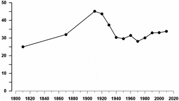
FIGURE 2. Percent of wealth owned by the top 1 percent of households (Picketty's figure 10.5).
Piketty then switched from the adjusted estate data to the SCF data at the earliest possible date, 1962. Kopczuk and Saez warn in this context that “patching together data from different sources is a perilous exercise” (Reference Kopczuk and Saez2004: 479). However, characteristic of his bold approach to the topic, Piketty did exactly that in a process he described as “homogenization” (Piketty Reference Piketty2014b: 56–58). The solid line for 1916–1960 at the left of figure 1 is simply the upward adjustment of the estate data. The first available data point based on the SCF is for 1962. The wealthiest 1 percent of the wealth distribution held 33.4 percent of total wealth that year (Wolff Reference Wolff2014: table 2, 50). Without explanation Piketty adjusted this downward to 31.4 by subtracting 2 percentage points. The adjusted number is represented by the open circle plotted for 1962 in figure 1. Chris Giles, a reporter for the Financial Times, described this procedure as “seemingly arbitrary” (Giles Reference Giles2014).Footnote 10 In a follow-up response to Giles, Piketty failed to explain the adjustment (Piketty Reference Piketty2014c). Because there were no surveys taken in the 1970s, Piketty simply inserted an arbitrary value for 1974 apparently designed to lie close to an extension of the inflated Kopczuk-Saez data. That number, 28.2 percent, is marked with the second open circle.Footnote 11 He then interpolated a straight line across the 15 years between the value for 1974 and the Federal Reserve's observation for 1989. Thereafter he followed the Federal Reserve's data through 2009.Footnote 12
The final step and an unfortunate one in Piketty's effort to chart the twentieth-century trend for the 1 percenters’ share of wealth was to smooth the raw data by plotting only decadal averages (see figure 2). The value plotted for 1920, for example, is the average of the adjusted Kopczuk-Saez data for the 1920s. However, only the decades for the 1920s, 1930s, and the 1940s have an observation for all 10 years. The data for 1910 is the average for 1916–19. The decades of the 1960s, 1980s, and 2010s are represented by a single observation each (1962, 1989, and 2007). Given the noise in the underlying data, some data smoothing is certainly reasonable. The smoothing also obscures the dramatic spike in inequality that occurred during the last half of the 1920s, which reached an all-time high in 1930 of more than 50 percent.Footnote 13 Smoothing over an entire decade makes it difficult to connect public policy changes, stock market swings, and other developments to changes in the distribution of wealth.
Estimates for the Nineteenth Century, the Top 1 Percent
Piketty admits in the “Technical Appendix” to his book that “huge uncertainties exist” on his nineteenth-century estimates (Piketty Reference Piketty2014b: 58). For the United States in the mid-nineteenth century, Piketty has only one real data point, an estimate for 1870. This is based on the census of wealth conducted at the time of the 1870 Census of Population (US Census Office 1870). Piketty cites the source for the 1870 observation as Lee Soltow (Reference Soltow1975: table 4.2, 99) as reported by Peter Lindert (Reference Lindert, Atkinson and Bourguignon2000: table 3, 188). Soltow's findings were based on an idiosyncratic “spin sample” drawn from the physical microfilms of the census enumerations. Soltow marked a spot on the glass screen of the microfilm reader, turned the crank a half turn, and sampled the individual whose name fell on the marked spot provided it identified a male 20 years old or older (Soltow Reference Soltow1975: 4–5). He proceeded in this fashion through all 1,761 rolls of microfilm for the 1870 Census!
Soltow's estimate of the total assets (the sum of personal assets and real estate) held by the top 1 percent of adult men in 1870 is 27 percent.Footnote 14 Piketty inflated Soltow's value to 32 percent presumably to convert total assets owned by the top individuals to net worth owned by the top households. Piketty offered no justification for this adjustment. He simply multiplied the 27 by 1.2, which is the same multiplier he used to make a similar conversion on the estate-derived data for 1916–29. That multiplier, however, was tenuously based on the comparison of Kopczuk and Saez's estimates for individuals in 1962 with Wolff's estimate for households notwithstanding the 98-year separation between the two dates, the different nature of the two sources (census reports vs. estate tax returns), and the implication that social and legal practices regarding the distribution of ownership within the family remained constant. Wives very rarely reported wealth separately from their husbands in the mid-nineteenth century. Under the common law of coverture wives could not legally be property owners.
If we take Piketty's value of 32 percent for 1870 at face value, it implies the share of wealth owned by the top 1 percent of households increased dramatically to reach 45.1 percent in 1910 (see figure 2). Piketty described the increasing concentration of wealth as an already “well-established fact” (Piketty Reference Piketty2014: 347).Footnote 15 It is unclear if this portrayal of the growth in inequality during the Gilded Age should be regarded as Piketty's quantitative measure of changes in the concentration of wealth or whether the manipulations performed on Soltow's numbers were intended to simply illustrate what was already widely believed by economic historians.
Piketty also plots a point in his figure 10.5 for 1810 (see figure 2). It is 25 percent suggesting there was an increasing concentration of wealth between 1810 and 1870. Piketty cited “Shamas [sic] Reference Shammas1993 and Lindert Reference Lindert, Atkinson and Bourguignon2000” as his sources (Piketty spreadsheet TS10.1). But neither Carole Shammas nor Lindert give a figure for 1810. Piketty started with Alice Hanson Jones's estimate for 1774 for all households, 16.5 percent, which is found in Lindert (Reference Lindert, Atkinson and Bourguignon2000: table 3, 188).Footnote 16 He rounded this to 17 percent and redated it to 1770. Piketty then turned his attention to Soltow's 1860 data for total assets owned by free adult males, 29 percent. To obtain an estimate for net worth of a household he applied the ubiquitous 1.2 adjustment multiplier. He then read a number for 1810 off a straight-line interpolation between 1770 and 1860, 24.9, and rounded it to 25 percent.
I can appreciate Piketty's desire to have a wealth concentration estimate for 1810, but I find his simple interpolation difficult to accept. Between 1774 and 1810 there was the Revolutionary War, which saw the departure of many wealthy United Empire Loyalists and a postwar period of mercantile and shipping prosperity during which some large fortunes were amassed in Philadelphia, Baltimore, New York, and Boston. Jefferson's Embargo of 1807 and the recession in 1809 hit these fortunes especially hard. I find it difficult to credit a straight-line interpolation through this turbulent period. Piketty has no persuasive evidence about what changes occurred in the distribution of wealth during the antebellum period. Thirty-four years before Piketty's book appeared, Jeffery Williamson and Peter Lindert suggested a “working hypothesis” that “wealth concentration rose over most of the period 1774–1860, with especially steep increases from the 1820s to the late 1840s” (Williamson and Lindert Reference Williamson and Lindert1980: 46). This hypothesis has held up according to more recent studies (Lindert Reference Lindert, Atkinson and Bourguignon2000: 190; Lindert and Williamson Reference Lindert and Williamson2013; Steckel and Moehling Reference Steckel and Moehling2001).
Estimates for the Top 10 Percent
The first point to make is that Piketty thinks the trend for the top 10 percent is a better indicator of inequality than the trend for the top 1 percent. At least in a recent issue of Science, Piketty has a coauthored review with Emmanuel Saez that presents the trend for the top 10 percent of households but not the companion series for the top 1 percent. The chart in Science reproduces the data from Piketty's book except the point for 1810 is missing, but now the chart inexplicably adds a point for 1890 that isn't in the book (Piketty Reference Piketty2014: figure 10.6; Piketty and Saez Reference Piketty and Saez2014: figure 2, 839). That added point is derived from a linear interpolation between 1870 and 1910. Figure 3 displays the diagram as it appears in Science.
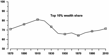
FIGURE 3. “Wealth Inequality in the United States, 1870-201” (Piketty-Saez in Science [Reference Piketty and Saez2014: figure 2]).
After examining Piketty's derivation of the long-period trend for the top 10 percent, I find it difficult to be forgiving. For 1870, Piketty reports Soltow's number taken from Lindert, 71 percent, but without applying a multiplier to convert individual-level data to the household level. Consistency suggests he should have made an adjustment or explain why one is not needed. Had he used the 1.2 multiplier applied to the data for the 1 percent, the 1870 figure would be 85.2 percent. But accepting that figure would compel Piketty to claim the concentration of wealth fell between 1870 and 1910. So much for the “well-established” fact that inequality was increasing during this period.
Piketty has no other evidence on the 10 percenters before 1980. As noted by Chris Giles, all the data plotted for 1910 through 1950 and for 1970 was obtained by simply adding 36 points to the data for the top 1 percent wealth share. The 36-point adjustment is not explained. The constancy of this markup, however, is questionable, particularly as one goes further back in time. The gap between the top 10 percent and the top 1 percent wealth shares reported for 1870 by Soltow, for example, was 43 percentage points, not 36 (Soltow Reference Soltow1975: table 4.2, 99).
The data point for 1960 was calculated by adding 35.6 points, not 36, to the 1 percent share, again without explanation, but strangely the 35.6-point adjustment is expressed as “33.6+2.”Footnote 17 For 1980 Piketty reported he averaged the 1983 figure from Wolff (Reference Wolff and Gonzalez2011) with the 1989 Federal Reserve figure from Kennickell (Reference Kennickell2009). Had he done that, the number would be 67.7, but he reported 67.2 (which is the 1989 figure).Footnote 18 For 1990 Piketty added 35.8, not 36, to get 68.7. This adjustment was also presented without explanation and in this case expressed as (36.9+34.7)/2.Footnote 19 For 2010 he claimed to be using an average of 2007 and 2009, but he reported only the number for 2007 because he had no data for 2009 (Bricker et al. Reference Bricker, Bucks, Kennickell, Mach, Moore, Hulten and Reinsdorf2015).
The caption to the figure in Science states the numbers are constructed from inheritance tax records, but that is only true for the data 1910–50. This cavalier handling of the data and his sources on the top 10 percent may not be a fatal flaw, but it is certainly unfortunate. It raises doubts about the care Piketty has taken with his evidence. It gives partisan critics an excuse to ignore his concerns and policy proposals.
Assessment of Piketty's Wealth Share Estimates
Very little of value can be salvaged from Piketty's treatment of data from the nineteenth century. The user is provided with no reliable information on the antebellum trends in the wealth share and is even left uncertain about the trend for the top 10 percent during the Gilded Age (1870–1916). This is noteworthy because Piketty spends the bulk of his attention devoted to America discussing the nineteenth-century trends (Piketty Reference Piketty2014: 347–50).
The heavily manipulated twentieth-century data for the top 1 percent share, the lack of empirical support for the top 10 percent share, the lack of clarity about the procedures used to harmonize and average the data, the insufficient documentation, and the spreadsheet errors are more than annoying. Together they create a misleading picture of the dynamics of wealth inequality. They obliterate the intradecade movements essential to an understanding of the impact of political and financial-market shocks on inequality. Piketty's estimates offer no help to those who wish to understand the impact of inequality on “the way economic, social, and political actors view what is just and what is not” (Piketty Reference Piketty2014: 20). It might be suggested Piketty's interest is in broad trends and does not extend in these directions, but his introduction to the book suggests these finer-grained economic, social, and political issues are salient and his book's conclusion offers policy suggestions that would require political action and some public consensus about what is just and what is not.
It is now possible to make a direct assessment of the twentieth-century history of inequality depicted by Piketty. Figure 4 compares the adjusted raw data he used to undergird his portrayal of the trend in the concentration of wealth with annual data subsequently published by Emmanuel Saez and Gabriel Zucman. Their series is calculated by capitalizing income flows reported in personal income tax returns (Saez and Zucman Reference Saez and Zucman2016). This alternative series was not available to Piketty when he drafted his book, but it has several advantages over the data he used. It is a direct, rather than an inferred, measure of household inequality and it is available annually for the crucial 1960–89 period, through which Piketty was forced to interpolate.
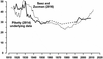
FIGURE 4. Percent of wealth owned by the top 1 percent of households.
From a policy perspective, several deficiencies in Piketty's underlying data stand out. Both series indicate that the Roaring Twenties saw an increase in inequality and that the Great Depression and the New Deal produced a reversal. This said, it is also true that the estimates of Saez and Zucman suggest that the twenties saw a particularly dramatic increase in concentration, which might be attributed to the reduction in the progressivity of the federal income tax following World War I. The reversal in inequality during the thirties and early forties according to Saez and Zucman was more gradual than Piketty's underlying data indicate. The postwar era through 1960, both series agree, was one of relative stability with the top 1 percent holding about 30 percent of the nation's wealth. However, the two series display important differences for the last half-century, 1960–2010, clearly the most relevant period for those concerned about the future direction of inequality trends.
The combination of homogenization and interpolation hides the continuing move toward equality between 1972 and 1982 and then neglects to reflect the rapid rebound toward concentration that took place between 1982 and the late 1980s. Piketty's underlying data for the 1990s and the first decade of the twenty-first century present yet another problem. With the Saez-Zucman series, the top wealth share has increased steadily since the mid-1980s to reach a postwar high of 41.8 percent by 2012. Piketty's series shows a modest increase in inequality over the decade of the 1980s and only a negligible change between 1990 and 2010. The last year of Piketty's series was 2009 with a wealth share of 33.8. Ironically, the new series is more consistent with Piketty's claim that equality “suffered a setback after 1980” than his own series (Piketty Reference Piketty2014: 350).
An Alternative Picture
It would be unfair to fault Piketty for failing to use data sources not available at the time he drafted Capital. Yet, thanks to the recent work by Saez and Zucman, it is now possible to avoid estimating the distribution of wealth across households by manipulating the estate tax data on individuals. Because Saez and Zucman provide estimates up to 2012 there is no need to link tax data with observations from the SCF. Because the income tax was introduced in 1913 and the estate tax in 1917, the Saez-Zucman series includes four additional years in the 1910s. Moreover, the capitalized income method they employ is clearly superior to the estate tax method of Kopczuk and Saez. The capitalized income approach does not employ a constant estate multiplier, does not require a constant mortality gradient by wealth, and is not subject to distortions produced by tax avoidance actions taken in anticipation of death (Saez and Zucman Reference Saez and Zucman2016: 524, 570–72).
There is also no need to rely on Soltow's limited report on wealth in 1870 because the Integrated Public-Use Microdata Project at the University of Minnesota (IPUMS) has made available a 1 percent random sample of the house-by-house returns originally recorded by the census enumerators (Rosenbloom and Stutes Reference Rosenbloom, Stutes and Rosenbloom2008; Ruggles et al. Reference Ruggles, Alexander, Genadek, Goeken, Schroeder and Sobek2010a). Piketty is correct to insist that household-level data is superior to individual-level data. Fortunately, it is possible to use the IPUMS sample to generate household-level data comparable to the twentieth-century data generated from income tax returns by Saez and Zucman. In a data appendix, I discuss the nature and reliability of the 1870 Census of wealth data. I conclude that the IPUMS sample can provide an adequately reliable picture of the top wealth shares in the United States in that year.
The top panel of table 1 presents the wealth shares in 1870 calculated for the top 1 percent and the top 10 percent of households. In the full sample, there are more than 75,000 households. The top 1 percent held 27.8 percent of the nation's wealth, somewhat less than the 32 percent suggested by Piketty. The IPUMS sample can also be used to examine wealth at the level of the individual adult. My calculations of the individual wealth shares include all adults 18 and over. These estimates, reported in the middle panel of the table, put the top 1 percent for all adults at 39.8 percent. Soltow's spin sample included only adult males. When only males are included in the calculations based on the IPUMS sample, the top 1 percent share drops to 28.5 percent (or 30.9 percent for males 20 and older, comparable to the 27 percent reported by Soltow).
TABLE 1. Top wealth shares, United States, 1870
Source of estimates in bold: Author's calculations based on the IPUMS sample of the US Census of 1870.
Of particular interest, however, is that in 1870 the wealth share at the individual level is considerably higher than that at the household level. That is the reverse of the observations made for the 1960s. This reversal is not surprising because less than 2 percent of wives in 1870 reported wealth in their own name. The multiplier of 1.2 used by Piketty to convert individual-level data to the household level for the years before 1930, including 1870, is clearly wrong for that year. The IPUMS data indicates it should be 0.7.
The top panel of table 1 also provides information on the wealth distribution of households headed by someone born in the northern, nonslave, states. It is intended as a rough gage of the impact of the Civil War and the end of slavery on the distribution of wealth in 1870. It excludes most ex-slaves who, when slaves, were legally prohibited from owning assets and who had been emancipated only five years before the census and released without a transfer of wealth from their former owners. It also excludes most of the former slave owners. Before the end of slavery, the white owners could anticipate being supported and served by their slaves when they entered old age, reducing their need to rely on conventional assets for support beyond their working years. When the slaves were freed their owners suffered a loss of wealth and were thrown into a wealth-income disequilibrium that prompted them to engage in heavy saving in the years immediately following the war in an effort to restore some of their lost wealth (Ransom and Sutch Reference Ransom and Sutch1988).Footnote 20 Wealth was more concentrated in the South reflecting the fact that the black population had little opportunity and insufficient time to accumulate a level of wealth appropriate to their age and recently endowed income. Blacks also faced discrimination in the real estate market of the South that effectively restricted their ability to own land (Ransom and Sutch Reference Ransom and Sutch2001: 81–87). This racial hostility must have served as a crippling disincentive to save in the primarily agricultural South.
Table 1 also includes the wealth share for the top 10 percent. Note that the difference between the share for the top 10 percent and that for the top 1 percent of the households is 38.5 percentage points, not the 36 points assumed by Piketty for much of the twentieth century.
Figure 5 charts the trend in the wealth share of the top 1 percent based on the alternative sources. The triangle plotted for 1870 is 27.8 taken from table 1. A dashed line connects 1870 to 1913 to indicate that the intervening points are all interpolated and to warn that the nature of the underlying data is quite different. The solid line for 1913 through 2012 is based on capitalizing income flows from income tax returns as reported by Saez and Zucman. Because some noise can be expected in the data, smoothing the series seems reasonable. Because we have a continuous annual series, a simple moving average works well (see table 2 for the data). Other smoothing formulas produce essentially the same result.
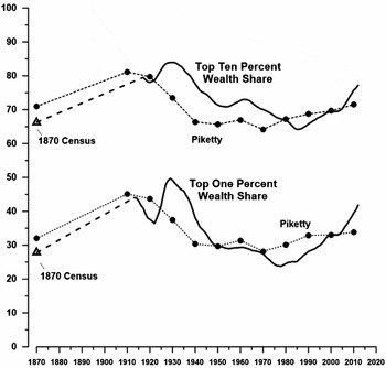
FIGURE 5. Percent of wealth owned by the wealthiest households. Based on Saez-Zucman and the 1870 Census.
TABLE 2. Top wealth shares, household-level unit of observation. Capitalized income tax data, five-year moving average (Saez-Zucman Reference Saez and Zucman2016)

For comparison, the same chart reproduces Piketty's trend. One key difference is that the alternative series starkly reveals a shift to greater equality as the highly progressive income tax took effect during World War I. The highest marginal tax rate reached 77 percent on 1918 incomes more than $1 million (Haig Reference Haig1919: 391). The alternative series also reveals the trend reversal in the 1920s when tax rates on high incomes fell dramatically. The average rate on incomes more than $1 million were lowered from more than 70 percent to 43 percent in 1924 and then again to 24 percent in 1925 (Carter et al. Reference Carter, Gartner, Haines, Olmstead, Sutch and Wright2006: Series Ea772). Piketty entirely misses this swing, a movement that should be important to his claim that “a progressive tax is a crucial component of the social state” and that “it played a central role . . . in the transformation of the structure of inequality in the twentieth century” (Piketty Reference Piketty2014: 497, 505–7, and ch. 14). In fact, the Piketty series gives no indication that there was a marked increase in the concentration of wealth during the 1920s. Because the maldistribution of income and wealth prior to the Great Depression is sometimes mentioned as a fundamental weakness of the economy at the time of the crash, this silence is misleading (Galbraith Reference Galbraith1954: 177–78).
Piketty's straight-line interpolation through the Reagan years misses another swing related to significant changes in the structure of income and estate taxes. This swing was evident in the Kopezuk-Saez estate tax data available to Piketty (see figure 1), so ignoring this movement is surprising. Piketty asserts at the outset of his study that the history of the distribution of wealth “has always been deeply political.” In particular, he suggests, “[T]he resurgence of inequality after 1980 is due largely to the political shifts of the past several decades, especially in regard to taxation and finance” (Piketty Reference Piketty2014: 20). Indeed, there was a significant drop in tax progressivity that started in the late 1970s and intensified during the Reagan administration. The federal government slashed the top marginal income tax rate in a series of steps from 70 percent in 1981 to 28 percent in 1988 (Carter et al. Reference Carter, Gartner, Haines, Olmstead, Sutch and Wright2006: Series Ea826). Estate tax rates were also lowered from a maximum of 70 percent on estates in excess of $5 million in 1981 to 55 percent in 1987 (Luckey Reference Luckey2011: 13–16).
The other remarkable contrast between the alternative series and the trend Piketty presented is that the new series presents a picture of sharply rising inequality over the last 35 years. Twenty-four percent of US wealth was in the hands of the richest 1 percent at the end of the 1970s. By 2012 their share had risen to 42 percent. By contrast the Piketty trend hardly increases from 1990 to 2010. There is an irony here. While intending to demonstrate that inequality has been growing recently, Piketty underestimated the trend.
With the two plots at the top, figure 5 repeats the comparison between the alternative estimates but for the top 10 percent of the wealth distribution.Footnote 21 A key point to note is that the smoothed Saez-Zucman series is a direct measure of the wealth share owned by the top decile. It was not generated by shifting the 1 percent share mechanically upward.
Conclusion
Capital in the Twenty-First Century with its impressive battery of historical statistics and its bold narrative framework has stimulated an outpouring of new and ongoing work, both interpretive and quantitative. That alone is a welcome development. Creating historical time series takes ingenuity, hard work, and an artist's touch. Thomas Piketty and his collaborators have done a great service for social scientists and historians by assembling and organizing dozens of time series relevant to the study of economic inequality. Their statistics stretch back at least two centuries. They include data for the United States and several European countries. They have quantified the distribution of income, the distribution of marketable wealth, and more. (Note, however, this review is concerned only with the distribution of wealth in the United States.)
Economists, perhaps more so than historians, are apt to take historical statistics as given, “all packed up and parceled” ready for interpretation and analysis. They forget that the ingenuity and the artistry that created the spreadsheet of numbers also produces an idiosyncratic picture of the past. Piketty's manipulation and smoothing of the underlying data was designed to dramatize long-run trends without bogging his narrative down with the short-run details of economic history. Piketty referred to these long-period trends in inequality to support a dynamic model of wealth accumulation and inheritance, which he then extrapolated to the future to warn that “the concentration of [wealth] will attain extremely high levels” (Piketty Reference Piketty2014: 26).
This article is limited to examining the underlying data, the methodology, and the judgment Piketty used to produce his estimates of the long-run trends. As far as the American data on wealth is concerned, I found much to question. A quick summary of my findings is provided by the abstract. The objections I raise may not be fatal, but they should require a careful reconsideration of whether the US experience supports Piketty's theories and predictions. For those interested in current trends, it should be noted that evidence, not available to Piketty when he wrote, now indicates that the increase in inequality since the 1970s has been much more dramatic than his diagrams suggest.
Because of his focus on the long run, Piketty's time trends will prove misleading on such issues as the antebellum trend of inequality, the gyrations buffeting the Gilded Age economy, the redistributive impact of President Wilson's progressive income tax, the impact of the Roaring Twenties and the Great Crash on wealth accumulation, and the consequences of the Reagan-era tax cuts. I am sure that Piketty would be the first to agree that social science historians with interests other than his should not employ his numbers uncritically. Researchers interested in such questions should go behind and beneath the graphs in Piketty's book, examine the raw data for themselves, and revise the statistics as necessary to suit their own purpose. That effort, which will hopefully conclude with a better understanding, will take ingenuity, hard work, and artistry.
In a classic essay, the British historian Herbert Butterfield warned “the understanding of the past is not so easy as it is sometimes made to appear” (Reference Butterfield1931: 132). I agree, but that is how science works.
APPENDIX
The 1870 Census of Wealth
The Nature and Reliability of the Data
I have come loaded with statistics . . . Statistics—statistics—why statistics are more precious and useful than any other one thing in this world, except whisky—I mean hymnbooks.
Mark Twain, “Political Speech,” Hartford, October 26, 1880Footnote 22
A census of the population is required by the US Constitution every 10 years to reapportion the House of Representatives. Political tensions were unusually high in anticipation of the census of 1870 and in the aftermath of the Civil War. Before the end of slavery, slaves counted only three-fifths of a person in establishing the size of each congressional district (US Constitution, Article I, Section 2, Clause 3). After emancipation, the freedmen were to be accorded parity with everyone else in the reapportionment. Republican congressmen from the northern states were concerned about the additional seats to be allocated for southern states, which were likely to elect members of the Democratic Party.Footnote 23 While a compromise was sought, the bill authorizing the census was held in abeyance. After the issue was settled by the Fifteenth Amendment in February 1870 giving the former slaves the right to vote as well as to be counted, Congress lost interest in reforms to improve the basic machinery of census taking. Thus, the Census of 1870 was conducted employing the same procedures used in 1860, which in turn had been patterned on those enacted to conduct the Census of 1850 (Anderson Reference Anderson1988: 72–82).
Coverage
Of course, no US census achieves a complete count. Enumerator error and a floating population of vacationers, migrant workers, and homeless conspire to miss many. Young children were more likely to be missed than adults. Live-in servants are probably overlooked with higher frequency than their employers because the respondent for the household may not have understood that nonfamily members should be included as residents of the household. The Census of 1870 has been singled out as especially prone to an undercount particularly in the South because of suspected unsettled conditions in the aftermath of the Civil War and the devastating mortality during and immediately following the conflict (Hacker Reference Hacker2011). Yet a careful analysis based on the IPUMS data files for a sequence of censuses suggest that the undercount in 1870 was not nearly as great as some nineteenth-century observers had claimed. For white males David Hacker suggests that the census included 92.8 percent of the population, only slightly lower than other nineteenth-century censuses. For native-born white males between 25 and 44 the undercount was in the neighborhood of 10 to 12 percent (Hacker Reference Hacker2013: table 1, 88). Roger Ransom and Richard Sutch estimated the undercount of blacks was 6.6 percent (Reference Ransom and Sutch1975: table 1, 8). Of more concern for this study than the lack of complete coverage is the possibility that the undercount biased estimates of the concentration of wealth. Because many of those excluded were young children and the very poorest of adults the likelihood of a serious bias is reduced. If anything, the rich with their substantial dwelling units and their social prominence are likely to have been relatively well counted.
Instructions for the Enumerators
Two questions on wealth were carried over from the 1860 Census. The instructions to the US Assistant Marshalls who enumerated the 1870 Census read:
Property. Column 8 will contain the value of all real estate owned by the person enumerated, without any deduction on account of mortgage or other incumbrance, whether within or without the census subdivision or the county. The value meant is the full market value, known or estimated.
“Personal estate,” column 9, is to be inclusive of all bonds, stocks, mortgages, notes, live stock, plate, jewels, or furniture, but exclusive of wearing apparel. No report will be made when the personal property is under $100.Footnote 24

FIGURE A1.
This reproduces a portion of the enumerator's manuscript for the city of Buffalo, in Erie County, New York.Footnote 25 On lines 8–12 we find the following entries:
Without ignoring the obvious misspellings and abbreviations, this is undoubtedly the household of Samuel L. Clemens (1835–1910), his wife, Olivia, and three servants. Today Mr. Clemens is better known by his pen name, Mark Twain, America's most famous humorist and the author of the novels Adventures of Tom Sawyer (Reference Twain1876) and Adventures of Huckleberry Finn (Reference Twain1885). At the time of the 1870 Census he had just moved to Buffalo to marry Olivia Langdon and to take over the editorship and part ownership of the Buffalo Express. The census recorded his occupation as proprietor of a daily paper. Clemens claimed $10,000 of real estate and his wife recorded $8,000. In his autobiography, dictated many years later, Twain reported that his wife's father “had bought and furnished a new house for us in the fashionable street, Delaware Avenue, and had laid in a cook and housemaids, and a brisk and electric young coachman, an Irishman, Patrick McAleer” (Smith Reference Smith2010: 321; Twain Reference Twain1907).Footnote 26 It is a sample of one, to be sure, but here the written memoire is consistent with the census record.
Reliability
The data on wealth were self-reported. The responses given tend to cluster at round numbers (hundreds or thousands). It is obvious that most are rough estimates. They would have been made by the household member being interviewed and that individual may not have been the best informed. Richard Steckel compared a sample of the 1870 returns from the Massachusetts towns of Boston, Salem, Lexington, Westminster, and Sturbridge with the taxable wealth established that year by the municipality's tax assessor. Judging from the scatter diagram he presents, I conclude the correlation between the two is quite high (Steckel Reference Steckel1994: figure 1, 76).Footnote 27 Steckel reports that the two measures of wealth have similar size distributions with similar Gini coefficients. Based on this comparison, I conclude that the census data will provide an acceptably accurate picture of the top centiles and percentiles of wealth ownership in 1870.
To be clear, there are several cases in which the two values reported by Steckel differed greatly. The majority were when the census reported zero wealth (i.e., total wealth less than $100), but the appraisals for tax purposes were substantial. This discrepancy most likely arises because the enumerator forgot to ask or the informant failed to respond to the question.Footnote 28 There is no evidence, however, to suggest that this problem would lead to a systematic undercounting of wealth at the upper ranks. Today questions about the magnitude of one's wealth might be considered intrusive. But in the mid-nineteenth century sensibilities were more innocent. I consider it likely that respondents made an honest effort to estimate their wealth. As Carroll Wright, one of America's most prominent statisticians of the era, put it:
As soon as a man realizes that he is giving to the world a fact, he feels the necessity of accuracy, and that to distort the information collected would be to commit a crime worse than any ordinary lying, because it would mislead legislators and others and fix a falsehood in the history of the State. (Reference Wright1901: 1–2)
Contemporaries did not think that misreporting of wealth would be a problem. The New York Times (1870) suggested that “the gatherers of census statistics are looked upon as ‘only the census man,’ and many things that would be carefully concealed from the eyes of other visitors are laid bare to him.”
Gross versus Net Wealth
Aside from the exclusion of clothing and the $100 lower-truncation for personal property, the census's definitions of wealth are inclusive and should provide a reasonable estimate of gross wealth. For some purposes, we might prefer net wealth (assets less debts), but for investigating the concentration of wealth and its impact on the public's concerns about equity, merit, and democracy gross wealth is probably the better measure. After all, the poor cottage residents who might be envious or resentful of the mansions of the wealthy are not likely to soften their views when told of the size of the rich man's mortgage.
In any case, in 1870 gross and net worth were more similar than they are today.Footnote 29 In the 1880s and 1890s, less than one-third of homes were mortgaged. The encumbrance was generally between one-third and one-half of the property value (Eichengreen Reference Eichengreen1984; Snowden Reference Snowden1987, Reference Snowden and Carter2006: Reference Snowden, Lamoreaux and Raff399). The 1870 Census was taken before a national mortgage market had developed (Snowden 1995). In that year, mortgages were probably less common, certainly less standardized, and were more often granted by family members, local merchants, and neighbors than by financial intermediaries.
Consanguineal Families
The wealth variable I calculate is the total wealth recorded in the census for all members of the immediate consanguineal family unit living together in the same household. I am presuming that these family members form a single economic unit with shared resources and nonconflicting economic goals and interests.Footnote 30 The immediate consanguineal family is defined to consist of the household head, his spouse, their unmarried children, and resident (and presumably dependent) parents, whether these relationships are by blood, marriage, or adoption. Siblings, other relatives, nonrelatives, domestic servants, and boarders are not included. Thus, the total wealth for the Clemens's household would be the sum of Samuel and Olivia's reports, $32,000.Footnote 31
In 1870 the census did not specifically enquire about the relationship of household members to the head or their marital status. Instead the instructions to the census enumerators specified that within each household, “the names are to be written beginning with the father and mother; or, if either, or both, be dead, begin with some other ostensible head of the family; to be followed, as far as practicable, with the name of the oldest child residing at home, then the next oldest, and so on to the youngest, then the other inmates, lodgers and boarders, laborers, domestics, and servants.” The IPUMS project imputed the relationships using a set of logical rules based on this ordering, the age, sex, and surname of each individual.Footnote 32
Estimating Personal Estate When Blank
To estimate the fraction of total wealth held by the upper echelons in the distribution we need to estimate the total amount of existing wealth in 1870 that was not reported to the census. Not surprisingly, a significant number of households, 36 percent, did not report personal estate. There are two possible reasons for a report of zero personal property. Some will truly have owned less than $100 of movable assets while others simply failed to answer the question. Reports of zero were more common for young and very old households. The higher rates for the young is no doubt because some of these households had yet to begin to save. The higher rates for the old might be because there would be some who had exhausted their stocks of wealth or who transferred what they had to a grown child in exchange for old-age care. Nonreporting was considerably higher, 63 percent, for households where the family head was illiterate.
I have made a rough estimate of the personal estate for any household reporting zero personal estate. To obtain an idea of how much the $100 minimum might exclude, I turned to the reports from the 1860 Census. In that year there was no minimum imposed on the personal estate question. The data recorded in 1860 suggest that a fairly constant average of just less than $50 was reported for ages 24 to 69. Thereafter the average holdings of portable assets fell off sharply, probably reflecting the exhaustion of personal estate in late life. I arbitrarily set the personal estate to $50 for every household that recorded a blank for that question in 1870.Footnote 33 That sum would be equal to several month's pay for a manufacturing worker and seems a reasonable guess for the average amount of cash held between pay days plus the value of modest household possessions and tools of a trade.Footnote 34


