1 INTRODUCTION
The primary goal of any source finding programme is the accuracy of the resulting catalogues. However, sensitive, wide-field telescopes with fast imaging capabilities, mean that additional requirements are being placed on the software that supports these instruments. Thus, source finding programmes need to evolve with the data which they are processing. Source finding programmes are increasingly being required to make effective use of hardware in order to run in near-real time, integrate with a range of software ecosystems, and have the flexibility to support a range of science goals. We group these demands into three categories: correctness, hardware utilisation, and interoperability.
Time domain astronomy places demands on each of these categories and is thus a good exemplar case. Time domain astronomy is an area of great interest to many of the new radio telescopes either in operation [MWA (Tingay et al. Reference Tingay2013), LOFAR (Röttgering Reference Röttgering2003)], in commissioning [ASKAP (Johnston et al. Reference Johnston2008)], under construction [MeerKAT (Jonas Reference Jonas2009)], or in planning (SKAFootnote 1 ). Studies of variable and transient events are almost entirely focused on variations of source flux density with time. For example, the VAST project (Murphy et al. Reference Murphy2013; Banyer, Murphy, & VAST Collaboration Reference Banyer, Murphy, Ballester, Egret and Lorente2012) and the LOFAR Transients key science project (Swinbank et al. Reference Swinbank2015) have both created analysis pipelines to detect variable and transient objects from light curve data. The critical question for such work is then given a sequence of flux densities and associated 1σ error estimates, what is the degree of variability exhibited by each source, and how confident are we that each source is varying or not. The process of creating light curves from catalogue data involves cross-matching sources between different epochs. Accurate cross-matching requires that sources positions and uncertainties are correctly measured and reported. Since false positives in the detection process appear as single epoch transients, the reliability of a source finding programme is of great importance. Determining the degree and confidence of variability depends critically on the uncertainty associated with each flux measurement in a light curve, and thus the accurate reporting of uncertainties is a priority. In short, detecting variable and transient sources requires that the underlying source-finding process can be relied upon. This in turn requires that the image background and noise, the synthesised beam, and the degree to which the data are correlated, are all important in the source-finding and characterisation process. Time domain astronomy is thus limited by the correctness of the catalogues which are extracted from images.
In order to trigger useful follow-up observations of transients, the time between observation and detection needs to be minimised. This means that the speed of a source finding programme can be critical, and so the ability to utilise multiple CPU or GPU cores becomes important.
Finally, a source finding programme will always comprise only a single component in a larger processing pipeline, and so the ease with which the programme can be incorporated into this environment can be the difference between a practical and impractical solution.
Aegean 2.0 aims to address the issues of correctness, hardware utilisation, and interoperability. Hardware utilisation for Aegean has been improved by using multiple processes for the fitting stage. Interoperability has been improved by exposing the core Aegean functionality in a library called AegeanTools, and by allowing for a greater variety of input and output catalogue formats. These two topics are important but their development is not novel and so we do not discuss them in detail. In this paper, we focus on issues of correctness of the output catalogue.
2 WHY 2.0?
Aegean (Hancock et al. Reference Hancock, Murphy, Gaensler, Hopkins and Curran2012b) was developed to tackle some of the shortcomings of the software that was in common use among radio astronomers in c. 2010. Aegean has been upgraded and improved upon since 2012, thanks to input from work such as Huynh et al. (Reference Huynh, Hopkins, Norris, Hancock, Murphy, Jurek and Whiting2012) and Hopkins et al. (Reference Hopkins2015); however, these works focus on simulated images of modest sizes. Running Aegean on data from SKA pathfinders such as MWA/LOFAR/ASKAP, embedded within scientific work-flows, a number of issues have come to light that have needed to be addressed. These issues are related to practical and theoretical requirements inherent in wide-field radio images, and are invisible to the end user of a radio source catalogue. The requirements include the ability to
-
1. correctly fit a model to data which are spatially correlated,
-
2. work on large fields of view where many parameters vary across the image,
-
3. spread processing across multiple cores/nodes in a high performance computing (HPC) environment, and
-
4. integrate into a variety of work-flows.
Whilst some source finding packages address a subset of these issues, prior to Aegean 2.0, no one package was able to address all four at the same time. This paper serves as a point of reference for the many developments of Aegean as well as a more formal description of the new capabilities.
During the production of the GaLactic and Extragalactic All-sky Murchison Widefield Array (GLEAM) survey catalogue (Hurley-Walker et al. Reference Hurley-Walker2017), all four of the above issues came to bear, and thus Aegean was updated accordingly.
In the sections that follow, we focus on the effects of correlated data, estimating bias and uncertainty (Section 4), estimation of background and noise properties (Section 5), incorporating a variable point spread function (PSF) (Section 6), the process of prioritised fitting (Section 7), extended source models (Section 8), and subimage searching (Section 9). We conclude with a summary (Section 10) and future development plans (Section 11).
The three programmes discussed in this paper (Aegean, BANE, and MIMAS) are part of the AegeanTools software suite. AegeanTools is available for download from GitHub,Footnote 2 along with a user guide and application programming interface (API).
3 TEST DATA
Throughout this work, we rely on two test data sets: simulated data and observational data.
A simulated test image was created with the following properties:
-
• The image centre is at (α = 180°, δ = −45°) (the assumed zenith).
-
• The image size is 10k × 10k pixels, comparable to the mosaics generated for the GLEAM survey.
-
• Pixel area is 0.738 arcmin × 0.738 arcmin at the image centre.
-
• Projection is zenithal equal area (ZEA) in order to accurately represent the large area of sky covered.
-
• Pixels below δ = −84° are masked (blank).
-
• The PSF of the image changes with sky coordinates, being circular at the image centre and elongating with increasing zenith angle.
-
• The image noise varies from 0.1 to 0.2 Jy beam−1.
-
• A large scale smooth background varies from −0.5 to 0.5 Jy beam−1.
-
• A population of point sources were injected with a peak flux distribution ranging from 0.1 to 1000 Jy, a source count distribution of N(S)∝S 3/2, and sky density of 14.5 deg−2.
-
• The source population is uniformly distributed in (α, δ).
The simulated image can be downloaded from Zenodo (Hancock Reference Hancock2017), and the code to generate the test image and all figures used in this paper can be found on the AegeanPaper2.0Plots GitHub repository.Footnote 3
The observational data are taken from Hancock et al. (Reference Hancock, Drury, Bell, Murphy and Gaensler2016a, Reference Hancock, Drury, Bell, Murphy and Gaenslerb). We use just the 1997 epoch of observations originally observed as part of the Phoenix project (Hopkins et al. Reference Hopkins, Mobasher, Cram and Rowan-Robinson1998). These data represent real observations, and include calibration errors, uncleaned side-lobes, and a background and noise that changes throughout the image. This data set will allow us to test the performance of Aegean in good but non-ideal conditions. The simulated and observational images are shown in Figure 1.
Figure 1. Test data used in this paper. Upper: The simulated test image. The colour scale has been chosen to exaggerate the large-scale background emission. The injected sources appear as black points. Lower: An image from the Phoenix deep field, epoch of 1997.
4 LEAST-SQUARES FITTING
The aim of least-squares minimisation is to minimise the following target function:
 $$\begin{equation}
T = \left(\mathrm{model}-\mathrm{data}\right)^T\left(\mathrm{model}-\mathrm{data}\right).
\end{equation}$$
$$\begin{equation}
T = \left(\mathrm{model}-\mathrm{data}\right)^T\left(\mathrm{model}-\mathrm{data}\right).
\end{equation}$$
Ordinary least squares is the best linear unbiased estimator for data in which the errors have zero expectation and the data are uncorrelated. Radio images have spatially correlated pixels and thus ordinary least squares is no longer unbiased. The source models that are typically fit (elliptical Gaussians) are non-linear models, and thus iterative methods are required to perform the fit. Even with uncorrelated data, fitting non-linear models results in parameters being biased and correlated.
Knowing the degree to which the data are correlated, we can alter the target function in Equation (1) to be
 $$\begin{equation}
T^\prime = \left(\mathrm{model}-\mathrm{data}\right)^TC^{-1}\left(\mathrm{model}-\mathrm{data}\right),
\end{equation}$$
$$\begin{equation}
T^\prime = \left(\mathrm{model}-\mathrm{data}\right)^TC^{-1}\left(\mathrm{model}-\mathrm{data}\right),
\end{equation}$$
where the matrix C is the covariance matrix. This expression is unbiased for data distributed as a generalised multivariate Gaussian. Equation (1) is correct when C = σ2 I, where I is the identity matrix and σ2 is the variance of the data. This modification of the target function will remove the bias introduced by having correlated data, but will not affect the bias due to non-linear models. We will first discuss how a covariance matrix can be incorporated into current minimisation libraries (4.1), and then discuss ways to estimate the uncertainty and bias in the resulting parameters (4.2.1).
4.1. Including the covariance matrix
One of most commonly used fitting libraries is MINPACK (Moré et al. Reference Moré, Sorensen, Hillstrom, Garbow and Cowell1984). The MINPACK program LMFIT uses the Lavenburg–Marquardt algorithm to perform non-linear least squares fitting, with the target function as per Euation (1). There is no functionality within the MINPACK library to include a modified version of the target function as per Equation (2). The LMFIT function requires a pointer to a user-generated function which must return the vector (model − data), and it is the Euclidean norm of this vector that is then minimised.
The problem that we are faced with is constructing a vector X such that ||X|| = X T X = T′. With this modified vector, it is then possible to use pre-compiled, debugged, optimised, and well-tested code to fit our data.
4.1.1. Calculating the covariance matrix
The covariance of the data in a radio image is due to one of two effects depending on the type of instrument used. A single dish map will have pixels that are correlated due to the primary beam of the instrument, whilst a map made from an interferometer will have pixels that are correlated due to the synthesised beam. In either case, the covariance matrix can be easily calculated using knowledge of the primary and/or synthesised beam. A typical single dish telescope has a primary beam that is well approximated locally by a Gaussian. An interferometer will have a synthesised beam that is some combination of sinc functions, depending on the (u, v) sampling and weighting functions. Ideally, the inverse covariance matrix would match the synthesised or primary beam, projected onto the pixel coordinates in the image. In many cases, the synthesised beam can be approximated locally by an elliptical Gaussian. For a Gaussian beam with shape parameters of (σ x , σ y , θ), we have a covariance matrix which is
 $$\begin{eqnarray}
C_{i,j} &=& \exp \left[\begin{array}{ll}
-\left(\delta x\sin \theta + \delta y\cos \theta \right)^2/2\sigma _x^2\end{array} \right ] \nonumber\\
&& \times \exp \left[\begin{array}{ll} -\left(\delta x\cos \theta - \delta y\sin \theta \right)^2/2\sigma _y^2 \end{array}\right],\nonumber\\
\delta x &= & x_i - x_j, \nonumber\\
\delta y &= & y_i - y_j.
\end{eqnarray}$$
$$\begin{eqnarray}
C_{i,j} &=& \exp \left[\begin{array}{ll}
-\left(\delta x\sin \theta + \delta y\cos \theta \right)^2/2\sigma _x^2\end{array} \right ] \nonumber\\
&& \times \exp \left[\begin{array}{ll} -\left(\delta x\cos \theta - \delta y\sin \theta \right)^2/2\sigma _y^2 \end{array}\right],\nonumber\\
\delta x &= & x_i - x_j, \nonumber\\
\delta y &= & y_i - y_j.
\end{eqnarray}$$
The covariance matrix is thus real valued and symmetric. The inverse of this matrix exists for all values of (σ x , σ y , θ); however for large (σ x , σ y ), the inverse matrix is numerically unstable. In radio astronomy applications, common practice is to use a restoring beam that has a full width half maximum of between 3–5 pixels, corresponding to a σ of between ~1.5–2.2. For these values of σ, the covariance matrix is easily inverted.
In order to incorporate the inverse covariance matrix into the LMFIT routine, we seek a matrix B such that (BX) T BX = X T C −1 X. This is true if B T B = C −1.
4.1.2. Calculating the matrix B
The required matrix B is a root of the matrix C −1, however many such roots exist. For computational reasons, we also require that B is real valued. Since C −1 is real valued, then one of its roots must also be real valued. Using eigen-decomposition, we can construct a matrix Q of the eigen-vectors of C and a diagonal matrix Λ of the eigen-values of C, such that
 $$\begin{equation}
(Q\Lambda )^{-1}Q\Lambda = C.
\end{equation}$$
$$\begin{equation}
(Q\Lambda )^{-1}Q\Lambda = C.
\end{equation}$$
The eigen-values of C are all positive so that we can create a new matrix Σ such that
 $$\begin{equation}
\Sigma _{i,i} = \frac{1}{\sqrt{\Lambda _{i,i}}}.
\end{equation}$$
$$\begin{equation}
\Sigma _{i,i} = \frac{1}{\sqrt{\Lambda _{i,i}}}.
\end{equation}$$
This then gives the identity (QΣ)−1 QΣ = C −1, which means that B = QΣ is a positive square root of the matrix C −1 as required. The matrix B is unitary and real so that B T = B −1. This choice of B then gives
 $$\begin{equation*}
(BX)^TBX = X^TB^TBX = X^T(Q\Sigma )^{-1}Q\Sigma X = X^TC^{-1}X
\end{equation*}$$
$$\begin{equation*}
(BX)^TBX = X^TB^TBX = X^T(Q\Sigma )^{-1}Q\Sigma X = X^TC^{-1}X
\end{equation*}$$
as required.
In practice, the matrix C may have small negative eigen-values, when the synthesised beam is large compared to the pixel size, or when the number of pixels being fit is large. In either case, the matrix Σ is modified to be
 $$\begin{equation}
\Sigma _{i,i} = \frac{1}{\sqrt{|\Lambda _{i,i}|}}.
\end{equation}$$
$$\begin{equation}
\Sigma _{i,i} = \frac{1}{\sqrt{|\Lambda _{i,i}|}}.
\end{equation}$$
4.2. Parameter uncertainty and bias
The minimisation functions provided by MINPACK will return the parameter estimates that minimise the sum of the squares of the vector X, as well as a variance matrix. If we provide the matrix BX as described in the previous sections, then the parameter estimates will not be biased by the correlation in the input data. However, the returned variance (or 1σ error) estimates will not incorporate the effects of the correlated data. Here we discuss the additional uncertainty and bias that is caused by having a non-linear model and correlated data.
4.2.1. Uncertainty
The variance of the resulting fitted parameters is related to the Fisher Information Matrix by σ2 i = (F − 1) i, i . The Fisher Information Matrix for a real-valued generalised Gaussian is given by Van Trees (Reference Van Trees1947):
 $$\begin{equation}
F_{i,j} = \frac{\partial {G}}{\partial x_i}C^{-1}\frac{\partial {G}}{\partial x_j} + \frac{1}{2}\mathrm{tr}\left(C^{-1}\frac{\partial {C}}{\partial x_i}C^{-1}\frac{\partial {C}}{\partial x_j}\right),
\end{equation}$$
$$\begin{equation}
F_{i,j} = \frac{\partial {G}}{\partial x_i}C^{-1}\frac{\partial {G}}{\partial x_j} + \frac{1}{2}\mathrm{tr}\left(C^{-1}\frac{\partial {C}}{\partial x_i}C^{-1}\frac{\partial {C}}{\partial x_j}\right),
\end{equation}$$
where G is the model of interest (an elliptical Gaussian) and C is the covariance matrix. If the covariance of the data is independent of the model parameters x i , as is the case for radio images, the above equation can be reduced to
 $$\begin{equation}
F_{i,j} = \frac{\partial {G}}{\partial x_i}C^{-1}\frac{\partial {G}}{\partial x_j} = \left(J^TC^{-1}J\right)_{i,j},
\end{equation}$$
$$\begin{equation}
F_{i,j} = \frac{\partial {G}}{\partial x_i}C^{-1}\frac{\partial {G}}{\partial x_j} = \left(J^TC^{-1}J\right)_{i,j},
\end{equation}$$
where J is the Jacobian. Thus, the new variance matrix is related to the original variance matrix but with a contribution from the (data) covariance matrix C. Correct estimation of the error on each parameter means that we must replace the variance matrix returned by MINPACK, with the modified matrix (J T C −1 J)−1. Aegean uses the covariance matrix to estimate the uncertainties according to Equation (8).
We use the simulated test data (Section 3) to compare the reported uncertainties with the deviation between the measured and true parameter values. For a population of measurements, the z-score, defined as
 $$\begin{equation}
\frac{\Delta }{\sigma } \equiv \frac{\textrm {measured}-\textrm {true}}{\textrm {uncertainty}},
\end{equation}$$
$$\begin{equation}
\frac{\Delta }{\sigma } \equiv \frac{\textrm {measured}-\textrm {true}}{\textrm {uncertainty}},
\end{equation}$$
will have mean of 0 and variance of 1 if the reported uncertainties are accurately and precisely estimated. With the simulated data, we have access to the true value of each parameter that is being fit for each source and thus it is possible to determine the z-score distribution The z-score distribution can then be used to determine the accuracy to which the uncertainties are being reported.
We explore three methods of calculating errors: using the Fisher information matrix [Equation (8)] with covariance matrix, using the Fisher information matrix without the covariance matrix (i.e. C = I), and the semi-analytic uncertainties derived by Condon (Reference Condon1997). Aegean fits a model to the data in pixel coordinates, which is then transformed into world (sky) coordinates using the world coordinates system (WCS) module from AstroPy (The Astropy Collaboration et al. 2013). In the cases where the Equation (8) is used, the uncertainties are calculated in pixel coordinates, and then transformed into world (sky) coordinates. Condon (Reference Condon1997) describes the uncertainties in both coordinates, and here we use their Equations (21) and (41) to calculate the uncertainties in the world coordinates directly, with a correction for the correlation between data points. Figure 2 shows histograms of Δ/σ for the position, peak flux, and shape parameters for the three methods.
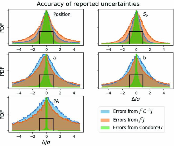
Figure 2. A comparison of the accuracy to which the uncertainties are reported by three different methods. Blue/orange distributions represent uncertainties derived from the FIM using Equation (8) with or without the inverse covariance matrix. The green distribution uses the method described by Condon (Reference Condon1997). The black box indicates a standard deviation of units, which occurs when the uncertainties are accurately reported. Distributions narrower than the black box indicate that the reported uncertainties are too large.
Figure 2 shows that the uncertainties in the shape parameters are not well reported in any of the three methods explored. For the position angle, this can be partially explained by the fact that the position angle has a 2π ambiguity, and is also not defined for circular sources. It is not yet understood why the uncertainties for the semi-major and semi-minor axes are not well described by any of the methods explored. For the position and peak flux, the best method for estimating the uncertainties is to use the covariance matrix, whilst not using the covariance matrix will underestimate the uncertainty, and the description of Condon (Reference Condon1997) will overestimate the uncertainty.
4.2.2. Parameter bias
Refregier et al. (Reference Refregier, Kacprzak, Amara, Bridle and Rowe2012) derive the expected covariance and bias that occurs when using a least-squares algorithm to fit data with a (non-linear) elliptical Gaussian model. They report a parameter variance that is consistent with Equation (8), and additionally report a parameter bias of
 $$\begin{equation}
b[x_i] = -\frac{1}{2}\left(F^{-1}\right)_{ij}\left(F^{-1}\right)_{kl}B_{jkl} + \mathcal {O}\left(\text{SNR}^{-4}\right),
\end{equation}$$
$$\begin{equation}
b[x_i] = -\frac{1}{2}\left(F^{-1}\right)_{ij}\left(F^{-1}\right)_{kl}B_{jkl} + \mathcal {O}\left(\text{SNR}^{-4}\right),
\end{equation}$$
where B ijk is the bias tensor given by
 $$\begin{equation}
B_{ijk} = \sum _p \frac{\partial G}{\partial x_i}\frac{\partial ^2G}{\partial x_j \partial x_k},
\end{equation}$$
$$\begin{equation}
B_{ijk} = \sum _p \frac{\partial G}{\partial x_i}\frac{\partial ^2G}{\partial x_j \partial x_k},
\end{equation}$$
where the subscript p indicates summation over all pixels. Refregier et al. (Reference Refregier, Kacprzak, Amara, Bridle and Rowe2012) show that even in the case of uncorrelated data, to second order in SNR, the best fit position parameters are covariant to a degree determined by the shape parameters, the position and position angle are not biased, the amplitude and major axis are biased high, and the minor axis is biased low.
In an earlier work, Refregier & Brown (Reference Refregier and Brown1998) outline a calculation for the variance and bias of parameters of a non-linear model in the presence of correlated noise. The expected bias is due to two factors: the correlated nature of the data and the non-linear nature of the model being fitted to the data. The inclusion of the inverse covariance matrix into the fitting process should remove the bias due to the correlated nature of the data, however the bias introduced by the non-linearity of the source model will remain.
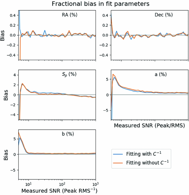
In Figure 3, we measure the bias in five of the model parameters using the simulated data for both fitting methods. The position angle bias is not shown. The bias is calculated as a fraction of the measured value and as a function of the measured SNR for the peak flux, semi-major, and semi-minor axes. For the RA and Dec, the bias is reported as a fraction of the fitted semi-major axis. We make the following observations:
-
• The position of the sources shows no bias in either RA or Dec to within 1% of the semi-major axis.

Figure 3. The bias in fitting each of the six parameters as a function of measured signal-to-noise ratio. The peak flux density (S p) has a small negative bias above about 1 Jy representing an underestimate of the true flux by about 1%. The major axis is biased high as low SNR and then low at higher SNR, whilst the minor axis is always biased high. The RA, Dec, and position angle do not show any consistent biases. The inclusion of the inverse covariance matrix reduces the bias for the major and minor axes at low SNR, but not by a significant amount.
-
• The peak flux and the semi-major and semi-minor axes all show a positive bias of 2–5% at SNR < 10. This bias is not related to the fitting process and is an example of the Eddington bias (Eddington Reference Eddington1913).
-
• The peak flux density has a negative bias that is seen at a SNR of 102, representing a fractional difference of <0.1%.
-
• The semi-minor axis shows no bias aside from the Eddington bias, whilst the semi-major axis shows a residual 1% bias that persists to high SNR.
-
• The 1% bias in the semi-major axis will mean that the source area is also biased high, and that the calculated integrated flux will be biased.
-
• The bias in the integrated flux (not shown) is also high at low SNR but asymptotes to 0 bias at high SNR, indicating that the peak flux and semi-major axis biases cancel out at high SNR.

Figure 3 distinguishes between two fitting methods, with and without the inverse covariance matrix. None of the parameters show significant difference in the bias when using or not using the inverse covariance matrix. As noted previously, the bias due to the non-linearity of our source model cannot be recovered by using the inverse covariance matrix, whilst the bias due to correlated data can be. Thus, we conclude that the cause of bias in the non-linear least squares fitting is dominated by the effects of the non-linear source model. This example demonstrates the asymptotic behaviour of maximum likelihood estimators: The Cramér–Rao bound is met, and the estimator is unbiased, at high SNR but not necessarily at low SNR. At low SNR, the Eddington bias is dominant. The ability to calculate and apply a correction for the bias induced by the spatial covariance of the data has been included in Aegean but is not enabled by default.
5 BACKGROUND AND NOISE ESTIMATION—BANE
Here we compare the background and noise estimation that is performed by Aegean, and that by BANE. We denote the two algorithms as zones (used by Aegean) and grid (used by BANE).
The two algorithms described below share a number of design choices. First, the size of the zone in the zones algorithm and the box in the grid algorithm, are chosen to have width and height that is 30 times the size of the synthesised beam. This choice has been shown by Huynh et al. (Reference Huynh, Hopkins, Norris, Hancock, Murphy, Jurek and Whiting2012) to optimise the completeness and reliability of the extracted compact source catalgoues. Second, the pixel distribution within a region is assumed to contain a contribution from a large-scale background emission, a variance due to noise (a zero mean Gaussian distribution), and real sources (a roughly Poissonian distribution with a very long positive tail). The background and noise properties are typically calculated as the mean and standard deviation of the pixel distribution, however this neglects the contribution from astrophysical sources. Each of these three components are assumed to vary across the image of interest. The goal of the zone and grid algorithms is to estimate the slowly varying background component, the stochastic noise component, without knowledge of, or contamination from, the sources of interest. In the presence of real sources, efforts need to be made to prevent the background and noise parameters from being biased.
5.1. Zones algorithm
The background and noise estimation process that is performed by Aegean is based on a zones algorithm. The zones algorithm divides an image into some number of zones and then computes the background and noise properties of each zone. The pixels within a given zone are used to calculate the 25th, 50th, and 75th percentiles of the flux distribution. The background is taken to be equal to the 50th percentile (the median), whilst the noise is taken to be equal to the inter-quartile range (IQR; 75th–25th percentile) divided by 1.349 (corresponding to 1σ if the pixels follow a Gaussian distribution). Calculating the RMS from the IQR range reduces the bias introduced by source pixels. These background and noise properties are assumed to be constant over a zone, but can vary from zone to zone. This approach is fast to compute, is simple to implement, but will not capture noise and background variations that vary on spatial scales smaller than the size of each zone.
5.2. Grid algorithm
An alternative algorithm is implemented by BANE and it is similar to zones except that it takes a sliding box-car approach. The grid algorithm works on two spatial scales: an inner (grid) scale and an outer (box) scale. The grid algorithm calculates the background and noise properties of all pixels within a box centred on a given grid point. The pixels within a given box are subject to sigma clipping, whereby the mean and standard deviation are calculated, values that are more than 3σ from the calculated mean are masked, and the process is repeated two times. Such sigma-clipping reduces the bias introduced by source pixels, beyond that afforded by the IQR approach. This is similar to the background calculation that is used by SExtractor (Bertin & Arnouts Reference Bertin and Arnouts1996). The next grid point is then selected and the process is repeated. Since the grid points are separated by less than the size of the box, the process naturally provides a somewhat smoothed version of the zones algorithm. Once the background and noise properties have been calculated over a grid of points in the image, a linear interpolation is used to fill in the remainder of the pixel values. If the grid size is set to 1×1 pixels, then this algorithm is equivalent to a box-car filter with sigma clipping. Since radio images are spatially correlated on scales of the synthesised beam, there is little loss of accuracy by increasing the grid size to be 4×4 pixels (a typical synthesised beam size. This small loss of accuracy will then reduce the number of computations required by a factor of 16—greatly increasing the speed of operation. The grid algorithm is slower but more accurate than the zones algorithm, the speed and accuracy can be balanced by adjusting the grid and box sizes. In the case that the background is changing on spatial scales smaller than the box size, the background and noise properties cannot be calculated accurately in a single pass. In such cases, the background must first be calculated, and then the noise can be calculated from the background subtracted data.
The background and noise maps can be stored in a compressed format (not interpolated) and are automatically interpolated at load time by Aegean. This compressed format saves a large amount of storage space at a modest computation cost on load time.
5.3. Algorithm comparison
The zones and grid algorithms are compared in Figure 4 using observational data. The example in question demonstrates that the zones algorithm is, at best, only accurate in the centre of each zone, and that towards the edge of the zone both the background and noise become incorrect. The result of this error is to admit false detections at a rate that is in excess of what could be reasonably expected from simple Gaussian statistics.
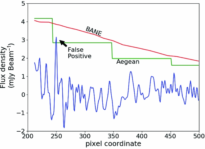
Figure 4. A demonstration of the difference between the Aegean and BANE background and noise maps on the resulting detection threshold. The figure shows a cross-section through an image along one of the pixel axes: flux density as a function of location within the image. The blue line represents the image data. The green and red lines represent the detection threshold (background + 5σ) as calculated using Aegean and BANE characterisations of the background and noise. The difference in the two thresholding techniques results in a false positive when using the Aegean method, but no false positives when using the BANE method.
In Figure 5, we demonstrate the false detections that are due simply to the inadequacies of the zones algorithm, using the observational test real data taken from a single epoch of the Phoenix deep field (Hopkins et al. Reference Hopkins, Mobasher, Cram and Rowan-Robinson1998) studied by Hancock et al. (Reference Hancock, Drury, Bell, Murphy and Gaensler2016b). Figure 5 shows that the false detections occur preferentially towards the edge of the image where the sensitivity is decreasing rapidly due to primary beam effects. In this area, the zones algorithm makes mistakes of the type depicted in Figure 4, and close examination will show that the false detections are indeed at the boundaries of a zone. The background and noise can also be misrepresented in interior image regions near to a bright sources or sources that are not able to be well cleaned. Since this local increase in noise is much smaller than the box over which the noise properties are calculated, there is an increased chance that side-lobes and clean artefacts will rise above the calculated local rms. In a region approximately the size of the calculation box the local rms will be artificially high, meaning that even away from the troublesome source the completeness of the extracted catalogue will be reduced. A typical approach to avoiding the problems of quickly increasing noise is to reduce the area of interest to exclude the outer regions of an image such as shown in Figure 5. Mitigating the effects of the false positives near bright sources in the interior of the image can be achieved with better (u, v) coverage, more careful cleaning, or simply be excising a small area around the problematic sources. These approaches are effective, however they reduce the sky area surveyed. For a given amount of telescope observing time, a reduction in the sky area covered is equivalent to a reduction in sensitivity. Better background and noise estimation is therefore equivalent to an increase in observing sensitivity. For studies interested in detecting transient sources in the image domain, the reduction of false positives translates to a smaller number of false transient candidates, an increased confidence in the transients that are found, and reduced load on the research team.
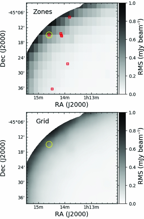
Figure 5. A comparison of two methods for calculating the RMS of an image. Upper: The noise map calculated using the zones algorithm. Lower: The noise map calculated using the grid algorithm. The red X’s represent the location of spurious detections (false positives) due to inaccurate calculation of the background and noise characteristics of the image. The yellow circle denotes the false positive that is depicted in Figure 4.
5.4. Caveats and future work
In the GLEAM survey paper (Hurley-Walker et al. Reference Hurley-Walker2017), it was noted that BANE was not correctly representing the noise properties of the images, and that this was due to the sigma clipping that BANE implements. Whilst this is true, it is not the whole story. The GLEAM survey is sensitivity limited by a combination of side-lobe and classical confusion, resulting in a pixel distribution which is skewed towards positive values. Even after sigma clipping, this skewed distribution means that the standard deviation that BANE calculates is not just the image noise, but a combination of the thermal noise plus a contribution from confusion. The effects of confusion are reproduced in the simulated test image, where the number of sources per synthesised beam increase towards the south celestial pole. In this region of the test image, BANE is not able to accurately reproduce the background and noise properties due to confusion. Currently, BANE makes little use of the WCS header information beyond determining the number of pixels per synthesised beam. The grid/box size that is chosen by BANE is appropriate for the ‘centre’ of the image. For sinusoidal (SIN) projected images, this choice need not change as the beam sampling is typically constant over the entire image, however for large images and other projections this is no longer the case. Indeed the simulated image that was described in Section 3 has a PSF that varies over the image, and so the beam sampling changes accordingly. The result is that the grid/box size is not well chosen for the entire image, and there is a possibility that the spatial filtering will break down, and the separation of background, noise, and signal, can degrade. This is an issue that is currently under development and will be addressed in future versions of BANE.
6 VARIABLE POINT SPREAD FUNCTION
A typical radio image has a PSF which is equal to the synthesised beam, and which is constant across the field of view. At frequencies below ~150 MHz, the ionosphere can induce a lensing effect which can decouple the PSF from the synthesised beam in a manner similar to seeing in optical images (as seen by Loi et al. Reference Loi, Murphy, Cairns, Trott, Hurley-Walker, Feng, Hancock and Kaplan2016). Additionally, stacking or mosaicking of images which are taken under different ionospheric conditions can introduce a blurring effect, due to uncorrected ionospheric shifts (as seen by Hurley-Walker et al. Reference Hurley-Walker2017). A radio interferometer will have a synthesised beam that changes with elevation angle. In a SIN projection with the observing phase centre at the projection centre, the sky to pixel mapping and the synthesised beam will both transform in the same way, at the same rate, and thus the synthesised beam will remain constant in pixel coordinates. For small fields of view, the synthesised beam can be approximated as constant. However, for large fields of view, one or more of the above effects will result in a position-dependent PSF that must be accounted for. Failure to account for a direction-dependent PSF will result in a biased integrated or peak flux measurement, depending on how the flux calibration is calculated. In order to achieve a proper accounting of the peak flux and shape (and thus integrated flux) of a source over the full field of view, source characterisation must be able to use a variable PSF.
In order to allow Aegean to incorporate a variable PSF, we have implemented a PSF model that works in one of two ways. For images that do not suffer from ionospheric blurring, the shape of the synthesised beam can be calculated from the zenith angle, which in turn can be calculated from the latitude of the array. In this case, a user only needs to indicate either the telescope being used or its latitude. Aegean ‘knows’ the latitude of many radio interferometers and so the user can for example use the option – –telescope=MWA. For images that have a position-dependent PSF that is not simply zenith angle dependent, Aegean can be supplied with an auxiliary map that gives the semi-major/semi-minor axes and position angles over the sky. The PSF map is a FITS format image, with three dimensions. The first two dimensions are position (RA/Dec), and the final dimension represents the shape of the PSF in degrees (semi-major, semi-minor, PA). There is no need for the PSF map to be in the same projection or resolution as the input image. Figure 6 shows the PSF map for one week of the GLEAM survey. The AegeanTools package currently does not provide any mechanism by which a PSF map can be produced, however see Hurley-Walker et al. (Reference Hurley-Walker2017) for an example of how this can be done.
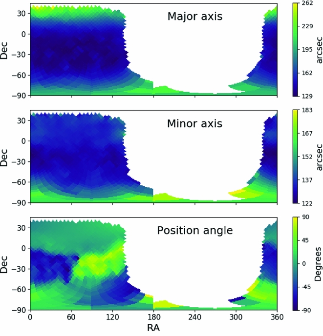
Figure 6. An example PSF map demonstrating the variation of semi-major axis size as a function of position on the sky. The observations contributing to this image are meridian drift scans and thus the semi-minor axis of the synthesised beam should not change with zenith angle. The variations that are seen here are due to differing ionospheric conditions and a blurring effect that is introduced in the mosaicking process. These data drawn from Hurley-Walker et al. (Reference Hurley-Walker2017).
To the best of our knowledge, Aegean is currently the only source finding software that is capable of implementing this feature, despite the fact that it will be critically important for source characterisation with the SKA-Low.
7 PRIORITISED FITTING
Fitting uncertainties are significantly reduced when the number of free parameters are also reduced. If a source is known to exist at a given location, then a user may want to ask ‘What flux is consistent with a source with a given location and shape?’ The traditional approach of recording an upper limit makes statistical analysis difficult, and does not use all of the available data. A new method has been implemented that will allow source characterisation to be achieved independent of the source finding stage. This process is analogous to aperture photometry in optical images, and since it relies on prior information, we use the term prioritised fitting. Prioritised fitting will result in measurements with associated uncertainties, rather than a mix of measurements and limits, making it possible to use a greater variety of statistical methods when analysing the data.
When two or more sources are near to each other, they can become blended. When fitting for the flux of a source that is near to another source, the fitted flux will be biased. In order to avoid this blending bias, sources which are near enough to become blended are grouped and jointly fit. By default, sources which overlap each other at the half power point (have overlapping ellipses) are put into the same group. The model that is fit contains all the sources within a group. Figure 7 shows an example of the regrouping and prioritised fitting.
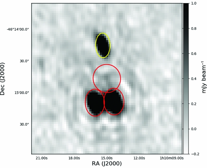
Figure 7. An example of the source regrouping that is performed by Aegean to ensure that overlapping sources are jointly fit. An ellipse represents the location and shape of each component. Three components in the red/lower island are jointly fit in both the blind and prioritised fitting method. The yellow/upper component is fit separately.
The pixels that are included in the fit are selected based on their distance from the source to be fit and the size of said source. The selection of pixels for prioritised fitting is thus different from that which occurs during the normal blind find/characterise operation of aegean. This choice of pixels allows for sources that are below a nominal 5σ detection threshold to be measured. For this reason, it is possible for the prioritised fitting routine to return a negative flux value. Sources that are poorly fit initially, or not well described by an elliptical Gaussian will be poorly measured by a prioritised fit. Due to the possibility that different pixels may be used in the blind and prioritised fitting, the resulting fluxes may differ. However, our tests show that sources that are initially well fit have a prioritised peak flux that is identical to within the reported errors. Figure 8 compares the flux that is measured by Aegean in a blind source finding mode (the default), as compared to that measured with the prioritised fitting mode where only the flux is fit.
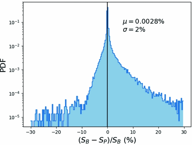
Figure 8. A comparison of the peak flux as measured by Aegean in the blind source finding mode S B or the prioritised fitting mode S P, using the simulated test image. The fluxes agree to within their respective uncertainties, with a variance of just 2%.
Prioritised fits are treated in the same way as the regular (blind) detections. This means that by default the inverse covariance matrix is used in the fitting, the errors are measured according to Section 4.2.1, and the results are reported in the same tabular formats. Aegean generates a universally unique identifier (UUID) for each source in the blind source finding stage, and then copies this UUID during the prioritised fitting. Thus, the light curves or spectral energy distributions can be easily reconstructed by doing an exact match on the UUID key. Matching on UUID instead of position will avoid the many problems and uncertainties associated with cross-matching catalogues.
Since prioritised fitting is a two-step process (find and then remeasure), it is now possible for Aegean to use one image as a detection image, and use a separate image as a measurement image. The following use cases come immediately to mind: variability, spectral studies, and polarisation work. In searching for radio variability, a deep image can be created with all the available data from which a master catalogue can be created. Producing light curves for all the sources present in the deep image is then simply a matter of doing a prioritised fit on each image from each epoch, using the master catalogue as an input. A similar approach can be taken when working with images at multiple frequencies: a single image is chosen as the reference image, and then source fluxes are measured in each of the other images, producing a continuous spectral energy distribution for every source. This is the approach taken for the GLEAM survey (Hurley-Walker et al. Reference Hurley-Walker2017). Finally, even for a single epoch and frequency, prioritised fitting can be used to measure polarised intensity in stokes Q, U, and V images, for sources detected in a stokes I image.
In each of the use cases outlined above, the advantage of prioritised fitting is that every source of interest is assigned a measurement and uncertainty. This means that the resulting light curves, spectral energy distributions, or polarisation states, do not contain limits or censored data. The measurement of source flux may become negative in the low SNR regime, and while this may not be physically meaningful, it is statistically meaningful, and such measurements should be included, for example, when fitting a model spectral energy distribution (Callingham et al. Reference Callingham2017).
Chhetri et al. (Reference Chhetri, Morgan, Ekers, Macquart, Sadler, Giroletti, Callingham and Tingay2017) recently used Aegean to find sources in an image representing the standard deviation of a data cube. These variable sources were then characterised by using prioritised fitting to extract their mean fluxes from an image formed from the mean of the data cube. In this way, the modulation index of the scintillating component was able to be separated from non-scintillating components in sources which may have arcminute scale structure.
8 OTHER SOURCE MODELS
Aegean was designed to find and characterise compact sources. Aegean identifies islands of pixels using a signal to noise threshold. This threshold is applied on the absolute value of the SNR, and thus both positive and negative sources are identified in the source finding phase. By default, only sources with positive SNR are characterised and reported, but Aegean is also able to characterise negative sources. The option – –negative will turn on this feature and allow, for example, both left and right circularly polarised sources to be identified in Stokes V images, in a single pass.
Aegean finds sources based on islands of pixels (Hancock et al. Reference Hancock, Murphy, Gaensler, Hopkins and Curran2012b), fitting one or more components to each of these islands. Diffuse or resolved sources are not well fit by Aegean, however the islands that are identified can be characterised in terms of their position, area, angular extent, and integrated flux. The option – –island will cause Aegean to also report the parameters of pixel islands, both positive and negative. Island properties are written to a separate catalogue, which can be linked to the source catalogue using the island column. For both island and component catalogues, Aegean can write a DS9 region file that identifies exactly which pixels within the image contributed to each island. Figure 9 shows an example of a DS9 visualisation of an island that was characterised by Aegean.
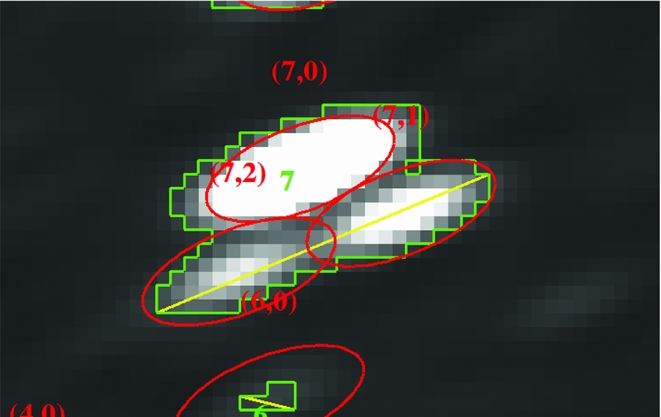
Figure 9. Example of the island characterisation that is available in Aegean. DS9 is used to visualise the extent and location of the island. The red ellipses show the components that were fit with (island, component) labels. The green borders show the pixels that were included in each island with label of the island number. The island number in the islands catalogue can be used to identify which components were fit to this island from the components catalogue. The yellow line indicates the largest angular extent of the island.
9 SUBIMAGE SEARCHING WITH MIMAS
Aegean suffers from a defect that occurs when a large region of an image is included in a single island. The covariance matrix grows as the square of the number of pixels within an island, and the number of sources also increase. Both of these effects cause the fitting of an island to take a very large amount of time, and can cause a crash. There are two solutions to this problem. The first solution is to mask the pixels in an image which would cause a large island to be found. This is typically in regions towards the edge of an image where the noise becomes high, near bright sources that are not able to be cleaned completely, or around extended or resolved sources such as within the Galactic plane. A second solution is to leave the image untouched, but to provide a masking file to Aegean. The masking file will cause Aegean to ignore any islands whose pixels do not fall within the masking region. The second method has the advantage that these regions can be calculated in advance, and a single such mask can be used for many images. By separating the image from the mask, it also means that users no longer need to have masked and unmasked versions of their data on disk. This is the method used by Meyers et al. (Reference Meyers2017) to avoid finding sources near the edge of their survey images. The format of the mask file is a pickle of a python object that is created using the Multi-resolution Image Masking tool for Aegean Software (MIMAS). Figure 10 shows an example of the use of such a mask region to exclude the high noise regions from the observational test image.

Figure 10. Example use of a region mask to constrain the area over which source finding will be performed. The background image is an rms map generated by BANE, with a linear colour scale from 0.1 to 1 mJy beam−1. The black diamonds show the masking region, which are represented by HEALPix pixels of different order. Only islands of sources which overlap the mask region are fit by Aegean.
MIMAS uses a Hierarchical Equal Area isoLatitude Pixelization of a sphere (HEALPix,Footnote 4 Gorski et al. Reference Gorski, Hivon, Banday, Wandelt, Hansen, Reinecke and Bartelman2004), to represent the sky as a set of pixels. Storing sky areas as sets of HEALPix pixels make is possible to combine regions using binary set operations. Currently, MIMAS supports union and difference operations from the command line, but the underlying module (AegeanTools.Regions) is able to support all the set operations provided by the built in set class. Python pickle files are not amenable to easy visualisation, so MIMAS provides two methods for visualisation. First is a Multi-Order Coverage map (MOCFootnote 5 ) as a .FITS file. These MOC files can be easily visualised and manipulated by the Aladin viewer (Bonnarel et al. Reference Bonnarel2000). A second method of visualisation is a region file that is readable by DS9.
10 SUMMARY
We have addressed the issue of fitting non-linear models to correlated data as it applies to radio astronomy images. We have developed a method that accounts for the correlated nature of the data in the fitting process, but found that the resulting fit parameters were not significantly different as a result. The reported parameter uncertainties and calculated biases were presented. We find that including the data covariance matrix in the Fisher information matrix gives the best estimate of the uncertainty in position and peak flux, whilst none of the three methods investigated were able to accurately report uncertainties for the shape parameters. The parameter biases that we detect are dominated by the non-linear nature of the source model and not the data covariance. Aegean has been modified to use the data covariance matrix in the reporting of parameter uncertainties.
We presented an algorithm for estimating the background and noise properties of an image and compared it with more simplistic methods currently in use. We find that the background and noise images created by BANE result in a lower false detection rate, especially in the case where the background or noise properties are changing quickly within an image.
We presented a method of prioritised fitting that allows for a more statistically robust estimate of the flux of a source even when the source is below the classical detection threshold. This prioritised fitting simplifies the analysis of light curves and spectral energy distributions by replacing upper limits with a statistically meaningful measurement and uncertainty. Aegean is able to perform prioritised fitting with a choice of the number of degrees of freedom, and includes a regrouping algorithm that ensures that overlapping sources and components are fit jointly.
Wide-field imaging requires that the local PSF be allowed to vary across the image in a possibly arbitrary manner. We have provided description of how to create a FITS format image that will describe the changing PSF, and Aegean is able to use such an image to correctly characterise sources.
We have developed a method for describing regions of sky of arbitrary complexity, based on the HEALPix projection of the sphere. This method is made available via the MIMAS program, and the region files that it can produce can be used to constrain the area of sky over which Aegean will find sources.
The overall development path for Aegean and BANE has been driven by the current needs of radio astronomers and the anticipated future needs of astronomers working on the SKA.
11 FUTURE DEVELOPMENT PLANS
In order to make better use of the multiple cores available on desktop and HPC machines, Aegean has been modified to spread the process of fitting across multiple cores. BANE was created with a parallel-processing capability from the outset. The multi-processing for both Aegean and BANE is currently made possible via the pprocess moduleFootnote 6 . Spreading the processing across multiple cores is done by forking, and thus the memory usage is multiplied by the number of processes, and there is no capability for spreading across multiple computing nodes within an HPC environment. Work is underway to migrate to an OpenMPIFootnote 7 -based approach which will reduce the total memory usage, and allow the processing to be spread across multiple nodes within an HPC environment. With the many new HPC facilities offering GPU nodes as well as CPU nodes, there is significant motivation for a GPU implementation of both Aegean and BANE and expertise is being sought for such an implementation.
BANE currently works with a square grid that is constant over an image. The ideal grid size is dependent on the image PSF (Huynh et al. Reference Huynh, Hopkins, Norris, Hancock, Murphy, Jurek and Whiting2012) and so we are working on a method by which the grid and box size that is used by BANE will be able to also scale with the image PSF. This development will further improve the performance of Aegean via more accurate background and noise models.
The intended use of Aegean is for continuum images and thus works only on a single image at a time. Source finding and source characterisation are two distinct tasks, and can be performed on separate images. We plan to develop such a capability for Aegean such that source finding can be completed on a detection image, and then characterisation on a separate image, or sequence of images. This will be a hybrid of the current blind finding/characterisation and prioritised fitting that Aegean is able to achieve.
The current ideology that is adopted by Aegean and BANE is that the background, noise, and sources are all independent of each other. This is true of compact continuum images which have been well cleaned. However, image of polarised emission are inherently positive definite, and have a non-Gaussian noise distribution, whereby the noise and signal are not combined linearly, but in quadrature. Thus, the true estimation of the image noise requires knowledge of the sources within the image. This suggests that the background and noise estimation needs to be performed before or in conjunction with the source finding and characterisation process.
A common user request is for Aegean to be able to find sources in image cubes similar to the capability of Duchamp (Whiting & Humphreys Reference Whiting and Humphreys2012). An adjustment to the source model to include a spectral index, and possibly spectral curvature is a first step towards meeting this goal. Image cubes that have a PSF that changes significantly with frequency are now being produced by instruments such as the MWA, which have a large fractional bandwidth. A PSF that changes with frequency can be characterised in a manner similar to that described in Section 6, by adding an additional dimension to the data.
ACKNOWLEDGEMENTS
We acknowledge the work and support of the developers of the following python packages: Astropy (The Astropy Collaboration et al. 2013), Numpy (van der Walt, Colbert, & Varoquaux Reference van der Walt, Colbert and Varoquaux2011), Scipy (Jones et al. Reference Jones2001), and LmFit (Newville et al. Reference Newville2017).
Development of Aegean made extensive use of the following visualisation and analysis packages: DS9,Footnote 8 Topcat (Taylor Reference Taylor, Shopbell, Britton and Ebert2005), and Aladin (Bonnarel et al. Reference Bonnarel2000; Boch & Fernique Reference Boch, Fernique, Manset and Forshay2014).
We thank the following people for their contributions to Aegean whether they be in the form of code, bug reports, or suggested features: Ron Ekers, Jessica Norris, Sharkie, Tara Murphy, Shaoguang Guo, Stefan Duchesne, rmalexan, Josh Marvil, David Kaplan, Yang Lu, Robin Cook, Martin Bell, John Morgan, Christopher Herron, Sarah White, and Rajan Chhetri.
This research made use of Astropy, a community-developed core Python package for Astronomy (The Astropy Collaboration et al. 2013). This research has made use of the VizieR catalogue access tool, CDS, Strasbourg, France. The original description of the VizieR service was published in Ochsenbein, Bauer, & Marcout (Reference Ochsenbein, Bauer and Marcout2000). This research has made use of ‘Aladin sky atlas’ developed at CDS, Strasbourg Observatory, France. Parts of this research were conducted by the Australian Research Council Centre of Excellence for All-sky Astrophysics (CAASTRO), through project number CE110001020. This work was supported by resources provided by The Pawsey Supercomputing Centre with funding from the Australian Government and the Government of Western Australia. This project was undertaken with the assistance of resources and services from the National Computational Infrastructure (NCI), which is supported by the Australian Government.
Additional Software provided by AegeanTools
Aegean, BANE, and MIMAS, are all part of the AegeanTools library. There are additional scripts available as part of this library that are useful and are discussed briefly below.
A AeRes
AeRes is a program that will compute the a residual map when given an input image and a catalogue of sources. AeRes was created to help test and verify the performance of Aegean but has been found to be useful for other purposes, and has thus been made available as part of the AegeanTools package. The intention is that the input catalogue was created by Aegean on the input image. In order to reduce the computational cost of modelling sources, source models are only computed over a small subset of the entire image. The sources can be modelled down to either a given fraction of their peak flux, or to a given SNR (default is SNR = 4), a choice which can be controlled by the user with the – –frac or – –sigma options.
Alternative uses for AeRes include the ability to insert model sources into an image using the – –add option. The simulated test image discussed in Section 3, was constructed in this manner. Alternatively, sources can be masked (pixels set to blank) from an input image using the – –mask option.
Not all of the columns from the Aegean catalogue format are used by AeRes. For users wishing to create their own catalogue outside of Aegean, the following columns are required:
-
• ra (°)
-
• dec (°)
-
• local_rms (Jy)
-
• peak_flux (Jy)
-
• a (arcsec)
-
• b (arcsec)
-
• PA (°)
All other columns may be ignored or set to Null values.
B SR6
As mentioned in Section 5, BANE is able to output compressed versions of the background and noise maps. These maps are significantly smaller than the normal output maps, and differ only in the fact that the final interpolation has not been performed. SR6 (Shrink Ray 6) is a helper tool that was initially created to enable a user to take a background or noise map created by BANE and convert between the compressed and non-compressed versions. The decompression of an already compressed file is done using linear interpolation between pixels on a grid. The compression of a map is implemented as decimation, where by every Nth pixel in a grid is saved. The parameters of the initial image and the compression state are stored in the FITS header with custom keywords of the form BN_XXXX. These same keywords are used when BANE is instructed to write a compressed output. Aegean is able to recognise these keywords upon loading a file and, when present, the interpolation of a background or noise image will be done at load time.