


1 Introduction
A crucial issue in the study of real analytic germs is the choice of a good equivalence relation by which we can distinguish them. One may think about  $C^{r}$-equivalence,
  $r=0,1,\ldots ,\infty ,{\it\omega}$. However, the topological equivalence seems, unlike the complex case, not fine enough: for example, all the germs of the form
  $x^{2m}+y^{2n}$ are topologically equivalent. On the other hand, the
  $C^{1}$-equivalence has already moduli: consider the Whitney family
  $f_{t}(x,y)=xy(y-x)(y-tx)$,
  $t>1$, then
  $f_{t}$ and
  $f_{t^{\prime }}$ are
  $C^{1}$-equivalent if and only if
  $t~=~t^{\prime }$. In [Reference Kuo15], Kuo proposed an equivalence relation for real analytic germs named the blow-analytic equivalence for which, in particular, analytically parametrized family of isolated singularities have a locally finite classification. Roughly speaking, two real analytic germs are said blow-analytically equivalent if they become analytically equivalent after composition with real modifications (e.g., finite successions of blowings-up along smooth centers). With respect to this equivalence relation, Whitney family has only one equivalence class. Slightly stronger versions of blow-analytic equivalence have been proposed so far, by Koike and Parusiński in [Reference Koike and Parusiński13] and Fukui and Paunescu in [Reference Fukui and Paunescu11] for example. An important feature of blow-analytic equivalence is also that we have invariants for this equivalence relation, like the Fukui invariants [Reference Fukui10] and the zeta functions [Reference Koike and Parusiński13] inspired by the motivic zeta functions of Denef and Loeser [Reference Denef and Loeser5] using the Euler characteristic with compact supports as a motivic measure.
The present paper is interested in the study of Nash germs, that is real analytic germs with semialgebraic graph. In [Reference Fichou8], Fichou defined an analog adapted to Nash germs of the blow-analytic equivalence of Kuo in [Reference Kuo15]: two Nash germs are said blow-Nash equivalent if, after composition with Nash modifications, they become analytically equivalent via a Nash isomorphism (if the Nash isomorphism preserves the critical loci of the Nash modifications, it is called a blow-Nash isomorphism). He showed, in particular, that blow-Nash equivalence is an equivalence relation and that it has no moduli for Nash families with isolated singularities. Using as a motivic measure the virtual Poincaré polynomial of McCrory and Parusiński in [Reference McCrory and Parusiński20], extended to the wider category of  ${\mathcal{A}}{\mathcal{S}}$ sets [Reference Kurdyka16] and [Reference Kurdyka and Parusiński17] by Fichou in [Reference Fichou7], one can generalize the zeta functions of Koike and Parusiński in [Reference Koike and Parusiński13]. In [Reference Fichou8], Fichou showed that these latter zeta functions are invariants for blow-Nash equivalence via blow-Nash isomorphisms.
In this paper, we consider Nash germs invariant under right composition with a linear action of a finite group. We define for such germs a generalization of the blow-Nash equivalence of [Reference Fichou8] involving equivariant data. If  $G$ is a finite group acting linearly on
  $\mathbb{R}^{d}$ and trivially on
  $\mathbb{R}$, we say that two equivariant, or invariant, Nash germs
  $f,h:(\mathbb{R}^{d},0)\rightarrow (\mathbb{R},0)$ are
  $G$-blow-Nash equivalent if there exist two equivariant Nash modifications
  ${\it\sigma}_{f}:(M_{f},{\it\sigma}_{f}^{-1}(0))\rightarrow (\mathbb{R}^{d},0)$ and
  ${\it\sigma}_{h}:(M_{h},{\it\sigma}_{h}^{-1}(0))\rightarrow (\mathbb{R}^{d},0)$ of
  $f$ and
  $h$ and an equivariant Nash isomorphism
  ${\rm\Phi}:(M_{f},{\it\sigma}_{f}^{-1}(0))\rightarrow (M_{h},{\it\sigma}_{h}^{-1}(0))$ which induces an equivariant homeomorphism
  ${\it\phi}:(\mathbb{R}^{d},0)\rightarrow (\mathbb{R}^{d},0)$ such that
  $f=h\circ {\it\phi}$ (Definition 2.1). If
  ${\rm\Phi}$ preserves the critical loci of
  ${\it\sigma}_{f}$ and
  ${\it\sigma}_{h}$, we say that
  ${\rm\Phi}$ is an equivariant blow-Nash isomorphism. We consider the equivalence relation generated by the equivariant blow-Nash equivalence, which allows refinement of the nonequivariant blow-Nash classification. For example, consider the germs
  $y^{4}-x^{2}$ and
  $x^{4}-y^{2}$. They are Nash equivalent but we show in Example 4.2 that they are not
  $G$-blow-Nash equivalent via an equivariant blow-Nash isomorphism if
  $G=\{1,s\}$ with
  $s$ the involution given by
  $(x,y)\mapsto (-x,y)$.
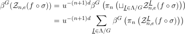
Our main interest is the construction of invariants for  $G$-blow-Nash equivalence via equivariant blow-Nash isomorphism. We associate to any invariant Nash germ its equivariant zeta functions: they are defined using the equivariant virtual Poincaré series of Fichou in [Reference Fichou9] as an equivariant motivic measure on its arc spaces equipped with the induced action of
  $G$ (Section 3.2). It is a generalization of the zeta functions defined in [Reference Fichou7] and [Reference Fichou8], and they are different from the equivariant zeta functions defined in [Reference Fichou9]. We then prove the rationality of the equivariant zeta functions by Denef–Loeser formulas (Propositions 3.12 and 3.17). One has to keep attention on the behavior of the induced actions of
  $G$ on all the spaces involved in the demonstrations of the formulas. A key point is the proof of the validity of Kontsevich “change of variables formula” [Reference Kontsevich14] in this equivariant setting (Proposition 3.14).
Finally, we compute the equivariant zeta functions of several invariant Nash germs (Section 5). We are, in particular, interested in the invariant Nash germs induced from the normal forms of the simple boundary singularities of manifolds with boundary (see [Reference Arnold, Gusein-Zade and Varchenko1]). In a subsequent work, we plan to study the simple boundary singularities of Nash manifolds with boundary and classify them with respect to equivariant blow-Nash equivalence.
We begin this paper by the definition of  $G$-blow-Nash equivalence for
  $G$ a finite group. We also make precise what we mean by an equivariant modification of an invariant Nash germ.
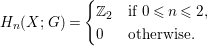
In Section 3, we define the equivariant zeta functions (naive and with signs) of an invariant Nash germ. We first recall the definition of the  $G$-equivariant virtual Betti numbers: they are the unique additive invariants on the category of
  ${\mathcal{A}}{\mathcal{S}}$ sets equipped with an algebraic action of
  $G$ which coincide with the dimensions of equivariant Borel–Moore homology with
  $\mathbb{Z}_{2}$-coefficients (where
  $\mathbb{Z}_{2}$ denotes the field with two elements
  $\mathbb{Z}/2\mathbb{Z}$) on compact nonsingular sets. In Section 3.3, we prove an equivariant version of Kontsevich “change of variables formula” and Denef–Loeser formulas for equivariant zeta functions.
In Section 4, we show that the equivariant zeta functions are invariant under equivariant blow-Nash equivalence via equivariant blow-Nash isomorphisms, illustrating this result with the example of the Nash germs  $y^{4}-x^{2}$ and
  $x^{4}-y^{2}$ invariant under the involution
  $(x,y)\mapsto (-x,y)$. The computation of the equivariant zeta functions of several other invariant Nash germs concludes the paper.
2 Equivariant blow-Nash equivalence
Let  $G$ be a finite group.
We are interested in the study of germs of Nash functions invariant under some linear action of  $G$ on the source space. More precisely, we want to make progress toward the classification of such germs up to equivariant equivalence. We define below in 2.1 some generalization of the blow-Nash equivalence defined by Fichou in [Reference Fichou8], taking into account the equivariant data of this setting.
Let us first make precise definitions in the equivariant setting. Let  $d\geqslant 1$ and equip the affine space
  $\mathbb{R}^{d}$ with a linear action of
  $G$ and the real line
  $\mathbb{R}$ with the trivial action of
  $G$. In this setting, a germ of an equivariant Nash function
  $f:(\mathbb{R}^{d},0)\rightarrow (\mathbb{R},0)$ will be called an equivariant or invariant Nash germ.
An equivariant Nash modification of such a germ  $f$ will be an equivariant proper surjective Nash map
  ${\it\pi}:(M,{\it\pi}^{-1}(0))\rightarrow (\mathbb{R}^{d},0)$ between
  $G$-globally stabilized semialgebraic and analytic neighborhoods of
  ${\it\pi}^{-1}(0)$ in
  $M$ and
  $0$ in
  $\mathbb{R}^{d}$, such that
(1)
 $M$ is a Nash manifold equipped with an algebraic action of $G$ (i.e., an action induced from a regular $G$-action on the Zariski closure of $M$), given by algebraic isomorphisms ${\it\delta}_{g}$, $g\in G$;
(2) the equivariant complexification
${\it\pi}(\mathbb{C}):M(\mathbb{C})\rightarrow \mathbb{C}^{d}$ is an equivariant biholomorphism outside some subset of $M(\mathbb{C})$ of codimension at least $1$, globally stabilized by the complexified action of $G$ on $M(\mathbb{C})$;(3)
${\it\pi}$ is an isomorphism outside the zero locus of $f$;(4) the irreducible components of
$(f\circ {\it\pi})^{-1}(0)$ which are not exceptional divisors of ${\it\pi}$ do not intersect;(5) the action of
$G$ on $M$ preserves globally each exceptional divisor of ${\it\pi}$;(6) the composition
$f\circ {\it\pi}$ and the Jacobian determinant $jac~{\it\pi}$ of ${\it\pi}$ have only normal crossings simultaneously, on which the action of $G$ on $M$ can be locally linearized in the following meaning:Let
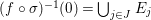
$(f\circ {\it\pi})^{-1}(0)=\bigcup _{j\in J}E_{j}$ be the decomposition of $(f\circ {\it\pi})^{-1}(0)$ into irreducible components. For $I\subset J$, we denote $E_{I}:=\bigcap _{i\in I}E_{i}$. We ask that for any $I\subset J$ with $|I|\leqslant d$, for any element $x$ of $E_{I}$, there exists an affine open neighborhood $U_{x}$ of $x$ in $M$, an affine open neighborhood $V_{x}$ of $0$ in $\mathbb{R}^{d}$, with coordinates $y_{1},\ldots ,y_{d}$ and a Nash isomorphism ${\it\varphi}_{x}:V_{x}\rightarrow U_{x}$ (in the sense of [Reference Fichou7]) such that(a) for all
$i\in I$, there exists $j_{i}\in \{1,\ldots ,d\}$, such that∙
$E_{i}\cap U_{x}={\it\varphi}_{x}(\{y_{j_{i}}=0\}\cap V_{x})$;∙
$f\circ {\it\pi}({\it\varphi}_{x}(y_{1},\ldots ,y_{d}))=unit(y_{1},\ldots ,y_{d})~\prod _{i\in I}y_{j_{i}}^{N_{j_{i}}}$;∙
$jac~{\it\pi}({\it\varphi}_{x}(y_{1},\ldots ,y_{d}))=unit(y_{1},\ldots ,y_{d})~\prod _{i\in I}y_{j_{i}}^{{\it\nu}_{j_{i}}-1}$;
(b) for all
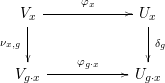
$g\in G$, ${\it\delta}_{g}(E_{i})\cap {\it\delta}_{g}(U_{x})={\it\varphi}_{g\cdot x}(\{y_{j_{i}}=0\}\cap V_{g\cdot x})$;(c) for all
$g\in G$, ${\it\delta}_{g}(U_{x})=U_{g\cdot x}$ and there exists a linear isomorphism ${\it\nu}_{x,g}:\mathbb{R}^{d}\rightarrow \mathbb{R}^{d}$ such that ${\it\nu}_{x,g}(V_{x})=V_{g\cdot x}$ making the following diagram commute:(d) if
${\it\delta}_{g}(E_{I})=E_{I}$, $U_{g\cdot x}=U_{x}$, $V_{g\cdot x}=V_{x}$ and ${\it\varphi}_{g\cdot x}={\it\varphi}_{x}$;(e) for all
$g\in G$, ${\it\nu}_{x,g}$ preserves the intersection of the hyperplanes $\{y_{s}=0\}$, $s\notin \{j_{i},i\in I\}$;(f) for all
$g\in G$, the linear isomorphisms ${\it\nu}_{h\cdot x,g}$, $h\in G$, are all given by the same matrix $A_{x,g}$ in the canonical bases of $\mathbb{R}^{d}\supset V_{h\cdot x}$ and $\mathbb{R}^{d}\supset V_{gh\cdot x}$;(g) all these conditions come from the semialgebraic and analytic isomorphisms between compact semialgebraic and real analytic sets inducing the Nash isomorphisms
${\it\varphi}_{x}$.


Definition 2.1. Let  $f,h:(\mathbb{R}^{d},0)\rightarrow (\mathbb{R},0)$ be two invariant Nash germs. We say that
  $f$ and
  $h$ are
  $G$-blow-Nash equivalent if there exist
∙ two equivariant Nash modifications
${\it\sigma}_{f}:(M_{f},{\it\sigma}_{f}^{-1}(0))\rightarrow (\mathbb{R}^{d},0)$ and ${\it\sigma}_{h}:(M_{h},{\it\sigma}_{h}^{-1}(0))\rightarrow (\mathbb{R}^{d},0)$ of $f$ and $h$, respectively;∙ an equivariant Nash isomorphism
${\rm\Phi}$ between $G$-globally stabilized semialgebraic and analytic neighborhoods $(M_{f},{\it\sigma}_{f}^{-1}(0))$ and $(M_{h},{\it\sigma}_{h}^{-1}(0))$;∙ an equivariant homeomorphism
${\it\phi}:(\mathbb{R}^{d},0)\rightarrow (\mathbb{R}^{d},0)$;


such that the following diagram commutes:
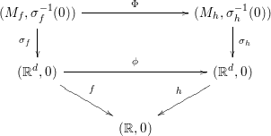
In this case, we say that  ${\it\phi}$ is an equivariant blow-Nash homeomorphism, and if
  ${\rm\Phi}$ preserves the multiplicities of the Jacobian determinant of
  ${\it\sigma}_{f}$ and
  ${\it\sigma}_{g}$ along their exceptional divisors, then we say that
  ${\rm\Phi}$ is an equivariant blow-Nash isomorphism.
∙ If
$G=\{e\}$, the equivariant blow-Nash equivalence is the blow-Nash equivalence defined in [Reference Fichou8].∙ There exist germs being blow-Nash equivalent via a blow-Nash isomorphism without being
$G$-blow-Nash equivalent via an equivariant blow-Nash isomorphism (see Example 4.2).


In the following, we also call  $G$-blow-Nash equivalence (resp.
  $G$-blow-Nash equivalence via an equivariant blow-Nash isomorphism) the equivalence relation generated by the
  $G$-blow-Nash equivalence (resp.
  $G$-blow-Nash equivalence via an equivariant blow-Nash isomorphism) defined in Definition 2.1. Notice that the
  $G$-blow-Nash equivalence can be defined if
  $G$ is an infinite group as well.
3 Equivariant zeta functions
Let  $G$ be a finite group.
We are interested in the classification of Nash germs invariant under right composition with a linear action of  $G$, with respect to the equivariant blow-Nash equivalence. With this in mind, we generalize the zeta functions defined in [Reference Fichou7] to our equivariant setting, using the equivariant virtual Poincaré series defined in [Reference Fichou9]. We show in Proposition 3.12 the rationality of our equivariant zeta functions by a Denef–Loeser formula, which allows us to prove that they are invariants for equivariant blow-Nash equivalence via an equivariant blow-Nash isomorphism (Theorem 4.1).
3.1 Equivariant virtual Poincaré series
In order to define “equivariant” generalizations of the zeta functions for Nash germs, we use an additive invariant defined on all  $G$-
$G$- ${\mathcal{A}}{\mathcal{S}}$ sets, that is Boolean combinations of arc-symmetric sets (see [Reference Kurdyka16] and [Reference Kurdyka and Parusiński17]) equipped with an algebraic action of
  $G$: the equivariant virtual Poincaré series. It is defined in [Reference Fichou9] using the equivariant virtual Betti numbers, which are the unique additive invariant on
  $G$-
$G$- ${\mathcal{A}}{\mathcal{S}}$ sets coinciding with the dimensions of their equivariant homology. In this subsection, we recall the results of Fichou in [Reference Fichou9] about equivariant Betti numbers. We first give the definition of equivariant homology which is a mix of group cohomology and Borel–Moore homology.
Definition 3.1. Let  $\mathbb{Z}_{2}[G]$ denote the group ring of
  $G$ over
  $\mathbb{Z}_{2}$, that is
 $$\begin{eqnarray}\mathbb{Z}_{2}[G]=\left\{\mathop{\sum }_{g\in G}n_{g}g~|~n_{g}\in \mathbb{Z}_{2}\right\}\end{eqnarray}$$
 equipped with the induced ring structure. Consider a projective resolution  $(F_{\ast },{\rm\Delta}_{\ast })$ of
  $\mathbb{Z}_{2}$ by
  $\mathbb{Z}_{2}[G]$-modules, that is vector spaces over
  $\mathbb{Z}_{2}$ equipped with a linear action of
  $G$. Then we define the cohomology
  $H^{\ast }(G,M)$ of the group
  $G$ with coefficients in a
  $\mathbb{Z}_{2}[G]$-module
  $M$ to be the cohomology of the cochain complex
 $$\begin{eqnarray}\left(\text{Hom}_{\mathbb{Z}_{2}[G]}(F_{\ast },M),{\rm\Delta}^{\ast }\right)\end{eqnarray}$$
 where, if  ${\it\varphi}:F_{k}\rightarrow M$ is an equivariant linear morphism,
  ${\rm\Delta}^{k}({\it\varphi}):={\it\varphi}\circ {\rm\Delta}_{k+1}$.
Example 3.2. Let  $G$ be a finite cyclic group of order
  $d$ generated by
  $s$. We denote by
  $N:=\sum _{1\leqslant i\leqslant d}s^{i}$. Then a projective resolution of
  $\mathbb{Z}_{2}$ by
  $\mathbb{Z}_{2}[G]$-modules is given by
 $$\begin{eqnarray}\cdots \rightarrow \mathbb{Z}_{2}[G]\xrightarrow[]{1+s}\mathbb{Z}_{2}[G]\xrightarrow[]{N}\mathbb{Z}_{2}[G]\xrightarrow[]{1+s}\mathbb{Z}_{2}[G]\rightarrow \mathbb{Z}_{2}\rightarrow 0,\end{eqnarray}$$
 where the map  $\mathbb{Z}_{2}[G]\rightarrow \mathbb{Z}_{2}$ associates to an element
  $\sum _{1\leqslant i\leqslant d}n_{i}s^{i}$ of
  $\mathbb{Z}_{2}[G]$ the element
  $\sum _{1\leqslant i\leqslant d}n_{i}$ of
  $\mathbb{Z}_{2}$.
The cohomology of the group  $G$ with coefficients in a
  $\mathbb{Z}_{2}[G]$-module
  $M$ is
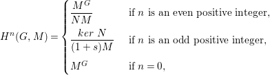 $$\begin{eqnarray}H^{n}(G,M)=\left\{\begin{array}{@{}ll@{}}\displaystyle \frac{M^{G}}{NM}\quad & \text{ if }n\text{ is an even positive integer,}\\ \displaystyle \frac{ker~N}{(1+s)M}\quad & \text{ if }n\text{ is an odd positive integer,}\\ M^{G}\quad & \text{ if }n=0,\end{array}\right.\end{eqnarray}$$
 (where  $M^{G}$ denotes the set of elements of
  $M$ which are fixed by the action of
  $G$). In particular, if
  $G=\mathbb{Z}/2\mathbb{Z}$,
 $$\begin{eqnarray}H^{n}(G,M)=\left\{\begin{array}{@{}ll@{}}{\displaystyle \frac{M^{G}}{(1+s)M}}\quad & \text{ if }n>0,\\ M^{G}\quad & \text{ if }n=0.\end{array}\right.\end{eqnarray}$$
For more details about group cohomology see for instance [Reference Brown3].
The equivariant homology of  $G$-
$G$- ${\mathcal{A}}{\mathcal{S}}$ sets we define below is inspired by [Reference van Hamel21].
Recall that a semialgebraic subset  $S$ of
  $\mathbb{P}^{n}(\mathbb{R})$ is said to be arc-symmetric if every real analytic arc in
  $\mathbb{P}^{n}(\mathbb{R})$ either meets
  $S$ at isolated points or is entirely included in
  $S$. An
  ${\mathcal{A}}{\mathcal{S}}$ set is a Boolean combination of arc-symmetric sets.
Take  $X$ an
  ${\mathcal{A}}{\mathcal{S}}$ set equipped with an algebraic action of
  $G$, that is an action induced from a regular
  $G$-action on its Zariski closure: we call such a set a
  $G$-
$G$- ${\mathcal{A}}{\mathcal{S}}$ set. We can associate to
  $X$ the complex
  $(C_{\ast }(X),\partial _{\ast })$ of its semialgebraic chains with closed supports and
  $\mathbb{Z}_{2}$ coefficients, which computes the Borel–Moore homology of
  $X$ with
  $\mathbb{Z}_{2}$ coefficients, simply denoted by
  $H_{\ast }(X)$ (see Appendix of [Reference McCrory, Parusiński and Friedman19]). The action of
  $G$ on
  $X$ induces by functoriality a
  $G$-action on the chain complex
  $C_{\ast }(X)$ (linear action on chains in each dimension and commutativity with the differential). We then consider the double complex
 $$\begin{eqnarray}(\text{Hom}_{\mathbb{Z}_{2}[G]}(F_{-p},C_{q}(X)))_{p,q\in \mathbb{Z}},\end{eqnarray}$$
 where  $(F_{\ast },{\rm\Delta}_{\ast })$ is a projective resolution of
  $\mathbb{Z}_{2}$ by
  $\mathbb{Z}_{2}[G]$-modules, where the differentials are induced by
  ${\rm\Delta}_{\ast }$ and
  $\partial _{\ast }$.
The equivariant Borel–Moore homology  $H_{\ast }(X;G)$ of
  $X$ (with
  $\mathbb{Z}_{2}$ coefficients) is then by definition the homology of the total complex associated to the above double complex.
Such a double complex induces two spectral sequences that converge to the homology of the associated total complex. In particular, the spectral sequence given by
 $$\begin{eqnarray}E_{p,q}^{2}=H^{-p}(G,H_{q}(X))\Rightarrow H_{p+q}(X;G),\end{eqnarray}$$
 is called the Hochschild–Serre spectral sequence of  $X$ and
  $G$.
$G$.
It gives the following viewpoint on the equivariant Borel–Moore homology: it is a mix of group cohomology and Borel–Moore homology with  $\mathbb{Z}_{2}$ coefficients, involving the geometry of
  $X$, the geometry of the action of
  $G$ and the geometry of the group
  $G$ itself.
Example 3.3. To illustrate how the equivariant geometry is involved in the equivariant homology, let us compute the equivariant homology of the two-dimensional sphere, given by the equation 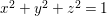 $x^{2}+y^{2}+z^{2}=1$ in
  $\mathbb{R}^{3}$ and denoted by
  $X$, equipped with two different kind of involutions.
Consider first the action given by the central symmetry  $s:(x,y,z)\mapsto (-x,-y,-z)$. If
  $G:=\{1,s\}$, the
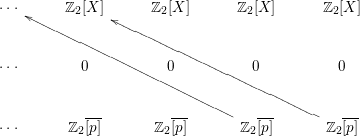
  $E^{2}$-term of the Hochschild–Serre spectral sequence of
  $X$ and
  $G$ is

where  $\overline{[p]}$ is the homology class of the chain
  $[p]$ representing a point
  $p$ of
  $X$: for the sake of simplicity in the computations, we choose
  $p$ to be the point of coordinates
  $(1,0,0)$. We see that the differential
  $d^{2}$ vanishes everywhere and
  $E^{3}$-term is then given by
The image of  $\overline{[p]}$ by the differential
  $d^{3}$ can be obtained by the following procedure. We follow the following “path” in the double complex
  $(\text{Hom}_{\mathbb{Z}_{2}[G]}(F_{-p},C_{q}(X)))_{p,q\in \mathbb{Z}}$:
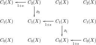
Apply  $1+s$ to the chain
  $[p]$. There exists a semialgebraic chain
  ${\it\gamma}$ of
  $C_{1}(X)$ with boundary
 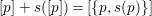 $[p]+s([p])=[\{p,s(p)\}]$: we can choose
  ${\it\gamma}$ to be the chain representing an arc of the equator
  $\{z=0\}$ of
  $X$. The image of
  ${\it\gamma}$ by
  $1+s$ is the chain representing the whole equator
  $\{z=0\}$, which is the semialgebraic boundary of the half-sphere
  $\{z\geqslant 0\}$. Finally, if we apply
  $1+s$ to the chain representing the half-sphere, we obtain the chain
  $[X]$ representing the whole sphere. Therefore,
  $d^{3}(\overline{[p]})=[X]$.
Consequently,
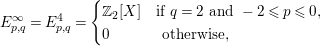 $$\begin{eqnarray}E_{p,q}^{\infty }=E_{p,q}^{4}=\left\{\begin{array}{@{}ll@{}}\mathbb{Z}_{2}[X]\quad & \text{if }q=2\text{ and }-2\leqslant p\leqslant 0,\\ 0\quad & \text{ otherwise,}\end{array}\right.\end{eqnarray}$$
and
 $$\begin{eqnarray}H_{n}(X;G)=\left\{\begin{array}{@{}ll@{}}\mathbb{Z}_{2}\quad & \text{if }0\leqslant n\leqslant 2,\\ 0\quad & \text{otherwise.}\end{array}\right.\end{eqnarray}$$
 Now let  $s$ denote an involution on
  $X$ which is not free: this means there exists at least one point
  $p_{0}$ of
  $X$ that is fixed by
  $s$. If we look at the
  $E^{3}$-term of the Hochschild–Serre spectral sequence of
  $X$ with respect to this action of
  $G=\mathbb{Z}/2\mathbb{Z}$, we see that the differential
  $d^{3}$ vanishes everywhere since
 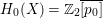 $H_{0}(X)=\mathbb{Z}_{2}\overline{[p_{0}]}$ and
  $(1+s)[p_{0}]=0$. Thus,
  $E^{\infty }=E^{2}$ and
 $$\begin{eqnarray}H_{n}(X;G)=\left\{\begin{array}{@{}ll@{}}\mathbb{Z}_{2}\quad & \text{if }0\leqslant n\leqslant 2,\\ \mathbb{Z}_{2}\oplus \mathbb{Z}_{2}\quad & \text{if }n\leqslant 0,\\ 0\quad & \text{otherwise.}\end{array}\right.\end{eqnarray}$$
∙ When
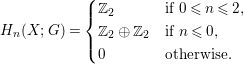
$G=\{e\}$, the equivariant homology of a $G$-${\mathcal{A}}{\mathcal{S}}$ set $X$ is the Borel–Moore homology of $X$.∙ As illustrated in Example 3.3, the equivariant homology groups can be nonzero in negative degree. In the case
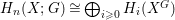
$G=\mathbb{Z}/2\mathbb{Z}$, we actually have $H_{n}(X;G)\cong \bigoplus _{i\geqslant 0}H_{i}(X^{G})$ for $n<0$ (where $X^{G}$ is the set of the points of $X$ which are fixed by the action of $G$).


For more details about equivariant Borel–Moore homology, see [Reference van Hamel21], [Reference Derval6], [Reference Fichou9] and [Reference Priziac18].
The existence and uniqueness of the equivariant Betti numbers are given by the following theorem of Fichou in [Reference Fichou9]. The equivariant virtual Betti numbers and the equivariant virtual Poincaré series are additive invariants under equivariant Nash isomorphisms of  $G$-
$G$- ${\mathcal{A}}{\mathcal{S}}$ sets. By a Nash isomorphism between
  ${\mathcal{A}}{\mathcal{S}}$-sets
  $X_{1}$ and
  $X_{2}$ is meant the restriction of a semialgebraic and analytic isomorphism between compact real analytic and semialgebraic sets
  $Y_{1}$ and
  $Y_{2}$ containing
  $X_{1}$ and
  $Y_{2}$, respectively (see also [Reference Fichou7]).
We use the equivariant virtual Poincaré series as a measure for arc spaces which takes into account equivariant information. In particular, we apply it to the spaces of arcs of an invariant Nash germ and gather these measures in the equivariant zeta functions (Subsection 3.2).
Theorem 3.5. [Reference Fichou9, Theorem 3.9]
Let  $i\in \mathbb{Z}$. There exists a unique map
  ${\it\beta}_{i}^{G}(\cdot )$ defined on
  $G$-
$G$- ${\mathcal{A}}{\mathcal{S}}$ sets and with values in
  $\mathbb{Z}$ such that
(1)
${\it\beta}_{i}^{G}(X_{1})={\it\beta}_{i}^{G}(X_{2})$ if $X_{1}$ and $X_{2}$ are equivariantly Nash isomorphic;(2)
${\it\beta}_{i}^{G}(X)=\dim _{\mathbb{Z}_{2}}H_{i}(X;G)$ if $X$ is a compact nonsingular $G$-${\mathcal{A}}{\mathcal{S}}$ set;(3)
${\it\beta}_{i}^{G}(X)={\it\beta}_{i}^{G}(Y)+{\it\beta}_{i}^{G}(X\setminus Y)$ if $Y\subset X$ is an equivariant closed inclusion;(4)
${\it\beta}_{i}^{G}(V)={\it\beta}_{i}^{G}(\mathbb{R}^{n}\times X)$ with $G$ acting diagonally on the right-hand product, $\mathbb{R}^{n}$ being equipped with the trivial action of $G$, if $V\rightarrow X$ is a $G$-equivariant vector bundle with fiber $\mathbb{R}^{n}$, that is, the restriction to $X$ of a vector bundle with fiber $\mathbb{R}^{n}$ on its Zariski closure $\overline{X}^{Z}$, with a linear $G$-action over the action on $\overline{X}^{Z}$ (this means there exists a finite partition of $\overline{X}^{Z}$ into $G$-globally invariant Zariski constructible sets on which the vector bundle is trivial and the action of $G$ sends linearly a fiber on another).


The map  ${\it\beta}_{i}^{G}(\cdot )$ is unique with these properties and is called the
  $i\text{th}$ equivariant virtual Betti number.
For  $X$ a
$X$ a  $G$-
$G$- ${\mathcal{A}}{\mathcal{S}}$ set, we then denote
 $$\begin{eqnarray}{\it\beta}^{G}(X):=\mathop{\sum }_{i\in \mathbb{Z}}{\it\beta}_{i}^{G}(X)u^{i}\in \mathbb{Z}[u][[u^{-1}]]\end{eqnarray}$$
 the equivariant virtual Poincaré series of  $X$.
$X$.
∙ For
$G=\{e\}$, the equivariant virtual Poincaré series is the virtual Poincaré polynomial defined in [Reference McCrory and Parusiński20].∙ The assumption of finiteness of the group
$G$ is necessary to show the existence of the equivariant virtual Betti numbers. In particular, when $G$ is finite, there always exist an equivariant resolution of singularities ([Reference Villamayor22,Reference Bierstone and Milman2]) and an equivariant compactification (see [Reference Denef and Loeser4]).


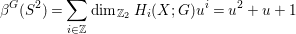
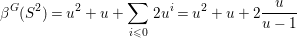
(1) If we consider the sphere
$S^{2}$ equipped with the central symmetry, since $S^{2}$ is compact nonsingular, we have (with$$\begin{eqnarray}{\it\beta}^{G}(S^{2})=\mathop{\sum }_{i\in \mathbb{Z}}\dim _{\mathbb{Z}_{2}}H_{i}(X;G)u^{i}=u^{2}+u+1\end{eqnarray}$$$G=\mathbb{Z}/2\mathbb{Z}$). If now we consider an action of $G$ on $S^{2}$ which fixes at least one point, we have (see Example 3.3).$$\begin{eqnarray}{\it\beta}^{G}(S^{2})=u^{2}+u+\mathop{\sum }_{i\leqslant 0}2u^{i}=u^{2}+u+2\frac{u}{u-1}\end{eqnarray}$$(2) The equivariant virtual Poincaré series of a point is
$\frac{u}{u-1}$ and the equivariant virtual Poincaré series of two points inverted by an action of $G=\mathbb{Z}/2\mathbb{Z}$ is $1$: in both cases, the Hochschild–Serre spectral sequence degenerates at $E^{2}$-term.(3) Let the affine plane
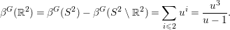
$\mathbb{R}^{2}$ be equipped with an involution $s$. To compute the equivariant virtual Poincaré series ${\it\beta}^{G}(\mathbb{R}^{2})$ (with $G=\{1,s\}$), consider an equivariant one-point compactification of $\mathbb{R}^{2}$. It is equivariantly Nash isomorphic to a sphere $S^{2}$ equipped with an involution fixing at least the point $S^{2}\setminus \mathbb{R}^{2}$. Therefore, $$\begin{eqnarray}{\it\beta}^{G}(\mathbb{R}^{2})={\it\beta}^{G}(S^{2})-{\it\beta}^{G}(S^{2}\setminus \mathbb{R}^{2})=\mathop{\sum }_{i\leqslant 2}u^{i}=\frac{u^{3}}{u-1}.\end{eqnarray}$$(4) Let
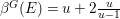
$\mathbb{R}^{2}$ be equipped with an action of $G:=\mathbb{Z}/2\mathbb{Z}$ given by $s:(x,y)\mapsto ({\it\epsilon}x,{\it\epsilon}^{\prime }y)$, with ${\it\epsilon},{\it\epsilon}^{\prime }\in \{-1,1\}$, and $E$ denote the exceptional divisor of the equivariant blowing-up of the plane at $0$. Then, ${\it\beta}^{G}(E)={\it\beta}^{G}(\mathbb{P}^{1})={\it\beta}^{G}(S^{1})$, where the circle $S^{1}$ is equipped with an involution fixing at least one point. Then ${\it\beta}^{G}(E)=u+2\frac{u}{u-1}$ (we compute the Hochschild–Serre spectral sequence of $S^{1}$).


Contrary to the virtual Poincaré polynomial, we do not know the behavior of the equivariant virtual Poincaré series toward products in general case. Nevertheless, we have the following result regarding the equivariant virtual Poincaré series of the product of a  $G$-
$G$- ${\mathcal{A}}{\mathcal{S}}$ set with an affine space. We use the following two properties in the proof of Denef–Loeser formula for the equivariant zeta functions (Subsection 3.3).
Proposition 3.8. (Proposition 3.13 of [Reference Fichou9])
Let  $X$ be any
  $G$-
$G$- ${\mathcal{A}}{\mathcal{S}}$ set and equip the affine variety
  $\mathbb{R}^{n}$ with any algebraic action of
  $G$. If we equip their product with the diagonal action of
  $G$, we have
 $$\begin{eqnarray}{\it\beta}^{G}(\mathbb{R}^{n}\times X)=u^{n}{\it\beta}^{G}(X).\end{eqnarray}$$
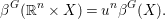
 In particular,  ${\it\beta}^{G}(\mathbb{R}^{n})=\frac{u^{n+1}}{u-1}$.
Lemma 3.9. Let  $X$ be any
  $G$-
$G$- ${\mathcal{A}}{\mathcal{S}}$ set and equip the real line
  $\mathbb{R}$ with any algebraic variety action of
  $G$ stabilizing
  $0$. Now let
  $m\in \mathbb{N}^{\ast }$ and equip the product
  $(\mathbb{R}^{\ast })^{m}\times X$ with the induced diagonal action of
  $G$. Then we have
 $$\begin{eqnarray}{\it\beta}^{G}\left((\mathbb{R}^{\ast })^{m}\times X\right)=(u-1)^{m}{\it\beta}^{G}(X).\end{eqnarray}$$
Proof. We prove this equality by induction on  $m$: we have
 $$\begin{eqnarray}{\it\beta}^{G}\left(\mathbb{R}^{\ast }\times X\right)={\it\beta}^{G}\left(\mathbb{R}\times X\right)-{\it\beta}^{G}\left(\{0\}\times X\right)=(u-1){\it\beta}^{G}(X)\end{eqnarray}$$
 by Proposition 3.8, and, if we assume the property to be true for a fixed  $m\in \mathbb{N}^{\ast }$,
 $$\begin{eqnarray}\displaystyle {\it\beta}^{G}\left((\mathbb{R}^{\ast })^{m+1}\times X\right) & = & \displaystyle {\it\beta}^{G}\left((\mathbb{R}^{\ast })\times (\mathbb{R}^{\ast })^{m}\times X\right)\nonumber\\ \displaystyle & = & \displaystyle (u-1){\it\beta}^{G}\left((\mathbb{R}^{\ast })^{m}\times X\right)=(u-1)^{m+1}{\it\beta}^{G}(X).\nonumber\end{eqnarray}$$
3.2 Equivariant zeta functions
Consider a linear action of  $G$ on
  $\mathbb{R}^{d}$, given by linear isomorphisms
  ${\it\alpha}_{g}$,
  $g\in G$, and equip
  $\mathbb{R}$ with the trivial action of
  $G$. The space
  ${\mathcal{L}}={\mathcal{L}}(\mathbb{R}^{d},0)$ of formal arcs
  $(\mathbb{R},0)\rightarrow (\mathbb{R}^{d},0)$ at the origin of
  $\mathbb{R}^{d}$ is naturally equipped with the induced action of
  $G$ given by
 $$\begin{eqnarray}g\cdot {\it\gamma}:=t\mapsto {\it\alpha}_{g}({\it\gamma}(t))\end{eqnarray}$$
 for all  $g\in G$ and all
  ${\it\gamma}:(\mathbb{R},0)\rightarrow (\mathbb{R}^{d},0)\in {\mathcal{L}}$. Notice that, if
  ${\it\gamma}(t)=a_{1}t+a_{2}t^{2}+\cdots \,$,
  $g\cdot {\it\gamma}(t)={\it\alpha}_{g}(a_{1})t+{\it\alpha}_{g}(a_{2})t^{2}+\cdots \,$ by the linearity of the action.
For all  $n\geqslant 1$, thanks to its linearity, the action of
  $G$ on
  ${\mathcal{L}}$ induces an action on the space
 $$\begin{eqnarray}\displaystyle {\mathcal{L}}_{n} & = & \displaystyle {\mathcal{L}}_{n}(\mathbb{R}^{d},0)\nonumber\\ \displaystyle & = & \displaystyle \left\{{\it\gamma}:(\mathbb{R},0)\rightarrow (\mathbb{R}^{d},0)~|~{\it\gamma}(t)=a_{1}t+a_{2}t^{2}+\cdots +a_{n}t^{n},~a_{i}\in \mathbb{R}^{d}\right\}\nonumber\end{eqnarray}$$
 of arcs truncated at the order  $n+1$. Furthermore, the truncation morphism
  ${\it\pi}_{n}:{\mathcal{L}}\rightarrow {\mathcal{L}}_{n}$ is equivariant with respect to these actions of
  $G$.
$G$.
Consider now an equivariant Nash germ  $f:(\mathbb{R}^{d},0)\rightarrow (\mathbb{R},0)$, that is
  $f$ is invariant under right composition with the linear action of
  $G$. Then, for all
  $n\geqslant 1$, the set
 $$\begin{eqnarray}A_{n}(f):=\left\{{\it\gamma}\in {\mathcal{L}}_{n}~|~f\circ {\it\gamma}(t)=ct^{n}+\cdots \,,~c\neq 0\right\}\end{eqnarray}$$
 of truncated arcs of  ${\mathcal{L}}_{n}$ becoming series of order
  $n$ after left composition with
  $f$ is globally stable under the action of
  $G$ on
  ${\mathcal{L}}_{n}$.
Consequently, we can apply the equivariant virtual Poincaré series to the sets  $A_{n}(f)$, which are Zariski constructible subsets of
  $\mathbb{R}^{nd}$ equipped with an algebraic action of
  $G$, and we define the naive equivariant zeta function
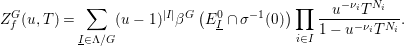
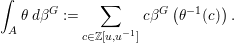
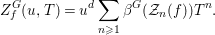
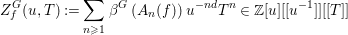 $$\begin{eqnarray}Z_{f}^{G}(u,T):=\mathop{\sum }_{n\geqslant 1}{\it\beta}^{G}\left(A_{n}(f)\right)u^{-nd}T^{n}\in \mathbb{Z}[u][[u^{-1}]][[T]]\end{eqnarray}$$
 of  $f$.
$f$.
Similarly, the sets
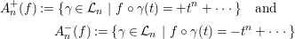 $$\begin{eqnarray}\displaystyle & & \displaystyle A_{n}^{+}(f):=\{{\it\gamma}\in {\mathcal{L}}_{n}~|~f\circ {\it\gamma}(t)=+t^{n}+\cdots \,\}\quad \text{and}\nonumber\\ \displaystyle & & \displaystyle \qquad \qquad A_{n}^{-}(f):=\{{\it\gamma}\in {\mathcal{L}}_{n}~|~f\circ {\it\gamma}(t)=-t^{n}+\cdots \,\}\nonumber\end{eqnarray}$$
 are also stable under the action of  $G$ on
  ${\mathcal{L}}_{n}$ and we define the equivariant zeta functions with signs
  $Z_{f}^{G,+}$ and
  $Z_{f}^{G,-}$ of the invariant Nash germ
  $f$:
$f$:
 $$\begin{eqnarray}Z_{f}^{G,\pm }(u,T):=\mathop{\sum }_{n\geqslant 1}{\it\beta}^{G}\left(A_{n}^{\pm }(f)\right)u^{-nd}T^{n}\in \mathbb{Z}[u][[u^{-1}]][[T]].\end{eqnarray}$$
∙ For
$G=\{e\}$, the equivariant zeta functions are the zeta functions defined in [Reference Fichou7] and [Reference Fichou8].∙ These equivariant zeta functions are different from the equivariant zeta functions defined in [Reference Fichou9].

Example 3.11. (See also [Reference Koike and Parusiński13] and [Reference Fichou7])
Equip the affine line  $\mathbb{R}$ with the linear involution
  $s:x\mapsto -x$. Let
  $k\in \mathbb{N}^{\ast }$ and consider the invariant Nash germ
 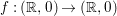 $f:(\mathbb{R},0)\rightarrow (\mathbb{R},0)$ given by
  $f(x)=x^{2k}$.
For all  $n\geqslant 1$, if
  $n$ is not divisible by
  $2k$,
$2k$,  $A_{n}(f)$ is empty, and if
  $n=2km$,
 $$\begin{eqnarray}A_{n}(f)=\left\{{\it\gamma}:(\mathbb{R},0)\rightarrow (\mathbb{R},0)~|~{\it\gamma}(t)=a_{m}t^{m}+\cdots +a_{n}t^{n},~a_{m}\neq 0\right\}\end{eqnarray}$$
 is equivariantly Nash isomorphic to  $\mathbb{R}^{\ast }\times \mathbb{R}^{n-m}$ equipped with the diagonal action of
  $G:=\mathbb{Z}/2\mathbb{Z}$ on each factor induced from the action of
  $s$ on
  $\mathbb{R}$. Therefore, the equivariant virtual Poincaré series of
  $A_{n}(f)$ is
  $(u-1)\frac{u^{n-m+1}}{u-1}=u^{n-m+1}$ if
  $n=2km$ (by Lemma 3.9 and Proposition 3.8),
  $0$ otherwise and we have
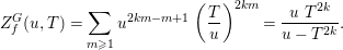 $$\begin{eqnarray}Z_{f}^{G}(u,T)=\mathop{\sum }_{m\geqslant 1}u^{2km-m+1}\left(\frac{T}{u}\right)^{2km}=\frac{u~T^{2k}}{u-T^{2k}}.\end{eqnarray}$$
 Now,  $f$ is positive so
  $Z_{f}^{G,-}=0$, and for
  $n=2km$,
 $$\begin{eqnarray}A_{n}^{+}(f)=\left\{{\it\gamma}:(\mathbb{R},0)\rightarrow (\mathbb{R},0)~|~{\it\gamma}(t)=\pm t^{m}+\cdots +a_{n}t^{n}\right\}\end{eqnarray}$$
 is equivariantly Nash isomorphic to  $\{\pm 1\}\times \mathbb{R}^{n-m}$; hence
  ${\it\beta}^{G}(A_{n}^{+}(f))=u^{n-m}$ (the points
  $-1$ and
  $+1$ are exchanged by the involution
  $s$). Thus,
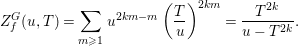 $$\begin{eqnarray}Z_{f}^{G}(u,T)=\mathop{\sum }_{m\geqslant 1}u^{2km-m}\left(\frac{T}{u}\right)^{2km}=\frac{T^{2k}}{u-T^{2k}}.\end{eqnarray}$$
3.3 Denef–Loeser formulas for equivariant zeta functions
In the following proposition 3.12, we show that, as the nonequivariant one in [Reference Fichou7] and [Reference Fichou8], the naive equivariant zeta function is rational. This Denef–Loeser formula for an equivariant modification will allow us to prove that two invariant Nash germs equivariantly blow-Nash equivalent through an equivariant blow-Nash isomorphism have the same naive equivariant zeta function (Theorem 4.1).
We keep the notations from previous Subsection 3.2.
Proposition 3.12. Let  ${\it\sigma}:(M,{\it\sigma}^{-1}(0))\rightarrow (\mathbb{R}^{d},0)$ be an equivariant Nash modification of
  $f$.
$f$.
At first, we keep notations from the nonequivariant case [Reference Fichou8]:
∙ Let
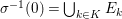
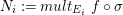
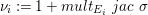
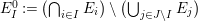
$(f\circ {\it\sigma})^{-1}(0)=\bigcup _{j\in J}E_{j}$ be the decomposition of $(f\circ {\it\sigma})^{-1}(0)$ into irreducible components. Then there exists $K\subset J$ such that ${\it\sigma}^{-1}(0)=\bigcup _{k\in K}E_{k}$.∙ Put
$N_{i}:=mult_{E_{i}}~f\circ {\it\sigma}$ and ${\it\nu}_{i}:=1+mult_{E_{i}}~jac~{\it\sigma}$, and, for $I\subset J$, $E_{I}^{0}:=(\bigcap _{i\in I}E_{i})\setminus (\bigcup _{j\in J\setminus I}E_{j})$.


Now, the action of  $G$ on
  $M$ induces an action of
  $G$ on the set of irreducible components of
  $(f\circ {\it\sigma})^{-1}(0)$. For
  $j_{1},j_{2}\in J$ and
  $g\in G$, we write the equality
  $j_{2}=g\cdot j_{1}$ if
  $E_{j_{2}}=g\cdot E_{j_{1}}$. This induces an action of
  $G$ on the set
  ${\rm\Lambda}$ of nonempty subsets of
  $J$ and we denote by
  $\underline{I}$ the orbit of a nonempty subset
  $I$ of
  $J$.
$J$.
For  $\underline{I}$ in
  ${\rm\Lambda}/G$, we then denote by
  $E_{\underline{I}}^{0}$ the union of the sets
  $E_{g\cdot I}^{0}=g\cdot E_{I}^{0}=\left(\bigcap _{i\in I}g\cdot E_{i}\right)\setminus \left(\bigcup _{j\in J\setminus I}g\cdot E_{j}\right)$,
  $g\in G$ (it is the orbit of
  $E_{I}^{0}$ in
  $M$) and we have the equality
 $$\begin{eqnarray}Z_{f}^{G}(u,T)=\mathop{\sum }_{\underline{I}\in {\rm\Lambda}/G}(u-1)^{|I|}{\it\beta}^{G}\left(E_{\underline{I}}^{0}\cap {\it\sigma}^{-1}(0)\right)\mathop{\prod }_{i\in I}\frac{u^{-{\it\nu}_{i}}T^{N_{i}}}{1-u^{-{\it\nu}_{i}}T^{N_{i}}}.\end{eqnarray}$$
Remark 3.13. For all  $i\in I$ and
  $g\in G$,
  $mult_{g\cdot E_{i}}f\circ {\it\sigma}=mult_{E_{i}}f\circ {\it\sigma}$ and
  $mult_{g\cdot E_{i}}jac~{\it\sigma}=mult_{E_{i}}jac~{\it\sigma}$, thanks to the equivariance of
  $f$ and
  ${\it\sigma}$ (see part (iv) of the proof below).
Proof. The proof is a generalization to the equivariant setting of the proof of Denef–Loeser formula in [Reference Fichou7] and [Reference Fichou8], which uses the theory of motivic integration on arc spaces for arc-symmetric sets (see also [Reference Denef and Loeser5]). The key point is the justification of Kontsevich change of variables formula [Reference Kontsevich14] in our setting.
The proof runs as follows. We define the notion of  $G$-stable subsets of the arc space associated to
  $(\mathbb{R}^{d},0)$ or
  $(M,{\it\sigma}^{-1}(0))$. These sets constitute the measurable sets with respect to a measure defined using the equivariant virtual Poincaré series. Here, we use the good behavior of
  ${\it\beta}^{G}$ with respect to equivariant vector bundles (Proposition 3.8) to justify that this measure is well defined.
This allows one to define an integration with respect to this equivariant measure. We show the validity of the Kontsevich change of variables in the equivariant setting (Proposition 3.14 below) just after the present proof.
This key formula provides us a first intermediate equality for  $Z_{f}^{G}(u,T)$, bringing out some
  ${\mathcal{A}}{\mathcal{S}}$ sets globally invariant under the induced actions of
  $G$, which involve the equivariant Nash modification
  ${\it\sigma}$ of
  $f$.
$f$.
The final step is the computation of the value of the equivariant virtual Poincaré series of these  $G$-
$G$- ${\mathcal{A}}{\mathcal{S}}$ sets in terms of the irreducible components of
  $(f\circ {\it\sigma})^{-1}(0)$.
(i) Equivariant measurability and equivariant integration on arc spaces
We first define a notion of equivariant measurability and equivariant measure in the arc spaces  ${\mathcal{L}}(\mathbb{R}^{d},0)$ and
  ${\mathcal{L}}\left(M,{\it\sigma}^{-1}(0)\right)=\{{\it\gamma}:(\mathbb{R},0)\rightarrow (M,{\it\sigma}^{-1}(0))\text{ formal }\}$. The action of
  $G$ on
  $M$, given by algebraic isomorphisms
  ${\it\delta}_{g}$,
  $g\in G$, induces an action on
  ${\mathcal{L}}(M,{\it\sigma}^{-1}(0))$ by composition. For all
  $n\geqslant 0$, the space
  ${\mathcal{L}}_{n}(M,{\it\sigma}^{-1}(0))$ of arcs truncated at order
  $n+1$ is stable under the action of
  $G$ on
  ${\mathcal{L}}(M,{\it\sigma}^{-1}(0))$ and the
  $(n+1)\text{th}$ order truncating morphism
  ${\it\pi}_{n}:{\mathcal{L}}(M,{\it\sigma}^{-1}(0))\rightarrow {\mathcal{L}}_{n}(M,{\it\sigma}^{-1}(0))$ is equivariant (see part (iv) of the proof).
For convenience, in the following definitions,  ${\mathcal{L}}$ will denote either
  ${\mathcal{L}}(\mathbb{R}^{d},0)$ or
  ${\mathcal{L}}(M,{\it\sigma}^{-1}(0))$.
Now we say that a subset  $A$ of the arc space
  ${\mathcal{L}}$ is
  $G$-stable if there exists
  $n\geqslant 0$ and an
  ${\mathcal{A}}{\mathcal{S}}$-subset
  $C$ of
  ${\mathcal{L}}_{n}$, globally invariant under the algebraic action of
  $G$ on
  ${\mathcal{L}}_{n}$, such that
  $A={\it\pi}_{n}^{-1}(C)$. Notice that a
  $G$-stable set is globally invariant under the action of
  $G$ on
  ${\mathcal{L}}$. Then we define the measure
  ${\it\beta}^{G}(A)$ of a
  $G$-stable set
  $A$ by setting
 $$\begin{eqnarray}{\it\beta}^{G}(A):=u^{-(n+1)d}{\it\beta}^{G}({\it\pi}_{n}(A))\in \mathbb{Z}[u][[u^{-1}]]\end{eqnarray}$$
 for  $n$ big enough.
Let us show that this measure is well-defined. This is actually a consequence of the fact that the truncation projections  $q_{n}:{\mathcal{L}}_{n+1}\rightarrow {\mathcal{L}}_{n}$ are vector bundles with fiber
  $\mathbb{R}^{d}$, the action of
  $G$ sending linearly a fiber on another (for
 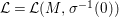 ${\mathcal{L}}={\mathcal{L}}(M,{\it\sigma}^{-1}(0))$, we can cover the compact set
  ${\it\sigma}^{-1}(0)$ by the orbits of a finite number of open affine subsets
  $U_{x}$,
  $x\in {\it\sigma}^{-1}(0)$).
Now, if 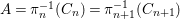 $A={\it\pi}_{n}^{-1}(C_{n})={\it\pi}_{n+1}^{-1}(C_{n+1})$, since
  $q_{n}:C_{n+1}\rightarrow C_{n}$ is a restriction of the
  $G$-equivariant vector bundle
  $q_{n}:{\mathcal{L}}_{n+1}\rightarrow {\mathcal{L}}_{n}$, we have
 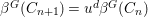 ${\it\beta}^{G}(C_{n+1})=u^{d}{\it\beta}^{G}(C_{n})$ by Theorem 3.5 and Proposition 3.8.
We then define an integral with respect to the measure  ${\it\beta}^{G}$ for maps
  ${\it\theta}$ with source a
  $G$-stable set
  $A$ and
  $\mathbb{Z}[u,u^{-1}]$ as target, with finite image and
  $G$-stable sets as fibers: the integral of
  ${\it\theta}$ over
  $A$ is
 $$\begin{eqnarray}\int _{A}{\it\theta}\,d{\it\beta}^{G}:=\mathop{\sum }_{c\in \mathbb{Z}[u,u^{-1}]}c{\it\beta}^{G}\left({\it\theta}^{-1}(c)\right).\end{eqnarray}$$
(ii) Kontsevich change of variables
Now we state the equivariant version of the change of variables formula in [Reference Kontsevich14] (see also [Reference Denef and Loeser5] and [Reference Fichou7]):
Proposition 3.14. Let  $A$ be
  $G$-stable set of
  ${\mathcal{L}}(\mathbb{R}^{d},0)$ and assume that
  $ord_{t}~jac~{\it\sigma}$ is bounded on
  ${\it\sigma}^{-1}(A)$. Then
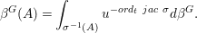 $$\begin{eqnarray}{\it\beta}^{G}(A)=\int _{{\it\sigma}^{-1}(A)}u^{-ord_{t}~jac~{\it\sigma}}d{\it\beta}^{G}.\end{eqnarray}$$
 Here, we denote also by  ${\it\sigma}$ the equivariant map
  ${\mathcal{L}}\left(M,{\it\sigma}^{-1}(0)\right)\rightarrow {\mathcal{L}}(\mathbb{R}^{d},0)~;~{\it\gamma}\mapsto {\it\sigma}\circ {\it\gamma}$. We show Proposition 3.14 after the present proof.
(iii) Applying Kontsevich formula
We use the equivariant version of Kontsevich formula and the additivity of the equivariant virtual Poincaré series to reduce the computation of the naive equivariant zeta function to the computation of the equivariant virtual Poincaré series of  $G$-
$G$- ${\mathcal{A}}{\mathcal{S}}$ sets expressed in terms of the equivariant Nash modification
  ${\it\sigma}$ of
  $f$.
$f$.
First, we give notations to the sets that will appear as the proof goes along, similarly to [Reference Fichou7]. For any  $n\geqslant 1$ and
  $e\geqslant 1$, we put
∙
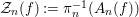
${\mathcal{Z}}_{n}(f):={\it\pi}_{n}^{-1}(A_{n}(f))$;∙
${\mathcal{Z}}_{n}(f\circ {\it\sigma}):={\it\sigma}^{-1}({\mathcal{Z}}_{n}(f))$;∙
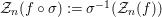
${\rm\Delta}_{e}:=\{{\it\gamma}\in {\mathcal{L}}\left(M,{\it\sigma}^{-1}(0)\right)~|~ord_{t}~jac~{\it\sigma}({\it\gamma}(t))=e\}$;∙
${\mathcal{Z}}_{n,e}(f\circ {\it\sigma}):={\mathcal{Z}}_{n}(f\circ {\it\sigma})\cap {\rm\Delta}_{e}$.


Notice that all the sets  ${\mathcal{Z}}_{n}(f)$,
  ${\mathcal{Z}}_{n}(f\circ {\it\sigma})$,
  ${\rm\Delta}_{e}$ and
  ${\mathcal{Z}}_{n,e}(f\circ {\it\sigma})$ are globally invariant under the actions of
  $G$ on arc spaces, notably because
  ${\it\sigma}$ is an equivariant Nash modification (see also step (iv) below).
First, since all the sets  ${\mathcal{Z}}_{n}(f)$ are by definition
  $G$-stable, we can consider their equivariant measure
  ${\it\beta}^{G}({\mathcal{Z}}_{n}(f))=u^{-(n+1)d}{\it\beta}^{G}(A_{n}(f))$ and write
 $$\begin{eqnarray}Z_{f}^{G}(u,T)=u^{d}\mathop{\sum }_{n\geqslant 1}{\it\beta}^{G}({\mathcal{Z}}_{n}(f))T^{n}.\end{eqnarray}$$
 We then apply the equivariant Kontsevich change of variables formula to compute  ${\it\beta}^{G}({\mathcal{Z}}_{n}(f))$ for all
  $n\geqslant 1$. Indeed, there exists
  $c\in \mathbb{N}$ such that for all
  $n\geqslant 1$,
  ${\mathcal{Z}}_{n}(f\circ {\it\sigma})$ is the finite disjoint union
  $\cup _{e\leqslant cn}{\mathcal{Z}}_{n,e}(f\circ {\it\sigma})$ (see [Reference Fichou7]): in particular, for all
  $n\geqslant 1$,
  $ord_{t}~jac~{\it\sigma}$ is bounded on
 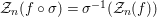 ${\mathcal{Z}}_{n}(f\circ {\it\sigma})={\it\sigma}^{-1}({\mathcal{Z}}_{n}(f))$ and we can apply Proposition 3.14 to obtain
 $$\begin{eqnarray}{\it\beta}^{G}({\mathcal{Z}}_{n}(f))=\int _{{\it\sigma}^{-1}({\mathcal{Z}}_{n}(f))}u^{-ord_{t}~jac~{\it\sigma}}d{\it\beta}^{G}=\mathop{\sum }_{e\leqslant cn}u^{-e}{\it\beta}^{G}\left({\mathcal{Z}}_{n,e}(f\circ {\it\sigma})\right).\end{eqnarray}$$
 Moreover, if  $n\geqslant 1$ and
  $e\leqslant cn$, for any arc
  ${\it\gamma}$ in
  ${\mathcal{Z}}_{n,e}(f\circ {\it\sigma})$ (more generally in
  ${\mathcal{L}}(M,{\it\sigma}^{-1}(0))$), there exists
  $I\subset J$ such that
 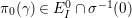 ${\it\pi}_{0}({\it\gamma})\in E_{I}^{0}\cap {\it\sigma}^{-1}(0)$, and more particularly, there exists
  $\underline{I}\in {\rm\Lambda}/G$ such that
 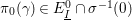 ${\it\pi}_{0}({\it\gamma})\in E_{\underline{I}}^{0}\cap {\it\sigma}^{-1}(0)$.
Consequently, we can write the  $G$-stable set
  ${\mathcal{Z}}_{n,e}(f\circ {\it\sigma})$ as the disjoint union of the sets
  ${\mathcal{Z}}_{n,e}^{\underline{I}}(f\circ {\it\sigma}):={\mathcal{Z}}_{n,e}(f\circ {\it\sigma})\cap {\it\pi}_{0}^{-1}(E_{\underline{I}}^{0}\cap {\it\sigma}^{-1}(0))$,
  $\underline{I}\in {\rm\Lambda}/G$, and we have
 $$\begin{eqnarray}\displaystyle {\it\beta}^{G}({\mathcal{Z}}_{n,e}(f\circ {\it\sigma})) & = & \displaystyle u^{-(n+1)d}{\it\beta}^{G}\left({\it\pi}_{n}\left(\sqcup _{\underline{I}\in {\rm\Lambda}/G}{\mathcal{Z}}_{n,e}^{\underline{I}}(f\circ {\it\sigma})\right)\right)\nonumber\\ \displaystyle & = & \displaystyle u^{-(n+1)d}\mathop{\sum }_{\underline{I}\in {\rm\Lambda}/G}{\it\beta}^{G}\left({\it\pi}_{n}\left({\mathcal{Z}}_{n,e}^{\underline{I}}(f\circ {\it\sigma})\right)\right)\nonumber\end{eqnarray}$$
(in the last equality, we used the additivity of the equivariant virtual Poincaré series).
Finally, we have
 $$\begin{eqnarray}Z_{f}^{G}(u,T)=\mathop{\sum }_{n\geqslant 1}u^{-nd}T^{n}\mathop{\sum }_{e\leqslant cn}u^{-e}\mathop{\sum }_{\underline{I}\in {\rm\Lambda}/G}{\it\beta}^{G}\left({\it\pi}_{n}\left({\mathcal{Z}}_{n,e}^{\underline{I}}(f\circ {\it\sigma})\right)\right),\end{eqnarray}$$
 where 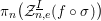 ${\it\pi}_{n}({\mathcal{Z}}_{n,e}^{\underline{I}}(f\circ {\it\sigma}))$ is the
  $G$-
$G$- ${\mathcal{A}}{\mathcal{S}}$ set
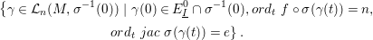 $$\begin{eqnarray}\displaystyle & & \displaystyle \left\{{\it\gamma}\in {\mathcal{L}}_{n}(M,{\it\sigma}^{-1}(0))~|~{\it\gamma}(0)\in E_{\underline{I}}^{0}\cap {\it\sigma}^{-1}(0),ord_{t}~f\circ {\it\sigma}({\it\gamma}(t))=n,\right.\nonumber\\ \displaystyle & & \displaystyle \qquad \qquad \qquad \qquad \left.ord_{t}~jac~{\it\sigma}({\it\gamma}(t))=e\right\}.\nonumber\end{eqnarray}$$
 (iv) Computation of 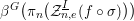 ${\it\beta}^{G}({\it\pi}_{n}({\mathcal{Z}}_{n,e}^{\underline{I}}(f\circ {\it\sigma})))$
Let  $n\geqslant 1$,
  $e\leqslant nc$ and
  $\underline{I}\in {\rm\Lambda}/G$ (such that
  $E_{I}\neq \emptyset$). First, we cover the compact set
  $E_{I}$ by a finite union of open affine subsets
  $U_{x_{r}}$,
  $x_{r}\in E_{I}$,
  $r=1,\ldots ,m$. We can then write
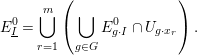 $$\begin{eqnarray}E_{\underline{I}}^{0}=\mathop{\bigcup }_{r=1}^{m}\left(\mathop{\bigcup }_{g\in G}E_{g\cdot I}^{0}\cap U_{g\cdot x_{r}}\right).\end{eqnarray}$$
We are going to compute the equivariant virtual Poincaré series of
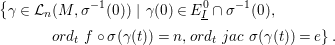 $$\begin{eqnarray}\displaystyle & & \displaystyle \left\{{\it\gamma}\in {\mathcal{L}}_{n}(M,{\it\sigma}^{-1}(0))~|~{\it\gamma}(0)\in E_{\underline{I}}^{0}\cap {\it\sigma}^{-1}(0),\right.\nonumber\\ \displaystyle & & \displaystyle \qquad \quad \left.~ord_{t}~f\circ {\it\sigma}({\it\gamma}(t))=n,ord_{t}~jac~{\it\sigma}({\it\gamma}(t))=e\right\}.\nonumber\end{eqnarray}$$
 Consider an arc  ${\it\gamma}$ in this last set and assume, without any loss of generality, that
 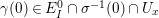 ${\it\gamma}(0)\in E_{I}^{0}\cap {\it\sigma}^{-1}(0)\cap U_{x}$ with
  $x\in \{x_{1},\ldots ,x_{m}\}$. For all
  $i\in I$, we have
∙
$E_{i}\cap U_{x}={\it\varphi}_{x}(\{y_{j_{i}}=0\}\cap V_{x})$;∙
$f\circ {\it\sigma}({\it\varphi}_{x}(y_{1},\ldots ,y_{d}))=unit(y_{1},\ldots ,y_{d})~\prod _{i\in I}y_{j_{i}}^{N_{i}}$;∙
$jac~{\it\sigma}({\it\varphi}_{x}(y_{1},\ldots ,y_{d}))=unit(y_{1},\ldots ,y_{d})~\prod _{i\in I}y_{j_{i}}^{{\it\nu}_{i}-1}$.


We can assume  $U_{x}$ and
  $V_{x}$ are Nash isomorphic
  ${\mathcal{A}}{\mathcal{S}}$-sets such that the above unit Nash functions are nowhere zero on
  $V_{x}$ (by intersecting
  $V_{x}$ with the orbit under
  $G$ of the respective complements of their zero sets which are
  ${\mathcal{A}}{\mathcal{S}}$-sets).
Let  $g\in G$. For
  $i\in I$, the action of
  $g$ on
  $M$ sends an irreducible component
  $E_{i}$ locally described in
  $V_{x}$ by the equation
  $y_{j_{i}}=0$ on the irreducible component
  $E_{g\cdot i}$ locally described in
  $V_{g\cdot x}$ by the same equation
  $y_{j_{i}}=0$. Therefore, after same relevant permutations of coordinates in the source and target spaces, the matrix of
  ${\it\nu}_{x,g}:\mathbb{R}^{d}\supset V_{x}\rightarrow \mathbb{R}^{d}\supset V_{g\cdot x}$ becomes of the form
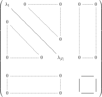
where all the  ${\it\lambda}_{j}$’s are nonzero (recall the definition of an equivariant Nash modification of
  $f$ in Section 2).
In particular, for all  $i\in I$,
∙
$N_{g\cdot i}=N_{i}$;∙
${\it\nu}_{g\cdot i}={\it\nu}_{i}$;∙ if
${\it\gamma}(t)={\it\varphi}_{x}(({\it\gamma}_{1}(t),\ldots ,{\it\gamma}_{d}(t)))$ and if we denote $k_{i}({\it\gamma}):=ord_{t}~{\it\gamma}_{j_{i}}(t)$ for all $i\in I$, $k_{i}(g\cdot {\it\gamma}(t))=k_{i}({\it\gamma})$;


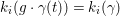
so that there is an equivariant Nash isomorphism between
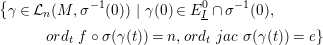 $$\begin{eqnarray}\displaystyle & & \displaystyle \left\{{\it\gamma}\in {\mathcal{L}}_{n}(M,{\it\sigma}^{-1}(0))~|~{\it\gamma}(0)\in E_{\underline{I}}^{0}\cap {\it\sigma}^{-1}(0),\right.\nonumber\\ \displaystyle & & \displaystyle \qquad \quad \left.ord_{t}~f\circ {\it\sigma}({\it\gamma}(t))=n,ord_{t}~jac~{\it\sigma}({\it\gamma}(t))=e\right\}\nonumber\end{eqnarray}$$
and
 $$\begin{eqnarray}\mathop{\sqcup }_{k\in A(n,e)}\left\{{\it\gamma}\in {\mathcal{L}}_{n}(M,{\it\sigma}^{-1}(0))~|~{\it\gamma}(0)\in E_{\underline{I}}^{0}\cap {\it\sigma}^{-1}(0),ord_{t}~{\it\gamma}_{j_{i}}(t)=k_{i},~i\in I\right\},\end{eqnarray}$$
 with  $A(n,e):=\{k\in \mathbb{N}^{d}~|~\sum _{i\in I}k_{i}N_{i}=n,~\sum _{i\in I}k_{i}({\it\nu}_{i}-1)=e\}$. Consequently, the equivariant virtual Poincaré series of these sets are equal.
Let  $k\in A(n,e)$. We compute now the equivariant virtual Poincaré series of the set
 $$\begin{eqnarray}W_{k}:=\left\{{\it\gamma}\in {\mathcal{L}}_{n}(M,{\it\sigma}^{-1}(0))~|~{\it\gamma}(0)\in E_{\underline{I}}^{0}\cap {\it\sigma}^{-1}(0),ord_{t}~{\it\gamma}_{j_{i}}(t)=k_{i},i\in I\right\}.\end{eqnarray}$$
We write it as the difference of
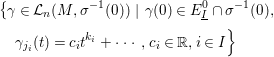 $$\begin{eqnarray}\displaystyle & & \displaystyle \left\{{\it\gamma}\in {\mathcal{L}}_{n}(M,{\it\sigma}^{-1}(0))~|~{\it\gamma}(0)\in E_{\underline{I}}^{0}\cap {\it\sigma}^{-1}(0),\right.\nonumber\\ \displaystyle & & \displaystyle \quad \left.{\it\gamma}_{j_{i}}(t)=c_{i}t^{k_{i}}+\cdots \,,c_{i}\in \mathbb{R},i\in I\right\}\nonumber\end{eqnarray}$$
 and the union over  $l\in I$ of the sets
 $$\begin{eqnarray}\left\{{\it\gamma}\in {\mathcal{L}}_{n}(M,{\it\sigma}^{-1}(0))~|~{\it\gamma}(0)\in E_{\underline{I}}^{0}\cap {\it\sigma}^{-1}(0),{\it\gamma}_{j_{l}}(t)=0\times t^{k_{l}}+\cdots \,\right\}.\end{eqnarray}$$
Thanks to the additivity of the equivariant virtual Poincaré series, we are then reduced to compute the equivariant virtual Poincaré series of
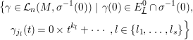 $$\begin{eqnarray}\displaystyle & & \displaystyle \left\{{\it\gamma}\in {\mathcal{L}}_{n}(M,{\it\sigma}^{-1}(0))~|~{\it\gamma}(0)\in E_{\underline{I}}^{0}\cap {\it\sigma}^{-1}(0),\right.\nonumber\\ \displaystyle & & \displaystyle \left.\quad {\it\gamma}_{j_{l}}(t)=0\times t^{k_{l}}+\cdots \,,l\in \{l_{1},\ldots ,l_{s}\}\right\}\nonumber\end{eqnarray}$$
 for any  $\{l_{1},\ldots ,l_{s}\}\subset I$. Considering the restriction to such a set of the projection
  ${\it\pi}_{0}$ onto
  $E_{\underline{I}}^{0}\cap {\it\sigma}^{-1}(0)$, we see that this is a
  $G$-equivariant vector bundle over
  $E_{\underline{I}}^{0}\cap {\it\sigma}^{-1}(0)$ with fibers isomorphic to
  $\mathbb{R}^{|I|-s}\left(\prod _{i\in I}\mathbb{R}^{n-k_{i}}\right)\left(\mathbb{R}^{n}\right)^{d-|I|}$.
Therefore,
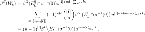 $$\begin{eqnarray}\displaystyle {\it\beta}^{G}(W_{k}) & = & \displaystyle {\it\beta}^{G}(E_{\underline{I}}^{0}\cap {\it\sigma}^{-1}(0))u^{|I|+nd-\mathop{\sum }_{i\in I}k_{i}}\nonumber\\ \displaystyle & & \displaystyle -\,\mathop{\sum }_{s\in \{1,\ldots ,|I|\}}(-1)^{s+1}\binom{|I|}{s}{\it\beta}^{G}\left(E_{\underline{I}}^{0}\cap {\it\sigma}^{-1}(0)\right)u^{|I|-s+nd-\mathop{\sum }_{i\in I}k_{i}}\nonumber\\ \displaystyle & = & \displaystyle (u-1)^{|I|}{\it\beta}^{G}(E_{\underline{I}}^{0}\cap {\it\sigma}^{-1}(0))u^{nd-\mathop{\sum }_{i\in I}k_{i}}.\nonumber\end{eqnarray}$$
As a consequence,
 $$\begin{eqnarray}{\it\beta}^{G}({\it\pi}_{n}\left({\mathcal{Z}}_{n,e}^{\underline{I}}(f\circ {\it\sigma})\right))=\mathop{\sum }_{k\in A(n,e)}(u-1)^{|I|}{\it\beta}^{G}\left(E_{\underline{I}}^{0}\cap {\it\sigma}^{-1}(0)\right)u^{nd-\mathop{\sum }_{i\in I}k_{i}}.\end{eqnarray}$$
(v) Conclusion of the proof
Substituting (2) in the equality (1) of step (iii), we get
 $$\begin{eqnarray}Z_{f}^{G}(u,T)=\mathop{\sum }_{\underline{I}\in {\rm\Lambda}/G}(u-1)^{|I|}{\it\beta}^{G}\left(E_{\underline{I}}^{0}\cap {\it\sigma}^{-1}(0)\right)\mathop{\sum }_{n\geqslant 1}\mathop{\sum }_{e\leqslant cn}\mathop{\sum }_{k\in A(n,e)}u^{-e-\mathop{\sum }_{i\in I}k_{i}}T^{n}.\end{eqnarray}$$
 As in [Reference Fichou7], we write the sum  $\sum _{n\geqslant 1}\sum _{e\leqslant cn}\sum _{k\in A(n,e)}u^{-e-\sum _{i\in I}k_{i}}T^{n}$ as the product
 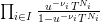 $\prod _{i\in I}\frac{u^{-{\it\nu}_{i}}T^{N_{i}}}{1-u^{-{\it\nu}_{i}}T^{N_{i}}}$ and we obtain the Denef–Loeser formula
 $$\begin{eqnarray}Z_{f}^{G}(u,T)=\mathop{\sum }_{\underline{I}\in {\rm\Lambda}/G}(u-1)^{|I|}{\it\beta}^{G}\left(E_{\underline{I}}^{0}\cap {\it\sigma}^{-1}(0)\right)\mathop{\prod }_{i\in I}\frac{u^{-{\it\nu}_{i}}T^{N_{i}}}{1-u^{-{\it\nu}_{i}}T^{N_{i}}}.\end{eqnarray}$$
We next prove the equivariant version of Kontsevich change of variables (Proposition 3.14), which is a key tool in the demonstration of the above Denef–Loeser formula. In order to achieve this goal, we need the following lemma which is an equivariant Nash analog to [Reference Denef and Loeser5, Lemma 3.4] (see also [Reference Fichou8, Lemma 2.11]):
Lemma 3.15. Let  $h:(M,h^{-1}(0))\rightarrow (\mathbb{R}^{d},0)$ be an equivariant proper surjective Nash map such that the action of
  $G$ on
  $M$ is locally linear around
  $h^{-1}(0)$, that is, corresponds locally to a linear
  $G$-action, in
  $G$-globally invariant affine open charts of
  $M$.
$M$.
For all  $e\geqslant 1$, set
 $$\begin{eqnarray}{\rm\Delta}_{e}:=\left\{{\it\gamma}\in {\mathcal{L}}(M,h^{-1}(0))~|~ord_{t}~jac~h({\it\gamma}(t))=e\right\}\end{eqnarray}$$
 and for all  $n\geqslant 1$,
 $$\begin{eqnarray}{\rm\Delta}_{e,n}:={\it\pi}_{n}({\rm\Delta}_{e}),\end{eqnarray}$$
 and denote by  $h_{n}$ the equivariant map
  ${\it\pi}_{n}\circ h:{\mathcal{L}}_{n}(M,h^{-1}(0))\rightarrow {\mathcal{L}}_{n}(\mathbb{R}^{d},0)$.
If  $n\geqslant 2e$, then
  $h_{n}({\rm\Delta}_{e,n})$ is an
  ${\mathcal{A}}{\mathcal{S}}$ set, globally invariant under the action of
  $G$ on
  ${\mathcal{L}}_{n}(\mathbb{R}^{d},0)$, and
  $h_{n}$ is an equivariantly piecewise trivial fibration over
  $h_{n}({\rm\Delta}_{e,n})$, with
  $G$-globally invariant
  ${\mathcal{A}}{\mathcal{S}}$ sets as pieces, with fiber
  $\mathbb{R}^{e}$ (more precisely
  $h_{n}^{-1}(h_{n}({\rm\Delta}_{e,n}))\rightarrow h_{n}({\rm\Delta}_{e,n})$ is a
  $G$-equivariant vector bundle with fiber
  $\mathbb{R}^{e}$).
Remark 3.16. The details of this fibration are given at the end of the proof below.
Proof of Lemma 3.15.
Fix  $e\geqslant 1$ and
  $n\geqslant 2e$.
The fact that  $h_{n}({\rm\Delta}_{e,n})$ is an
  ${\mathcal{A}}{\mathcal{S}}$ set is given by the nonequivariant result of Fichou in [Reference Fichou8, Lemma 2.11]. Since
  ${\rm\Delta}_{e,n}$ is globally invariant under the action of
  $G$ on
  ${\mathcal{L}}_{n}(M,h^{-1}(0))$, so is the set
  $h_{n}({\rm\Delta}_{e,n})$ under the action of
  $G$ on
  ${\mathcal{L}}_{n}(\mathbb{R}^{d},0)$ because
  $h_{n}$ is equivariant.
In the proof of the second assertion of the lemma, we refer to the proof of [Reference Denef and Loeser5, Lemma 3.4], replacing the terms “regular maps” by “Nash maps” and “constructible sets” by “ ${\mathcal{A}}{\mathcal{S}}$ sets” (see also [Reference Fichou8]).
Consider an equivariant section  $s:{\mathcal{L}}_{n}(\mathbb{R}^{d},0)\rightarrow {\mathcal{L}}(\mathbb{R}^{d},0)$ of
  ${\it\pi}_{n}$. We have
  $s(h_{n}({\rm\Delta}_{e,n}))\subset h({\rm\Delta}_{e})$ and
  $h^{-1}$ is well defined on
  $h({\rm\Delta}_{e})$ (because
  $h({\it\gamma}_{1})\neq h({\it\gamma}_{2})$ if
  ${\it\gamma}_{1}\neq {\it\gamma}_{2}$ with
  ${\it\gamma}_{1}\in {\rm\Delta}_{e}$), Nash and equivariant, so one can construct the equivariant mapping
 $$\begin{eqnarray}{\it\theta}:h_{n}({\rm\Delta}_{e,n})\rightarrow {\rm\Delta}_{e}~;~{\it\gamma}\mapsto h^{-1}(s({\it\gamma})).\end{eqnarray}$$
 It is an equivariantly piecewise morphism: this means there exists a finite partition of the domain of  ${\it\theta}$ into
  ${\mathcal{A}}{\mathcal{S}}$ sets globally invariant under the action of
  $G$ on
  ${\mathcal{L}}_{n}(\mathbb{R}^{d},0)$, such that the restriction of
  ${\it\theta}$ to each piece is an equivariant Nash map, that is induced by an equivariant semialgebraic and analytic map.
One can then use the map  ${\it\theta}$ to express the fiber of an arc
  ${\it\gamma}$ of
  $h_{n}({\rm\Delta}_{e,n})$ under
  $h_{n}$:
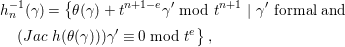 $$\begin{eqnarray}\displaystyle & & \displaystyle h_{n}^{-1}({\it\gamma})=\left\{{\it\theta}({\it\gamma})+t^{n+1-e}{\it\gamma}^{\prime }\text{mod }t^{n+1}~|~{\it\gamma}^{\prime }\text{formal and }\right.\nonumber\\ \displaystyle & & \displaystyle \left.\quad (Jac~h({\it\theta}({\it\gamma}))){\it\gamma}^{\prime }\equiv 0\text{ mod }t^{e}\right\},\nonumber\end{eqnarray}$$
 which can be identified to a linear subspace of  $\mathbb{R}^{de}$ of dimension
  $e$. Furthermore, the action of
  $g\in G$ sending the fiber
  $h_{n}^{-1}({\it\gamma})$ on the fiber
  $h_{n}^{-1}(g\cdot {\it\gamma})$ is given by the matrix
  $A_{x,g}$ for some
  $x\in h^{-1}(0)$.
Therefore, there exists a finite partition of  $h_{n}({\rm\Delta}_{e,n})$ into globally
  $G$-invariant
  ${\mathcal{A}}{\mathcal{S}}$ subsets
  $(S_{i})_{i=1,\ldots ,m}$ of
  ${\mathcal{L}}_{n}(\mathbb{R}^{d},0)$, such that for any
  $i\in \{1,\ldots ,m\}$,
  $h_{n}^{-1}(S_{i})$ is a
  $G$-
$G$- ${\mathcal{A}}{\mathcal{S}}$ subset of
  ${\mathcal{L}}_{n}(M,h^{-1}(0))$, Nash isomorphic to
  $S_{i}\times \mathbb{R}^{e}$, the action of
  $G$ sending linearly a fiber on another.◻
Proof of Proposition 3.14.
We are now ready to prove the equivariant Kontsevich change of variables formula. We are going to compute the integral against the measure  ${\it\beta}^{G}$ of the map
 $$\begin{eqnarray}{\it\zeta}:{\it\sigma}^{-1}(A)\rightarrow \mathbb{Z}[u,u^{-1}]~;~{\it\gamma}\mapsto u^{-ord_{t}~jac~{\it\sigma}({\it\gamma})}\end{eqnarray}$$
 over  ${\it\sigma}^{-1}(A)$, and show that it equals
  ${\it\beta}^{G}(A)$.
We have
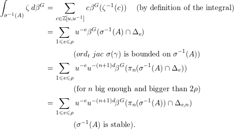 $$\begin{eqnarray}\displaystyle \int _{{\it\sigma}^{-1}(A)}{\it\zeta}\,d{\it\beta}^{G} & = & \displaystyle \mathop{\sum }_{c\in \mathbb{Z}[u,u^{-1}]}c{\it\beta}^{G}({\it\zeta}^{-1}(c))\text{ (by definition of the integral)}\nonumber\\ \displaystyle & = & \displaystyle \mathop{\sum }_{1\leqslant e\leqslant {\it\rho}}u^{-e}{\it\beta}^{G}({\it\sigma}^{-1}(A)\cap {\rm\Delta}_{e})\nonumber\\ \displaystyle & & \displaystyle \quad ~~~~(ord_{t}~jac~{\it\sigma}({\it\gamma})\text{ is bounded on }{\it\sigma}^{-1}(A))\nonumber\\ \displaystyle & = & \displaystyle \mathop{\sum }_{1\leqslant e\leqslant {\it\rho}}u^{-e}u^{-(n+1)d}{\it\beta}^{G}({\it\pi}_{n}({\it\sigma}^{-1}(A)\cap {\rm\Delta}_{e}))\nonumber\\ \displaystyle & & \displaystyle \quad ~~~~(\text{for }n\text{ big enough and bigger than }2{\it\rho})\nonumber\\ \displaystyle & = & \displaystyle \mathop{\sum }_{1\leqslant e\leqslant {\it\rho}}u^{-e}u^{-(n+1)d}{\it\beta}^{G}({\it\pi}_{n}({\it\sigma}^{-1}(A))\cap {\rm\Delta}_{e,n})\nonumber\\ \displaystyle & & \displaystyle \quad ~~~~({\it\sigma}^{-1}(A)\text{ is stable}).\nonumber\end{eqnarray}$$
 Now fix  $1\leqslant e\leqslant {\it\rho}$. We have the equality of sets
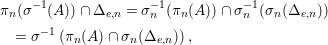 $$\begin{eqnarray}\displaystyle & & \displaystyle {\it\pi}_{n}({\it\sigma}^{-1}(A))\cap {\rm\Delta}_{e,n}={\it\sigma}_{n}^{-1}({\it\pi}_{n}(A))\cap {\it\sigma}_{n}^{-1}({\it\sigma}_{n}({\rm\Delta}_{e,n}))\nonumber\\ \displaystyle & & \displaystyle \quad ={\it\sigma}^{-1}\left({\it\pi}_{n}(A)\cap {\it\sigma}_{n}({\rm\Delta}_{e,n})\right),\nonumber\end{eqnarray}$$
 where  ${\it\sigma}_{n}={\it\pi}_{n}\circ {\it\sigma}$. The equality
 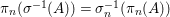 ${\it\pi}_{n}({\it\sigma}^{-1}(A))={\it\sigma}_{n}^{-1}({\it\pi}_{n}(A))$ comes from the stability of
  $A$ and the fact that
  ${\it\pi}_{n}\circ {\it\sigma}\circ {\it\pi}_{n}={\it\pi}_{n}\circ {\it\sigma}$ on
  ${\mathcal{L}}(M,h^{-1}(0))$, and we use [Reference Fichou8, Lemma 2.12] to show that
 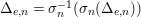 ${\rm\Delta}_{e,n}={\it\sigma}_{n}^{-1}({\it\sigma}_{n}({\rm\Delta}_{e,n}))$ (recall that
  $n\geqslant 2e$).
We then compute  ${\it\beta}^{G}\left({\it\sigma}_{n}^{-1}\left({\it\pi}_{n}(A)\cap {\it\sigma}_{n}\left({\rm\Delta}_{e,n}\right)\right)\right)$ using the fact that, by previous Lemma 3.15,
  ${\it\sigma}_{n}$ is an equivariantly piecewise trivial fibration over
  ${\it\sigma}_{n}({\rm\Delta}_{e,n})$ and more precisely that
  ${\it\sigma}_{n}^{-1}\left({\it\pi}_{n}(A)\cap {\it\sigma}_{n}\left({\rm\Delta}_{e,n}\right)\right)\rightarrow {\it\pi}_{n}(A)\cap {\it\sigma}_{n}\left({\rm\Delta}_{e,n}\right)$ is a restriction of the
  $G$-equivariant vector bundle
  ${\it\sigma}_{n}^{-1}\left({\it\sigma}_{n}\left({\rm\Delta}_{e,n}\right)\right)\rightarrow {\it\sigma}_{n}\left({\rm\Delta}_{e,n}\right)$ with fiber
  $\mathbb{R}^{e}$, so that
 $$\begin{eqnarray}{\it\beta}^{G}\left({\it\sigma}_{n}^{-1}\left({\it\pi}_{n}(A)\cap {\it\sigma}_{n}\left({\rm\Delta}_{e,n}\right)\right)\right)=u^{e}{\it\beta}^{G}\left({\it\pi}_{n}(A)\cap {\it\sigma}_{n}({\rm\Delta}_{e,n})\right).\end{eqnarray}$$
Consequently,
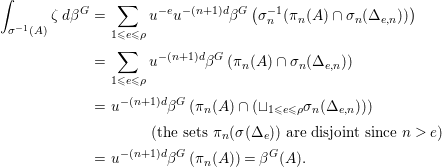 $$\begin{eqnarray}\displaystyle \int _{{\it\sigma}^{-1}(A)}{\it\zeta}\,d{\it\beta}^{G} & = & \displaystyle \mathop{\sum }_{1\leqslant e\leqslant {\it\rho}}u^{-e}u^{-(n+1)d}{\it\beta}^{G}\left({\it\sigma}_{n}^{-1}({\it\pi}_{n}(A)\cap {\it\sigma}_{n}({\rm\Delta}_{e,n}))\right)\nonumber\\ \displaystyle & = & \displaystyle \mathop{\sum }_{1\leqslant e\leqslant {\it\rho}}u^{-(n+1)d}{\it\beta}^{G}\left({\it\pi}_{n}(A)\cap {\it\sigma}_{n}({\rm\Delta}_{e,n})\right)\nonumber\\ \displaystyle & = & \displaystyle u^{-(n+1)d}{\it\beta}^{G}\left({\it\pi}_{n}(A)\cap (\sqcup _{1\leqslant e\leqslant {\it\rho}}{\it\sigma}_{n}({\rm\Delta}_{e,n}))\right)\nonumber\\ \displaystyle & & \displaystyle \qquad ~~(\text{the sets }{\it\pi}_{n}({\it\sigma}({\rm\Delta}_{e}))\text{ are disjoint since }n>e)\nonumber\\ \displaystyle & = & \displaystyle u^{-(n+1)d}{\it\beta}^{G}\left({\it\pi}_{n}(A)\right)={\it\beta}^{G}(A).\nonumber\end{eqnarray}$$
 Notice that we used the surjectivity of the map  ${\it\sigma}_{n}:{\mathcal{L}}_{n}(M,{\it\sigma}^{-1}(0))\rightarrow {\mathcal{L}}_{n}(\mathbb{R}^{d},0)$, which comes from the arc lifting property of a real modification (see, e.g., [Reference Fukui and Paunescu11]).◻
Next, we state the Denef–Loeser formula for the equivariant zeta functions with signs. As in the nonequivariant case (see [Reference Fichou7] and [Reference Fichou8]), we have to consider coverings of the spaces  $E_{I}^{0}$. However, in our equivariant setting, it is necessary to consider coverings of the orbits of these spaces under the induced action of
  $G$.
$G$.
Proposition 3.17. Keep the notations and assumptions of Proposition 3.12. We can write the equivariant zeta functions with signs of  $f$ as a rational fraction in terms of its equivariant Nash modification
  ${\it\sigma}$. Precisely, we have the formula
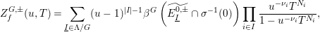 $$\begin{eqnarray}Z_{f}^{G,\pm }(u,T)=\mathop{\sum }_{\underline{I}\in {\rm\Lambda}/G}(u-1)^{|I|-1}{\it\beta}^{G}\left(\widetilde{E_{\underline{I}}^{0,\pm }}\cap {\it\sigma}^{-1}(0)\right)\mathop{\prod }_{i\in I}\frac{u^{-{\it\nu}_{i}}T^{N_{i}}}{1-u^{-{\it\nu}_{i}}T^{N_{i}}},\end{eqnarray}$$
 where, for  $\underline{I}\in {\rm\Lambda}/G$,
  $\widetilde{E_{\underline{I}}^{0,+}}$ and
  $\widetilde{E_{\underline{I}}^{0,-}}$ are
  $G$-coverings of
  $E_{\underline{I}}^{0}$.
Remark 3.18. We define the spaces  $\widetilde{E_{\underline{I}}^{0,\pm }}$ in the proof below, making precise how the action of
  $G$ on
  $M$ induces an action on them.
Proof. To prove the Denef–Loeser formula for equivariant zeta functions with signs, we follow the same first steps as in the proof of Proposition 3.12, and we are led to write
 $$\begin{eqnarray}Z_{f}^{G,\pm }(u,T)=\mathop{\sum }_{n\geqslant 1}u^{-nd}T^{n}\mathop{\sum }_{e\leqslant cn}u^{-e}\mathop{\sum }_{\underline{I}\in {\rm\Lambda}/G}{\it\beta}^{G}\left({\it\pi}_{n}\left({\mathcal{Z}}_{n,e}^{\pm ,\underline{I}}(f\circ {\it\sigma})\right)\right),\end{eqnarray}$$
 where each 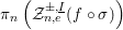 ${\it\pi}_{n}\left({\mathcal{Z}}_{n,e}^{\pm ,\underline{I}}(f\circ {\it\sigma})\right)$ is the globally invariant set
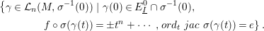 $$\begin{eqnarray}\displaystyle & & \displaystyle \left\{{\it\gamma}\in {\mathcal{L}}_{n}(M,{\it\sigma}^{-1}(0))~|~{\it\gamma}(0)\in E_{\underline{I}}^{0}\cap {\it\sigma}^{-1}(0),\right.\nonumber\\ \displaystyle & & \displaystyle \qquad \qquad \left.f\circ {\it\sigma}({\it\gamma}(t))=\pm t^{n}+\cdots \,,ord_{t}~jac~{\it\sigma}({\it\gamma}(t))=e\right\}.\nonumber\end{eqnarray}$$
 With the same notations as in the proof of Proposition 3.12, let  $k\in A(n,e)$ and let
  ${\it\gamma}\in {\it\pi}_{n}({\mathcal{Z}}_{n,e}^{\pm ,\underline{I}}(f\circ {\it\sigma}))$ such that
  ${\it\gamma}(0)\in E_{I}\cap U_{x}$ and for
  $i\in I$,
  $ord_{t}~{\it\gamma}_{j_{i}}(t)=k_{i}$. The condition
  $f\circ {\it\sigma}({\it\gamma}(t))=\pm t^{n}+\cdots \,$ can be expressed as
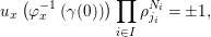 $$\begin{eqnarray}u_{x}\left({\it\varphi}_{x}^{-1}\left({\it\gamma}(0)\right)\right)\mathop{\prod }_{i\in I}{\it\rho}_{j_{i}}^{N_{i}}=\pm 1,\end{eqnarray}$$
 where  ${\it\rho}_{j_{i}}$ is the term of order
  $k_{i}$ in
  ${\it\gamma}_{j_{i}}(t)$. Denote
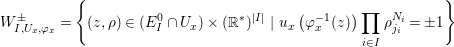 $$\begin{eqnarray}W_{I,U_{x},{\it\varphi}_{x}}^{\pm }=\left\{(z,{\it\rho})\in (E_{I}^{0}\cap U_{x})\times (\mathbb{R}^{\ast })^{|I|}~|~u_{x}\left({\it\varphi}_{x}^{-1}(z)\right)\mathop{\prod }_{i\in I}{\it\rho}_{j_{i}}^{N_{i}}=\pm 1\right\}\end{eqnarray}$$
 and notice that, since for  $g\in G$,
 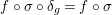 $f\circ {\it\sigma}\circ {\it\delta}_{g}=f\circ {\it\sigma}$, we have
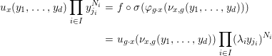 $$\begin{eqnarray}\displaystyle u_{x}(y_{1},\ldots ,y_{d})\mathop{\prod }_{i\in I}y_{j_{i}}^{N_{i}} & = & \displaystyle f\circ {\it\sigma}({\it\varphi}_{g\cdot x}({\it\nu}_{x,g}(y_{1},\ldots ,y_{d})))\nonumber\\ \displaystyle & = & \displaystyle u_{g\cdot x}({\it\nu}_{x,g}(y_{1},\ldots ,y_{d}))\mathop{\prod }_{i\in I}({\it\lambda}_{i}y_{j_{i}})^{N_{i}}\nonumber\\ \displaystyle & & \displaystyle \nonumber\end{eqnarray}$$
 where the constants  ${\it\lambda}_{i}$,
  $i\in I$, are given by the matrix
  $A_{x,g}$. Therefore,
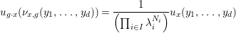 $$\begin{eqnarray}u_{g\cdot x}({\it\nu}_{x,g}(y_{1},\ldots ,y_{d}))=\frac{1}{\left(\mathop{\prod }_{i\in I}{\it\lambda}_{i}^{N_{i}}\right)}u_{x}(y_{1},\ldots ,y_{d})\end{eqnarray}$$
 and in particular, the action of  $g\in G$ on
  $M$ sends
  $W_{I,U_{x},{\it\varphi}_{x}}^{\pm }$ on
  $W_{g\cdot I,U_{g\cdot x},{\it\varphi}_{g\cdot x}}^{\pm }$.
As a consequence, there is an equivariant Nash isomorphism between 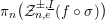 ${\it\pi}_{n}({\mathcal{Z}}_{n,e}^{\pm ,\underline{I}}(f\circ {\it\sigma}))$ and the gluing of the sets
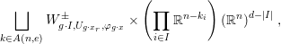 $$\begin{eqnarray}\mathop{\sqcup }_{k\in A(n,e)}W_{g\cdot I,U_{g\cdot x_{r}},{\it\varphi}_{g\cdot x}}^{\pm }\times \left(\mathop{\prod }_{i\in I}\mathbb{R}^{n-k_{i}}\right)\left(\mathbb{R}^{n}\right)^{d-|I|},\end{eqnarray}$$
 along the spaces  $E_{g\cdot I}^{0}\cap U_{g\cdot x_{r}}$,
  $g\in G$,
  $r=1,\ldots ,m$.
Thanks to the additivity of the equivariant virtual Poincaré series and Lemma 3.9, we are then reduced to compute the equivariant virtual Poincaré series of the orbit of the set  $W_{I,U_{x},{\it\varphi}_{x}}^{\pm }$ (notice that, for
  $g_{1},g_{2}\in G$, the sets
  $(E_{g_{1}\cdot I}^{0}\cap U_{g_{1}\cdot x})$ and
  $(E_{g_{2}\cdot I}^{0}\cap U_{g_{2}\cdot x})$ are equal or do not intersect).
Now, consider the isomorphism from  $W_{I,U_{x},{\it\varphi}_{x}}^{\pm }$ to
  $R_{I,U_{x},{\it\varphi}_{x}}^{\pm }\times (\mathbb{R}^{\ast })^{|I|-1}$ given in the proof of [Reference Fichou7, Proposition 3.5], with
 $$\begin{eqnarray}R_{I,U_{x},{\it\varphi}_{x}}^{\pm }:=\left\{(z,t)\in E_{I}^{0}\cap U_{x}\times \mathbb{R}~|~t^{m}=\pm \frac{1}{u_{x}\left({\it\varphi}_{x}^{-1}(z)\right)}\right\},\end{eqnarray}$$
 where  $m$ is the greatest common divisor of the
  $N_{i}$’s,
  $i\in I$. It is defined using integers
  $n_{i}$,
  $i\in I$ such that
  $\sum _{i\in I}n_{i}N_{i}=m$.
These isomorphisms are compatible with the action of  $g\in G$ sending the element
  $(z,t,{\it\kappa})$ of
  $R_{I,U_{x},{\it\varphi}_{x}}^{\pm }\times (\mathbb{R}^{\ast })^{|I|-1}$ to
  $({\it\delta}_{g}(z),\frac{t}{\prod _{i\in I}{\it\lambda}_{i}^{N_{i}/m}},g\cdot {\it\kappa})\in R_{g\cdot I,U_{g\cdot x},{\it\varphi}_{g\cdot x}}^{\pm }\times (\mathbb{R}^{\ast })^{|I|-1}$, the
  $j\text{th}$ coordinate of
  ${\it\kappa}$ being sent to itself times
  $(\prod _{i\in I}{\it\lambda}_{i}^{N_{i}/m})^{-n_{j}}{\it\lambda}_{j}$.
Consequently, the equivariant virtual Poincaré series of the orbit of the set  $W_{I,U_{x},{\it\varphi}_{x}}^{\pm }$ is, using Lemma 3.9,
  $(u-1)^{|I|-1}$ times the equivariant virtual Poincaré series of the orbit of the set
  $R_{I,U_{x},{\it\varphi}_{x}}^{\pm }$.
Thus,
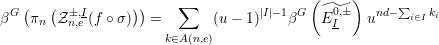 $$\begin{eqnarray}{\it\beta}^{G}\left({\it\pi}_{n}\left({\mathcal{Z}}_{n,e}^{\pm ,\underline{I}}(f\circ {\it\sigma})\right)\right)=\mathop{\sum }_{k\in A(n,e)}(u-1)^{|I|-1}{\it\beta}^{G}\left(\widetilde{E_{\underline{I}}^{0,\pm }}\right)u^{nd-\mathop{\sum }_{i\in I}k_{i}}\end{eqnarray}$$
 where  $\widetilde{E_{\underline{I}}^{0,\pm }}$ is the gluing of the sets
  $R_{g\cdot I,U_{g\cdot x_{r}},{\it\varphi}_{g\cdot x_{r}}}^{\pm }$ along the spaces
  $E_{g\cdot I}^{0}\cap U_{g\cdot x_{r}}$,
  $g\in G$,
  $r=1,\ldots ,m$.
Now, the end of the computation is the same as in step (v) of the proof of Proposition 3.12 (notice that in the above arguments, we dropped the intersection with  ${\it\sigma}^{-1}(0)$ for the sake of readability).◻
Remark 3.19. We can also define the naive equivariant zeta function of the germ of an equivariant Nash function  $f:(\mathbb{R}^{d},0)\rightarrow (\mathbb{R},0)$ where the affine spaces
  $\mathbb{R}^{d}$ and
  $\mathbb{R}$ are both equipped with a linear action of
  $G$. Indeed, if
  $g\mapsto {\it\kappa}_{g}$ denotes the linear action of
  $G$ on
  $\mathbb{R}$, then, since
  $G$ is finite, for all
  $g\in G$,
  ${\it\kappa}_{g}=\pm \text{Id}_{\mathbb{R}}$. Therefore, the spaces of arcs
  $A_{n}(f)$ of
  $f$ are globally stable under the action of
  $G$ on
  ${\mathcal{L}}$. Furthermore, Denef–Loeser formula of Proposition 3.12 is also valid for the naive equivariant zeta function of
  $f$.
$f$.
In order to define equivariant zeta functions with signs for  $f$, we have to consider the kernel
  $H$ of the group morphism
  $g\mapsto {\it\kappa}_{g}$. Then the arc spaces
  $A_{n}^{+}(f)$ and
  $A_{n}^{-}(f)$ are globally stable under the restricted action of
  $H$ on
  ${\mathcal{L}}$ and we can define the equivariant zeta functions with signs of
  $f$ with respect to
  $H$, for which we have Denef–Loeser formula (Proposition 3.17).
We can also consider, for all  $n\geqslant 1$, the equivariant virtual Poincaré series of the reunion of
  $A_{n}^{+}(f)$ and
  $A_{n}^{-}(f)$, which is a
  $G$-
$G$- ${\mathcal{A}}{\mathcal{S}}$-set, and gather this data into a new zeta function. In a subsequent work, we will study this zeta function, as well as its relation to the other equivariant zeta functions of such an equivariant Nash germ
  $f$.
$f$.
4 Equivariant zeta functions and equivariant blow-Nash equivalence
Denef–Loeser formulas for the equivariant zeta functions allow us to show that these latter are invariants for equivariant blow-Nash equivalence via equivariant blow-Nash isomorphisms:
Theorem 4.1. Let  $\mathbb{R}^{d}$ be equipped with a linear action of
  $G$ and let
  $f$,
$f$,  $h:(\mathbb{R}^{d},0)\rightarrow (\mathbb{R},0)$ be two invariant Nash germs. If
  $f$ and
  $h$ are
  $G$-blow-Nash equivalent via an equivariant blow-Nash isomorphism, then
 $$\begin{eqnarray}Z_{f}^{G}(u,T)=Z_{h}^{G}(u,T)\qquad \text{and}\qquad Z_{f}^{G,\pm }(u,T)=Z_{h}^{G,\pm }(u,T).\end{eqnarray}$$
Proof. Let us keep the notations of the definition 2.1 of  $G$-blow-Nash equivalence.
We then apply Proposition 3.12, respectively Proposition 3.17, to both  $f$ and
  $h$ and the expressions of the naive equivariant zeta functions, respectively equivariant zeta functions with signs, of
  $f$ and
  $h$ given by the Denef–Loeser formula are equal because
∙
${\rm\Phi}$ sends the irreducible components of $(f\circ {\it\sigma}_{f})^{-1}(0)$ onto the irreducible components of $(h\circ {\it\sigma}_{h})^{-1}(0)$;∙ the equivariant virtual Poincaré series is invariant under equivariant Nash isomorphisms;
∙ the multiplicities
$N$ are preserved by ${\rm\Phi}$ thanks to the commutativity of the diagram defining $G$-blow-Nash equivalence (see Definition 2.1), and the multiplicities ${\it\nu}$ are preserved by ${\rm\Phi}$ because it is an equivariant blow-Nash isomorphism.◻


Example 4.2. Consider the affine plane  $\mathbb{R}^{2}$ with coordinates
  $(x,y)$, equipped with the
  $\mathbb{Z}/2\mathbb{Z}$-action
  $(x,y)\mapsto (-x,y)$. Let
  $f$ and
  $h$ be the Nash germs at
  $(0,0)$ defined by
 $$\begin{eqnarray}f(x,y)=y^{4}-x^{2};\qquad h(x,y)=x^{4}-y^{2}.\end{eqnarray}$$
 They are Nash equivalent via the Nash isomorphism  ${\rm\Phi}:\mathbb{R}^{2}\rightarrow \mathbb{R}^{2};(x,y)\mapsto (y,x)$. In particular, they are blow-Nash equivalent via a blow-Nash isomorphism and consequently
 $$\begin{eqnarray}Z_{f}(u,T)=Z_{h}(u,T)\end{eqnarray}$$
(the zeta functions are invariants for blow-Nash equivalence via blow-Nash isomorphisms: see [Reference Fichou8]).
However, notice that  ${\rm\Phi}$ is not equivariant with respect to the considered action of
  $G:=\mathbb{Z}/2\mathbb{Z}$ on
  $\mathbb{R}^{2}$. We compute the naive equivariant zeta functions of the invariant Nash germs
  $f$ and
  $h$ and show that they are not
  $G$-blow-Nash equivalent via an equivariant blow-Nash isomorphism, using Theorem 4.1.
Let  ${\it\sigma}_{1}$ be the equivariant blowing-up of
  $\mathbb{R}^{2}$ at the origin and let
  $(\mathbb{R}^{2},(X,Y))$ be the chart of the blowing-up in which
  ${\it\sigma}_{1}$ is given by
  ${\it\sigma}_{1}(X,Y)=(XY,Y)$, the action of
  $G$ on this chart being given by
 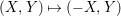 $(X,Y)\mapsto (-X,Y)$. In this chart, we have
  $f\circ {\it\sigma}_{1}(X,Y)=Y^{2}(Y^{2}-X^{2})$.
By a second equivariant blowing-up  ${\it\sigma}_{2}$ given by
  ${\it\sigma}_{2}(W,Z)=(W,WZ)$ in the chart
  $(\mathbb{R}^{2},(W,Z))$, we obtain a function with only normal crossings
 $$\begin{eqnarray}f\circ {\it\sigma}(W,Z)=W^{4}Z^{2}(Z-1)(Z+1),\end{eqnarray}$$
 with  ${\it\sigma}:={\it\sigma}_{1}\circ {\it\sigma}_{2}$. It is in particular invariant under the action of
  $G$ on the chart, given by
  $(W,Z)\mapsto (-W,-Z)$.
The fiber  $f\circ {\it\sigma}^{-1}(0)$ have four irreducible components, given in the chart
  $(\mathbb{R}^{2},(W,Z))$ by
 $$\begin{eqnarray}E_{1}=\{Z=0\},\qquad E_{2}=\{W=0\},\qquad E_{3}=\{Z=1\},\qquad E_{4}=\{Z=-1\}.\end{eqnarray}$$
 The exceptional divisors  $E_{1}$ and
  $E_{2}$, both isomorphic to a circle, intersect at a
  $G$-fixed point and
  $E_{2}$ intersects the irreducible components
  $E_{3}$ and
  $E_{4}$ of the strict transform of
  $f$ at two points exchanged by the action.
Therefore, using the equivariant Denef–Loeser formula, since  $N_{1}=2$,
  ${\it\nu}_{1}=1$,
  $N_{2}=4$,
  ${\it\nu}_{2}=2$ and
  $N_{3}=N_{4}=1$,
  ${\it\nu}_{3}={\it\nu}_{4}=0$, we have after computation (use Example 3.7)
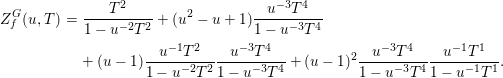 $$\begin{eqnarray}\displaystyle Z_{f}^{G}(u,T) & = & \displaystyle \frac{T^{2}}{1-u^{-2}T^{2}}+(u^{2}-u+1)\frac{u^{-3}T^{4}}{1-u^{-3}T^{4}}\nonumber\\ \displaystyle & & \displaystyle +\,(u-1)\frac{u^{-1}T^{2}}{1-u^{-2}T^{2}}\frac{u^{-3}T^{4}}{1-u^{-3}T^{4}}\hspace{-0.3pt}+\hspace{-0.3pt}(u-1)^{2}\frac{u^{-3}T^{4}}{1-u^{-3}T^{4}}\frac{u^{-1}T^{1}}{1-u^{-1}T^{1}}.\nonumber\end{eqnarray}$$
 In order to compute the naive equivariant zeta function of  $h$, we consider the equivariant blowings-up
  ${\it\sigma}_{1}$ and
  ${\it\sigma}_{2}$ in the respective charts
  $(\mathbb{R}^{2},(U,T))$ and
  $(\mathbb{R}^{2},(R,S))$, where they are given by
  ${\it\sigma}_{1}(U,T)=(U,UT)$ and
  ${\it\sigma}_{2}(R,S)=(RS,S)$. The actions of
  $G$ on these charts are given by
  $(U,T)\mapsto (-U,-T)$ and
  $(R,S)\mapsto (R,-S)$, and we have
 $$\begin{eqnarray}h\circ {\it\sigma}(R,S)=S^{4}R^{2}(R-1)(R+1)\end{eqnarray}$$
 in the chart  $(\mathbb{R}^{2},(R,S))$.
The four irreducible components of  $(h\circ {\it\sigma})^{-1}(0)$ are given by
 $$\begin{eqnarray}E_{1}^{\prime }=\{R=0\},~E_{2}^{\prime }=\{S=0\},~E_{3}^{\prime }=\{R=1\},~E_{4}^{\prime }=\{R=-1\}\end{eqnarray}$$
 and the exceptional divisor  $E_{2}^{\prime }$ intersects the strict transform of
  $h$ at two points that are both fixed by the action of
  $G$. Thus,
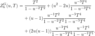 $$\begin{eqnarray}\displaystyle Z_{h}^{G}(u,T) & = & \displaystyle \frac{T^{2}}{1-u^{-2}T^{2}}+(u^{2}-2u)\frac{u^{-3}T^{4}}{1-u^{-3}T^{4}}\nonumber\\ \displaystyle & & \displaystyle +\,(u-1)\frac{u^{-1}T^{2}}{1-u^{-2}T^{2}}\frac{u^{-3}T^{4}}{1-u^{-3}T^{4}}\nonumber\\ \displaystyle & & \displaystyle +\,(2u(u-1))\frac{u^{-3}T^{4}}{1-u^{-3}T^{4}}\frac{u^{-1}T^{1}}{1-u^{-1}T^{1}}.\nonumber\end{eqnarray}$$
In particular,
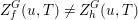 $$\begin{eqnarray}Z_{f}^{G}(u,T)\neq Z_{h}^{G}(u,T)\end{eqnarray}$$
 and therefore, with respect to the considered  $\mathbb{Z}/2\mathbb{Z}$-action on
  $\mathbb{R}^{2}$,
  $f$ and
  $h$ are not
  $G$-blow-Nash equivalent via an equivariant blow-Nash isomorphism, by Theorem 4.1.
5 Examples
In this section, we compute the equivariant zeta functions of several invariant Nash germs under linear actions of  $G:=\mathbb{Z}/2\mathbb{Z}$, using Denef–Loeser formula (Propositions 3.12 and 3.17).
Example 5.1. (See also [Reference Fichou7, Example 3.6])
Equip the affine plane  $\mathbb{R}^{2}$ with any involution of the type
  $s:(x,y)\mapsto ({\it\epsilon}x,{\it\epsilon}^{\prime }y)$ with
  ${\it\epsilon},{\it\epsilon}^{\prime }\in \{-1,1\}$
∙ Consider the invariant Nash germ
$f:(x,y)\mapsto x^{2}+y^{2}$ at $(0,0)$. The equivariant blowing-up of the plane at the origin gives an equivariant resolution ${\it\sigma}$ of the singularities of $f$ and the fiber $(f\circ {\it\sigma})^{-1}(0)$ consists just in the exceptional divisor $E_{1}$ of the blowing-up equipped with the induced nonfree action of $G$, and we obtain (see Example 3.7) Now, since$$\begin{eqnarray}Z_{f}^{G}(u,T)=(u-1)\left(u+2\frac{u}{u-1}\right)\frac{u^{-2}T^{2}}{1-u^{-2}T^{2}}=(u^{2}+u)\frac{u^{-2}T^{2}}{1-u^{-2}T^{2}}.\end{eqnarray}$$$f$ is a positive function, we know that $Z_{f}^{G,-}(u,T)=0$, and, since $\widetilde{E_{\{1\}}^{0,+}}$ is the boundary of a Möbius band equipped with a nonfree action of $G$, $$\begin{eqnarray}Z_{f}^{G,+}(u,T)=\left(u+2\frac{u}{u-1}\right)\frac{u^{-2}T^{2}}{1-u^{-2}T^{2}}.\end{eqnarray}$$∙ Consider the invariant Nash germ
$h:(x,y)\mapsto -x^{2}-y^{4}$. Two successive equivariant blowings-up provide an equivariant resolution of singularities ${\it\tau}$ of $h$. The two exceptional divisors $E_{1}^{\prime }$ and $E_{2}^{\prime }$, intersecting at one $G$-fixed point, constitute the fiber $(h\circ {\it\tau})^{-1}(0)$ and we have The sets$$\begin{eqnarray}\displaystyle Z_{h}^{G}(u,T) & = & \displaystyle u^{2}\frac{u^{-2}T^{2}}{1-u^{-2}T^{2}}+u^{2}\frac{u^{-3}T^{4}}{1-u^{-3}T^{4}}\nonumber\\ \displaystyle & & \displaystyle +\,(u-1)u\frac{u^{-2}T^{2}}{1-u^{-2}T^{2}}\frac{u^{-3}T^{4}}{1-u^{-3}T^{4}}.\nonumber\end{eqnarray}$$$\widetilde{E_{\{1\}}^{0,+}}$ and $\widetilde{E_{\{2\}}^{0,+}}$ are both the boundary of a Möbius band minus two points fixed under the induced action of $G$. Consequently, ($$\begin{eqnarray}Z_{h}^{G,-}(u,T)=u\frac{u^{-2}T^{2}}{1-u^{-2}T^{2}}+u\frac{u^{-3}T^{4}}{1-u^{-3}T^{4}}+2u\frac{u^{-2}T^{2}}{1-u^{-2}T^{2}}\frac{u^{-3}T^{4}}{1-u^{-3}T^{4}}\end{eqnarray}$$$Z_{h}^{G,+}(u,T)=0$ since $h$ is negative).
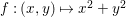


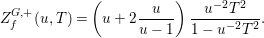
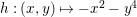


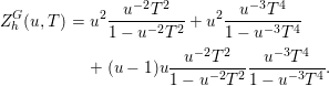


In Example 5.2 below, the affine plane  $\mathbb{R}^{2}$ is equipped with the action of
  $G$ given by the involution
  $s:(x,y)\mapsto (-x,y)$. We compute the naive equivariant zeta functions of the invariant Nash germs
  $f$,
$f$,  $g_{k}$,
  $k\geqslant 2$, and
  $h_{k}$,
  $k\geqslant 2$, at the origin of
  $\mathbb{R}^{2}$ given by
 $$\begin{eqnarray}f(x,y)=\pm x^{4}+y^{3};\qquad g_{k}(x,y)=\pm x^{2k}\pm y^{2};\qquad h_{k}(x,y)=x^{2}y\pm y^{k}.\end{eqnarray}$$
These germs are induced from the normal forms of the simple boundary singularities of manifolds with boundary, by unfolding the positive abscissa half-plane along the ordinate axis (see [Reference Arnold, Gusein-Zade and Varchenko1]). We will study the classification of the simple boundary singularities of Nash manifolds with boundary up to (equivariant) blow-Nash equivalence in a subsequent work.
(1) We begin with
$f$. Consider the equivariant blowing-up ${\it\sigma}_{1}$ at the origin given in the chart $(\mathbb{R}^{2},(X_{1},Y_{1}))$ by ${\it\sigma}_{1}(X_{1},Y_{1})=(X_{1},X_{1}Y_{1})$. The action of $G$ on the blowing-up is given in this chart by $s_{1}:(X_{1},Y_{1})\mapsto (-X_{1},-Y_{1})$ and we have $$\begin{eqnarray}f\circ {\it\sigma}_{1}(X_{1},Y_{1})=X_{1}^{3}(Y_{1}^{3}\pm X_{1}).\end{eqnarray}$$We do three more successive blowings-up
${\it\sigma}_{2}$, ${\it\sigma}_{3}$ and ${\it\sigma}_{4}$ each given in the chart $(\mathbb{R}^{2},(X_{i},Y_{i}))$ by ${\it\sigma}_{i}(X_{i},Y_{i})=(X_{i}Y_{i},X_{i})$. The action of $G$ on the last blowing-up is given in the chart $(\mathbb{R}^{2},(X_{4},Y_{4}))$ by $s_{4}:(X_{4},Y_{4})\mapsto (X_{4},-Y_{4})$ and we have where$$\begin{eqnarray}f\circ {\it\sigma}(X_{4},Y_{4})=X_{4}^{3}Y_{4}^{12}(1\pm X_{4})\end{eqnarray}$$${\it\sigma}:={\it\sigma}_{1}\circ \cdots \circ {\it\sigma}_{4}$.The (equivariant) resolution tree of
$f$ is the following, where $E_{i}(N_{i},{\it\nu}_{i})$ denotes the exceptional divisor of the blowing-up ${\it\sigma}_{i}$ with $N_{i}=mult_{E_{i}}~f\circ {\it\sigma}_{i}=mult_{E_{i}}~f\circ {\it\sigma}$ and ${\it\nu}_{i}=1+mult_{E_{i}}~jac~{\it\sigma}_{i}=1+mult_{E_{i}}~jac~{\it\sigma}$: The sets$$\begin{eqnarray}\displaystyle & & \displaystyle \nonumber\end{eqnarray}$$$E_{-}$ and $E_{+}$ are the respective strict transforms of $f_{-}(x,y)=-x^{3}+y^{4}$ and $f_{+}(x,y)=x^{3}+y^{4}$. In both cases, the action of $G$ globally stabilizes the strict transform, the exceptional divisors and the intersections. Then Denef–Loeser formula provides the naive equivariant zeta function of $f$ (using also Example 3.7): $$\begin{eqnarray}\displaystyle Z_{f}^{G}(u,T) & = & \displaystyle \mathop{\sum }_{i=1}^{3}\frac{u^{-{\it\nu}_{i}+2}T^{N_{i}}}{1-u^{-{\it\nu}_{i}}T^{N_{i}}}+(u-1)\frac{u^{-6}T^{12}}{1-u^{-7}T^{12}}\nonumber\\ \displaystyle & & \displaystyle +\,(u-1)\frac{u^{-2}T^{4}}{1-u^{-3}T^{4}}\frac{u^{-5}T^{8}}{1-u^{-5}T^{8}}+(u-1)\frac{u^{-6}T^{12}}{1-u^{-7}T^{12}}\nonumber\\ \displaystyle & & \displaystyle \times \,\left[\frac{u^{-5}T^{8}}{1-u^{-5}T^{8}}+\frac{u^{-2}T^{3}}{1-u^{-2}T^{3}}+\frac{u^{-1}T^{1}}{1-u^{-1}T^{1}}\right]\nonumber\end{eqnarray}$$(2) We now compute the naive equivariant zeta function of
$g_{k}$ for $k\geqslant 3$. By $k$ successive equivariant blowings-up ${\it\sigma}_{i}$, $i=1,\ldots ,k$, given in charts $(\mathbb{R}^{2},(X_{i},Y_{i}))$ by ${\it\sigma}_{i}:(X_{i},Y_{i})\mapsto (X_{i},X_{i}Y_{i})$, we resolve the singularities of $g_{k}$ : with$$\begin{eqnarray}g_{k}\circ {\it\sigma}(X_{k},Y_{k})=X_{k}^{2k}(\pm 1\pm Y_{k}^{2})\end{eqnarray}$$${\it\sigma}:={\it\sigma}_{1}\circ \cdots \circ {\it\sigma}_{k}$.First, we deal with the case
$g_{k}(x,y)=\pm (x^{2k}-y^{2})$. In this case, we have the following resolution tree for $g_{k}$: $$\begin{eqnarray}\displaystyle & & \displaystyle \nonumber\end{eqnarray}$$In the chart
$(\mathbb{R}^{2},(X_{k},Y_{k}))$, the action of $G$ is given by Thus, the intersection points of the strict transform$$\begin{eqnarray}s_{k}:(X_{k},Y_{k})\mapsto \left\{\begin{array}{@{}ll@{}}(-X_{k},-Y_{k})\quad & \text{if }k\text{ is odd,}\\ (-X_{k},Y_{k})\quad & \text{if }k\text{ is even.}\end{array}\right.\end{eqnarray}$$$E$ of $g_{k}$ with the exceptional divisor $E_{k}$ are exchanged under the involution if $k$ is odd and fixed if $k$ is even.Consequently, after computation we obtain
with$$\begin{eqnarray}\displaystyle Z_{g_{k}}^{G}(u,T) & = & \displaystyle \frac{T^{2}}{1-u^{-2}T^{2}}+(u-1)\left[\mathop{\sum }_{j=2}^{k-1}\frac{u^{-j}T^{2j}}{1-u^{-(j+1)}T^{2j}}\right.\nonumber\\ \displaystyle & & \displaystyle \left.+\,\mathop{\sum }_{j=1}^{k-1}\frac{u^{-j}T^{2j}}{1-u^{-(j+1)}T^{2j}}\frac{u^{-(j+2)}T^{2j+2}}{1-u^{-(j+2)}T^{2j+2}}\right]+{\rm\Lambda}_{k}(u,T)\nonumber\end{eqnarray}$$$$\begin{eqnarray}{\rm\Lambda}_{k}(u,T)=\left\{\begin{array}{@{}l@{}}(u^{2}-u+1){\displaystyle \frac{u^{-(k+1)}T^{2k}}{1-u^{-(k+1)}T^{2k}}}\quad \\ \qquad +\,(u-1)^{2}{\displaystyle \frac{u^{-(k+1)}T^{2k}}{1-u^{-(k+1)}T^{2k}}}{\displaystyle \frac{u^{-1}T^{1}}{1-u^{-1}T^{1}}}\quad \text{if }k\text{ is odd, }\quad \\ (u-2){\displaystyle \frac{u^{-k}T^{2k}}{1-u^{-(k+1)}T^{2k}}}\quad \\ \qquad +\,2u(u-1){\displaystyle \frac{u^{-(k+1)}T^{2k}}{1-u^{-(k+1)}T^{2k}}}{\displaystyle \frac{u^{-1}T^{1}}{1-u^{-1}T^{1}}}\quad \text{if }k\text{ is even.}\quad \end{array}\right.\end{eqnarray}$$In the case
$g_{k}(x,y)=\pm (x^{2k}+y^{2})$, there is no strict transform and the naive equivariant zeta function of $g_{k}$ is given by the same formula as above with $$\begin{eqnarray}{\rm\Lambda}_{k}(u,T)=\frac{u^{-k+1}T^{2k}}{1-u^{-(k+1)}T^{2k}}.\end{eqnarray}$$(3) Let us next consider the invariant Nash germ
$h_{k}$, $k\geqslant 3$. We first look at the case $k$ odd. If $k=2p+1$ with $p\in \mathbb{N}$, then $p$ successive equivariant blowings-up ${\it\sigma}_{i}:(X_{i},Y_{i})\rightarrow (X_{i}Y_{i},Y_{i})$ provide the function with only normal crossings together with the following resolution tree$$\begin{eqnarray}h_{k}\circ {\it\sigma}_{1}\circ \cdots \circ {\it\sigma}_{p}(X_{p},Y_{p})=Y_{p}^{k}(X_{p}^{2}\pm 1),\end{eqnarray}$$(the above resolution tree corresponds to the case$$\begin{eqnarray}\displaystyle & & \displaystyle \nonumber\end{eqnarray}$$$h_{k}(x,y)=x^{2}y-y^{k}$; in the case $h_{k}(x,y)=x^{2}y+y^{k}$, there is no strict transform). In the chart $(\mathbb{R}^{2},(X_{p},Y_{p}))$, the action of $G$ is given by $s_{p}:(X_{p},Y_{p})\mapsto (-X_{p},Y_{p})$, hence exchanges the intersection points of the strict transform $E$ of $h_{k}$ with the exceptional divisor $E_{p}$.If now we suppose
$k=2p$ with $p\in \mathbb{N}\setminus \{0,1\}$, by doing the same first $p-1$ successive equivariant blowings-up ${\it\sigma}_{1},\ldots ,{\it\sigma}_{p-1}$ as above, regarded in the same charts, we obtain $$\begin{eqnarray}h_{k}\circ {\it\sigma}_{1}\circ \cdots \circ {\it\sigma}_{p-1}(X_{p-1},Y_{p-1})=Y_{p-1}^{2p-1}(X_{p-1}^{2}\pm Y_{p-1}).\end{eqnarray}$$We obtain the equivariant resolution of singularities of
$h_{k}$ by two more equivariant blowings-up, getting the following tree: (where$$\begin{eqnarray}\displaystyle & & \displaystyle \nonumber\end{eqnarray}$$$E_{-}$ and $E_{+}$ are the respective strict transforms of $x^{2}y-y^{k}$ and $x^{2}y+y^{k}$), all the intersection points being fixed by the action of $G$.(4) Finally, we take a look at the germs
$g_{2}$ and $h_{2}$. By applying the same two equivariant blowings-up regarded in the same charts, we obtain isomorphic resolution trees for $h_{2}$ and $g_{2}:(x,y)\mapsto \pm (x^{4}-y^{2})$ with same multiplicities, the action of $G$ fixing all intersection points. Notice that the case $g_{2}(x,y)=\pm (x^{4}+y^{2})$ is treated in Example 5.1 up to equivariant Nash equivalence.


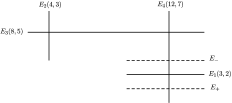


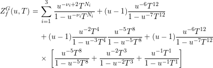


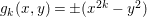

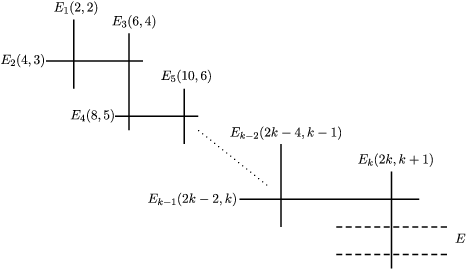


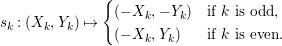


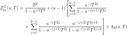
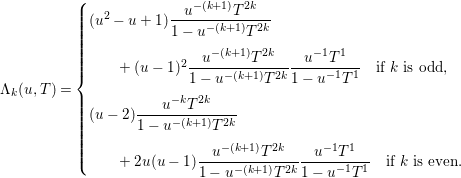
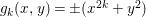

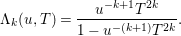


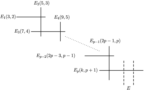


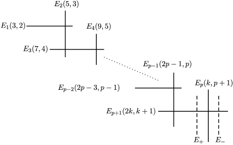


Acknowledgments
The author wishes to thank G. Fichou and T. Fukui for useful discussions and comments.
