


1. Introduction
Particle-laden turbulent flows are multiphase systems where a carrier fluid interacts with a dispersed phase made up by a number of solid objects, e.g. spheres or fibres. Such flows concern an important class of problems with numerous applications related to both natural and industrial processes (De Lillo et al. Reference De Lillo, Cencini, Durham, Barry, Stocker, Climent and Boffetta2014; Breard et al. Reference Breard, Lube, Jones, Dufek, Cronin, Valentine and Moebis2016; Sengupta, Carrara & Stocker Reference Sengupta, Carrara and Stocker2017; Falkinhoff et al. Reference Falkinhoff, Obligado, Bourgoin and Mininni2020; Rosti et al. Reference Rosti, Olivieri, Cavaiola, Seminara and Mazzino2020). In the analysis and modelling of such problems, a crucial distinction can be made regarding the mutual coupling between the carrier flow and the dispersed objects. When the suspension is dilute enough, it can be safely assumed that the fluid flow is not substantially altered by the presence of the objects (Balachandar & Eaton Reference Balachandar and Eaton2010; Maxey Reference Maxey2017; Brandt & Coletti Reference Brandt and Coletti2021).
However, we often deal with non-dilute conditions where the mutual coupling between the two phases is relevant and gives rise to a macroscopic alteration of the turbulent carrier flow. The resulting turbulence modulation effects have been the subject of previous studies over different classes of multiphase turbulent flows, i.e. considering isotropic (Lucci, Ferrante & Elghobashi Reference Lucci, Ferrante and Elghobashi2010; Gualtieri et al. Reference Gualtieri, Picano, Sardina and Casciola2013; Uhlmann & Chouippe Reference Uhlmann and Chouippe2017; Capecelatro, Desjardins & Fox Reference Capecelatro, Desjardins and Fox2018; Ardekani, Rosti & Brandt Reference Ardekani, Rosti and Brandt2019; Yousefi, Ardekani & Brandt Reference Yousefi, Ardekani and Brandt2020) or anisotropic (Andersson, Zhao & Barri Reference Andersson, Zhao and Barri2012; Olivieri et al. Reference Olivieri, Brandt, Rosti and Mazzino2020b,Reference Olivieri, Akoush, Brandt, Rosti and Mazzinoa; Olivieri, Mazzino & Rosti Reference Olivieri, Mazzino and Rosti2021, Reference Olivieri, Mazzino and Rosti2022; Wang et al. Reference Wang, Yi, Jiang and Sun2022) solid particles, as well as droplets or bubbles (Dodd & Ferrante Reference Dodd and Ferrante2016; Freund & Ferrante Reference Freund and Ferrante2019; Rosti et al. Reference Rosti, Ge, Jain, Dodd and Brandt2019; Cannon et al. Reference Cannon, Izbassarov, Tammisola, Brandt and Rosti2021), typically focusing on the alteration of both the bulk flow properties as well as the scale-by-scale energy distribution. In particular, Lucci et al. (Reference Lucci, Ferrante and Elghobashi2010) and Yousefi et al. (Reference Yousefi, Ardekani and Brandt2020) showed that Taylor-length-scale-sized spheres reduce turbulent kinetic energy at the large scales and enhance its energy content at the small scales.
Nevertheless, the accurate characterization of the underlying physics in these complex systems still requires significant efforts from the theoretical, computational and experimental viewpoints, with relevant questions still not fully addressed, such as the following. (i) What are the mechanisms controlling the scale-by-scale energy distribution in the presence of immersed objects with finite size (i.e. larger than the dissipative length scale)? (ii) How do the geometrical properties of the dispersed particles (i.e. their size and isotropy) affect the back-reaction on the carrier flow and the consequent turbulence modulation?
In this work, we comprehensively investigate the multiscale nature of the turbulence modulation due to finite-size rigid particles, focusing on the role of geometrical properties and comparing, in particular, the back-reaction caused by isotropic bluff objects (i.e. spheres) versus anisotropic slender ones (i.e. fibres). Exploiting massive direct numerical simulations (DNS), it is observed, at first, that the macroscopic effect in the turbulence modulation essentially consists of a large-scale energy depletion for both configurations. However, we show that this bulk effect arises from qualitatively different mechanisms depending on the geometrical features of the dispersed objects, which becomes evident from a scale-by-scale energy-transfer balance. For isotropic objects (spheres), the back-reaction effectively acts at a well-defined length scale (i.e. the sphere diameter) and over a limited range of smaller scales, without appreciably modifying the inertial range that is obtained in the single phase (i.e. without particles) configuration. For anisotropic objects (fibres), instead, the fluid–solid coupling is responsible for a global modification of the energy distribution over all the scales of motion, which is characterized by the emergence of an alternative energy flux along with a relative enhancement of small-scale fluctuations.
The rest of the paper is structured as follows: § 2 describes the modelling and computational methodology, § 3 shows the results, and § 4 contains the conclusions.
2. Methods
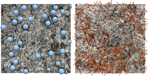
To investigate the problem, we devote our attention to particles of finite size (i.e. diameter or length) that lies well within the inertial subrange of the turbulent flow. A visual example of two representative configurations is given in figure 1. Specifically, we have performed DNS where the fluid and solid dynamics are mutually coupled using the immersed boundary method (Hori, Rosti & Takagi Reference Hori, Rosti and Takagi2022; Olivieri et al. Reference Olivieri, Mazzino and Rosti2022). An incompressible, homogeneous and isotropic turbulent (HIT) flow is generated within a tri-periodic cubic domain of size  $L=2{\rm \pi}$ using Arnold–Beltrami–Childress (ABC) cellular-flow forcing (Podvigina & Pouquet Reference Podvigina and Pouquet1994), achieving in the single-phase case a microscale Reynolds number
  ${Re}_\lambda = u' \lambda / \nu \approx 435$, where
  $u'$ is the root mean square of the turbulent fluctuations,
  $\lambda$ is the Taylor microscale and
  $\nu$ is the kinematic viscosity. Such a high-Reynolds-number configuration is computationally explored for the first time in the framework of multiphase flows in order to achieve proper scale separation. As shown in figure 2, the energy spectrum in the single-phase configuration (black curve) shows the classical Kolmogorov scaling
  ${\sim }\kappa ^{-5/3}$ (dashed line) at low-to-intermediate wavenumbers over more than one decade.

Figure 1. Two-dimensional views of the vorticity magnitude of homogeneous isotropic turbulence in the presence of dispersed, finite-size (a) spheres and (b) fibres, from two representative cases of the present DNS study.

Figure 2. Energy spectra of the modulated turbulent flow for (a) spheres and (b) fibres, for different mass fractions  $M$ (increasing with the colour brightness from dark to light), along with the reference single-phase configuration (i.e.
  $M=0$, black curve) and the expected Kolmogorov scaling in the inertial subrange (grey dashed line). The insets report the microscale Reynolds number
  ${Re}_\lambda$ as a function of the mass fraction; error bars show the standard deviation in
  ${Re}_\lambda$ from the time-averaged value. As an additional check on the accuracy of the computations, diamonds show results calculated using an Eulerian grid with halved resolution (
 $512^{3}$ cells), which produces little change in
  ${Re}_\lambda$ and the inertial range of the spectra.
Once the single-phase case has reached the fully developed regime,  $N$ rigid spheres (characterized by diameter
  $D$ and volumetric density
  $\rho _{s}$) or fibres (characterized by length
  $c$ and linear density difference
  $\Delta \tilde {\rho }_{s}$) are added to the carrier flow at randomly initialized positions and orientations. The multiphase cases were therefore evolved until reaching a statistically stationary state. An overview of the main configurations considered in our study is shown in table 1.
Table 1. Parametric combinations investigated in our baseline study. Left: Suspensions of bluff, spherical particles ( $\rho _{s}$ is the volumetric density of the solid phase, and
  $D$ is the sphere diameter). Right: Suspensions of anisotropic, slender particles (
 $\Delta \tilde {\rho }$ is the linear density difference between the solid and fluid phases, and
  $c$ is the fibre length). Here,
  $\eta$ is the Kolmogorov microscale of the single-phase case,
  ${St}$ is the estimated Stokes number of the particle,
  $N$ is the number of dispersed particles,
  $M$ is the corresponding mass fraction, and
  ${Re}_\lambda$ and
  $C_d$ are the resulting microscale Reynolds number and drag coefficient of the modulated flow, respectively (for
  $M=0$,
  ${Re}_\lambda \approx 435$ and
  $C_d \approx 0.12$). The cases with
  $\rho _{s}=\infty$ and
  $\Delta \tilde {\rho }=\infty$ correspond to the configurations where the particles are retained fixed. In addition to the cases reported in the table, we have performed another set of simulations in the fixed-particle arrangement varying
  $N$ and
  $D$ or
  $c$ (the results of which are reported in figure 5).

The dynamics of the bluff, spherical objects is governed by the well-known Newton–Euler equations (Hori et al. Reference Hori, Rosti and Takagi2022), whereas the slender, anisotropic ones are modelled in the general framework of the Euler–Bernoulli equation for inextensible filaments, choosing a sufficiently large bending stiffness such that the deformation is always negligible (i.e. within 1 %) (Cavaiola, Olivieri & Mazzino Reference Cavaiola, Olivieri and Mazzino2020; Brizzolara et al. Reference Brizzolara, Rosti, Olivieri, Brandt, Holzner and Mazzino2021). Hence, the mass fraction  $M$ of the suspension is defined as the ratio between the mass of the dispersed solid phase and the total mass (i.e. the sum of the fluid and solid masses contained in the domain). Note that for the chosen parameters and when matching
  $M$, bluff and slender particles have remarkably different Stokes numbers, here computed using expressions for small particles, i.e. of length below the dissipative scale, for the sake of a comparative estimate (Lucci, Ferrante & Elghobashi Reference Lucci, Ferrante and Elghobashi2011; Bounoua, Bouchet & Verhille Reference Bounoua, Bouchet and Verhille2018). Moreover, we indicate
  $M=1$ as the configurations where the dispersed objects are constrained to a fixed random position; such a setting serves as the limiting case where the dispersed phase has infinitely large inertia, as well as a representation of flows in porous media. Finally, we note that sphere and fibre cases with the same mass fractions have different volume fractions but approximately the same total wetted area.
To solve the governing equations numerically, we employ the in-house solver Fujin (https://groups.oist.jp/cffu/code). The code is based on the (second-order) central finite-difference method for the spatial discretization and the (second-order) Adams–Bashforth scheme for the temporal discretization. The incompressible Navier– Stokes equations are solved using the fractional step method on a staggered grid. The Poisson equation enforcing the incompressibility constraint is solved using a fast and efficient approach based on the fast Fourier transform (FFT). The solver is parallelized using the MPI protocol and the 2decomp library for domain decomposition (http://www.2decomp.org). In this work, the fluid domain is discretized onto a uniform Eulerian grid using  $1024^{3}$ cells, ensuring that, for the chosen set of domain size and fluid properties, the ratio between the Kolmogorov dissipative length scale and the grid spacing is
  $\eta /\Delta x = {O}(1)$. The carrier- and dispersed-phase dynamics are coupled by the no-slip condition
  $\dot {\boldsymbol {X}} = \boldsymbol {U} = \boldsymbol {u} ( \boldsymbol {X},t )$, where
  $\boldsymbol {X}$ is the position of a generic material point on the solid surface and
  $\boldsymbol {u}=\boldsymbol {u}( \boldsymbol {x},t )$ is the fluid velocity field. In the present work, we employ two types of immersed boundary (IB) method where the mutual interaction between the two phases is achieved by means of a singular force distribution. Specifically, for bluff spherical particles we use the Eulerian IB method recently proposed by Hori et al. (Reference Hori, Rosti and Takagi2022), whereas for slender fibres we use the method originally proposed by Huang, Shin & Sung (Reference Huang, Shin and Sung2007) and recently employed for fibre-laden turbulence by Olivieri et al. (Reference Olivieri, Akoush, Brandt, Rosti and Mazzino2020a,Reference Olivieri, Brandt, Rosti and Mazzinob, Reference Olivieri, Mazzino and Rosti2021, Reference Olivieri, Mazzino and Rosti2022). Overall, the code has been extensively validated and tested in a variety of problems; see e.g. Rosti & Brandt (Reference Rosti and Brandt2020), Rosti et al. (Reference Rosti, Olivieri, Cavaiola, Seminara and Mazzino2020, Reference Rosti, Cavaiola, Olivieri, Seminara and Mazzino2021) and Olivieri et al. (Reference Olivieri, Mazzino and Rosti2022).
3. Results
3.1. Main features of turbulence modulation
The presence of the dispersed phase clearly causes a complex modification of the key features of the carrier flow, as may be observed in the energy spectra for suspensions of spheres (figure 2a) or fibres (figure 2b) at different mass fractions  $M$. At first glance, and focusing on the smallest wavenumbers (i.e. largest scales), one can note a similar phenomenology between the two kinds of particles, with an overall tendency to decrease the turbulent kinetic energy while increasing
  $M$. Indeed, for both bluff and slender particles, the energy-containing scales are depleted by the hydrodynamic drag exerted by the particles. A direct indication on how the bulk properties of the flow are altered is provided in the insets of figure 2, showing a very similar variation between spheres and fibres in terms of
  ${Re}_\lambda$ with the mass fraction, notwithstanding the different Stokes numbers of the suspended objects, in agreement with previous findings (Hwang & Eaton Reference Hwang and Eaton2006; Olivieri et al. Reference Olivieri, Mazzino and Rosti2021, Reference Olivieri, Mazzino and Rosti2022).
However, from figure 2 some peculiar differences between the two kinds of suspensions can also be noticed when extending the observation to the full range of active scales. For bluff particles, the alteration of the energy spectrum with  $M$ remains almost entirely limited to the low-wavenumber region (i.e.
  $\kappa \lesssim 5$), with only a minimal increase at the largest wavenumbers (i.e.
  $\kappa \gtrsim 300$) associated with the high-shear regions in the boundary layers around the spheres. Instead, for fibres, the modulation extends up to the highest wavenumber (i.e.
  $\kappa _{max} = 512$). At sufficiently large
  $M$, a departure from the Kolmogorov scaling indeed appears throughout the full inertial subrange. We anticipate that here the energy transfer is mainly due to the fluid–solid coupling, and not to the convective term as in the single-phase or bluff particle cases, leading to a different form of energy flux.
A quantitative evaluation of the resulting power law  $E(\kappa ) \sim \kappa ^{-\beta }$ in the inertial subrange of both single-phase and multiphase flows is given in figure 3, showing the scaling exponent
  $\beta$ as a function of the mass fraction for both spheres and fibres. The single-phase flow (
 $M=0$) and the flows with spheres can be seen to follow the Kolmogorov scaling (
 $\beta =5/3$), whereas the flows with fibres show a significant reduction in
  $\beta$ as
  $M$ increases. An heuristic explanation for the latter trend is that fibres act as a barrier to the flow between any two points with separation greater than the fibre diameter
  $d$, which influences the scaling of the second-order velocity structure function
  $\langle (\delta u)^{2} \rangle \sim r^{\gamma }$ for two points at a distance
  $r > d$, with
  $\gamma = \beta - 1$. In the single-phase case
  $\gamma = 2/3$, whereas the presence of fibres tends to decorrelate the flow, thus reducing the value of
  $\gamma$ or, equivalently,
  $\beta$.

Figure 3. Dependence of the exponent  $\beta$ in the energy spectrum scaling
  $E\sim \kappa ^{-\beta }$ on particle mass fraction
  $M$. Flows with spheres are marked in blue, flows with fibres in orange, and the single-phase flow in black. The blue and orange shaded regions show the approximate error in
  $\beta$, estimated by moving the time averaging window. The Kolmogorov scaling is marked by a grey dotted line.
3.2. Scale-by-scale energy transfer
A clear distinction in the mechanism of energy distribution between the two geometrical configurations can be highlighted. To gain a more detailed insight, we look at the scale-by-scale energy transfer balance
 \begin{equation} \mathcal{P}(\kappa) + \varPi (\kappa) + \varPi_{fs}(\kappa) + \mathcal{D}(\kappa) = \epsilon, \end{equation}
where  $\mathcal {P}$ is the turbulence production associated with the external forcing (acting only at the largest scale
  $\kappa =1$),
  $\varPi$ and
  $\varPi _{fs}$ are the energy fluxes associated with the nonlinear convective term and the fluid–solid coupling term, respectively, and
  $\mathcal {D}$ is the viscous dissipation (Olivieri et al. Reference Olivieri, Mazzino and Rosti2021, Reference Olivieri, Mazzino and Rosti2022).
In figure 4, we show the energy fluxes and dissipation in two representative cases with strong back-reaction ( $M=0.9$) for (a) bluff objects and (b) slender particles. Focusing on the two different energy fluxes (i.e.
  $\varPi$ and
  $\varPi _{fs}$), we note at first that the sum of these two contributions (thin dotted line) appears in both cases as a horizontal plateau for relatively low wavenumbers, as expected from (3.1) and similar to the single-phase case. However, qualitatively different scenarios can be identified for bluff versus slender objects when analysing the two distinct contributions separately. On the other hand, it can be noticed that in both cases, and similarly to the classical, single-phase case, for sufficiently large wavenumbers the energy fluxes tend to zero, and the viscous dissipation
  $\mathcal {D}$ recovers the totality of the balance.

Figure 4. Scale-by-scale energy transfer balance for two representative configurations at  $M=0.9$ of (a) spheres and (b) fibres, showing the contributions of fluid–solid coupling
  $\varPi _{fs}$ (solid line), nonlinear convection
  $\varPi$ (dashed line) and viscous dissipation
  $\mathcal {D}$ (dash-dotted line), each normalized with the average dissipation rate
  $\epsilon$. Furthermore, the total energy flux,
  $\varPi _{fs} + \varPi$, is also reported (dotted line).
For bluff objects (figure 4a), we first have a dominance of the fluid–solid coupling contribution  $\varPi _{fs}$ within a limited low-wavenumber range, and only subsequently of the convective term
  $\varPi$ for larger
  $\kappa$. Indeed, two distinct plateau-like regions are found over two distinct subranges of scales, suggesting that, for increasing
  $\kappa$, the energy is first transferred from the largest scales (where energy is injected) to smaller ones mainly by the action of the particles, only after which the nonlinear term prevails and the balance substantially recovers the classical energy cascade predicted by Kolmogorov theory.
For slender objects (figure 4b), the scenario looks radically different, with  $\varPi _{fs}$ acting over a much wider range of scales and being responsible for transferring most of the energy across all scales, with the nonlinear term being weakened overall. It should also be noted that such alternative energy flux is overall prolonged with respect to the single-phase case, consistent with the observed alteration in the energy spectrum (figure 2b). Note that we refer to an energy flux also for fibre-laden turbulence, because not only is
  $\varPi _{fs}$ constant across a wide range of scales, but also the overall drag coefficient
  $C_d = \epsilon / (u'^{3} \kappa _{in})$ here
  $\kappa _{in}=1$ is the wavenumber at which the energy is injected (Alexakis & Biferale Reference Alexakis and Biferale2018), remains finite and comparable with the single-phase case (see ).
3.3. Characteristic length scale of the fluid–solid coupling
The reason for the observed difference between bluff and slender objects can be ascribed indeed to specific geometrical features. For bluff, isotropic particles the most representative scale is uniquely identified as the particle diameter  $D$. For slender fibres, the back-reaction could be expected instead to act across multiple length scales, approximately ranging from the fibre length
  $c$ to the cross-sectional diameter
  $d$. In fact, the latter is found to have the dominant role (as later shown in figure 5). This qualitative difference has a remarkable consequence on the properties of the modulated turbulent flow at sufficiently small scales: on the one hand, spherical particles affect the flow essentially only at a scale that is well within the inertial range, without modifying the extension and energy amplitude of the latter; on the other hand, slender fibres are directly acting on wavenumbers that are also beyond the original energy cascade.

Figure 5. Fluid–solid coupling contribution to the energy-spectrum balance for (a) spheres and (b) fibres for various mass fractions  $M$ (varying with colour brightness). Circles are plotted for the cases with (a) smaller diameter
  $D$ or (b) shorter length
  $c$, while different line styles are used to denote the variation of the number of objects
  $N$. For ease of comparison, the
  $y$-axis is normalized by the maximum value of the reported quantity. The inset in (a) shows the same data as a function of the wavenumber
  $\kappa$ normalized with the sphere diameter
  $D$. Images show wakes that are similar in size to the (a) sphere diameter and (b) fibre diameter.
To isolate the characteristic length scale up to which the energy is transferred by the back-reaction for the two kinds of dispersed objects, we show in figure 5 the fluid–solid coupling contribution in the energy-spectrum balance, i.e.  $F_{fs}$, such that
  $\int _\kappa ^{\infty } F_{fs} = \varPi _{fs}$. To this aim, along with the variation of the mass fraction, we also consider the influence of the sphere diameter
  $D$ or fibre length
  $c$ in the limiting case of fixed objects (or infinite inertia). For bluff (isotropic) objects (figure 5a), it can be clearly observed that the peak of
  $F_{fs}$ scales with the diameter
  $D$, as also shown from the inset, where the wavenumber is normalized using such quantity. For slender (anisotropic) objects (figure 5b), we observe instead that the fibre length
  $c$ does not appreciably change the position of the peak of
  $F_{fs}$; rather, it appears to be controlled by the fibre diameter
  $d$. Differently from spheres, here the fluid–solid contribution shows a wider distribution, therefore suggesting a quantitative role of the fibre length as well, as previously suggested. For both objects, the mass fraction appears to control not the wavenumber associated with the maximum forcing but only the strength of the back-reaction. Remarkably, the same holds also when varying the number of objects
  $N$.
$N$.
3.4. Phenomenological interpretation
A simple and effective interpretation of our results can be proposed by considering the characteristic Reynolds number experienced by the particles, i.e.  ${Re}_\ell = u' \ell /\nu$, in order to argue the main hydrodynamic effect caused by the solid objects and discern peculiar differences between bluff and slender objects. For the sake of simplicity, we consider the root mean square of the fluid velocity fluctuations
  $u'$ (accounting for its variation due to the effective back-reaction) and the sphere diameter
  $D$ or the fibre diameter
  $d$ as the reference length scale
  $\ell$. For the spherical particles such a choice is natural, whilst for fibres it comes from that previously observed for the energy-transfer balance (figure 5b).
When computing the characteristic Reynolds number, we typically find that for spheres  ${Re}_D \sim {O}(10^{3})$, whereas for fibres
  ${Re}_d \sim {O}(10^{1})$. These estimates suggest that bluff and slender objects experience qualitatively different hydrodynamic regimes, one dominated by inertial and the other by viscous forces, respectively. In particular, spheres are subject to a large-Reynolds-number flow, inducing a turbulent wake on scales comparable with and smaller than
  $D$, while fibres generate flow structures typical of laminar vortex shedding on scales comparable with
  $d$, but without any further proliferation of scales due to the dominant viscous dissipation. Note that here we refer to the range of scales smaller than the characteristic length scale associated with the individual particles. For spheres, the energy of the generated wakes is therefore converted into smaller structures by means of the well-known energy cascading process (controlled by the nonlinear term
  $\varPi$); for fibres, a similar phenomenology is not possible since the smaller-scale generated flow structures are essentially within the dissipative region.
3.5. On the intermittency of the modulated turbulence
Strong spatial and/or temporal fluctuations in the energy flux are the source of intermittency in turbulent flows. Owing to the different nature of the flux in the two configurations, it is natural to wonder how intermittency is altered. A comprehensive approach to study this is to compute the multifractal spectrum of the energy dissipation rate (Sreenivasan & Meneveau Reference Sreenivasan and Meneveau1988), which we report in figure 6. For spheres, we find that  $F(\alpha )$ is substantially similar to the single-phase case with only minor differences. On the other hand, for fibres, we have a remarkable qualitative difference in the spectrum. This further supports the idea of a standard energy cascade in particle-laden flows with finite-size spherical particles, whilst it is not the case for finite-size fibres.

Figure 6. Multifractal distribution of the kinetic energy dissipation rate in the single-phase flow (black), flow with spheres of mass fraction  $M=1$ (blue), flow with fibres of mass fraction
  $M=1$ (orange), and the single-phase experimental measure from Sreenivasan & Meneveau (Reference Sreenivasan and Meneveau1988) (black crosses).
4. Conclusions
By means of unprecedented high-Reynolds-number multiphase DNS, we have investigated particle-laden turbulent flows considering solid objects of finite size, i.e. well within the inertial range of scales, with the goal of understanding how the geometrical features of the immersed objects impact on the basic mechanisms of turbulence modulation. Specifically, we have focused on two representative classes of suspensions, i.e. bluff (isotropic) spheres versus slender (anisotropic) fibres, as a benchmark for highlighting the effect of particle anisotropy.
As a common feature, we found that the presence of the dispersed phase induces a similar decrease of the turbulent kinetic energy and microscale Reynolds number for increasing mass fractions. At the same time, we unravelled the intrinsic differences in the resulting scale-by-scale energy distribution. For both kinds of dispersed objects, we have shown that the representative length scale at which the fluid–solid coupling is dominant is associated with the (sphere or fibre) diameter. For finite-size spherical objects, however, the back-reaction due to the dispersed phase is always confined to relatively large scales, with a negligible alteration of the higher-wavenumber inertial and viscous subrange. Finite-size fibres, on the other hand, transfer energy up to the smallest scales, with a consequent modification of the full energy spectrum and the emergence of a modified energy cascade. Note that, while confirming the same phenomenology, these results substantially enrich those recently reported at lower Reynolds number (Olivieri et al. Reference Olivieri, Mazzino and Rosti2022), in particular, concerning the evaluation of the scaling exponent in the modulated intermediate range of the energy spectrum. Also, the high-Reynolds-number configuration and the consequent scale separation clarified the different nature of the dominant energy flux in fibre-laden flows.
A simple phenomenological description for this complex problem is that the immersed objects subtract energy from the flow by means of hydrodynamic drag and then re-inject it by their wakes. For spheres, this happens fully within the inertial subrange and therefore results in a turbulent wake that still contributes to the classical energy cascade. For fibres, the transfer involves significantly smaller scales where viscosity eventually dominates, providing to the latter additional energy with little contribution of the nonlinear terms due to the low local Reynolds number.
In conclusion, we underline that these results are unique for finite-size objects and remarkably different from what was previously observed for small particles (i.e. those whose size is smaller than the Kolmogorov dissipative length scale). Our findings have primary relevance for advancing the fundamental understanding of particle-laden turbulence and its numerous related applications (e.g. slurry flows, combustion, papermaking and other industrial processes).
Acknowledgements
The authors acknowledge the computer time provided by the Scientific Computing section of the Research Support Division at the Okinawa Institute of Science and Technology Graduate University (OIST) and the computational resources of the supercomputer Fugaku provided by RIKEN through the HPCI System Research Project (project IDs: hp210229 and hp210269).
Funding
The research was supported by the Okinawa Institute of Science and Technology Graduate University (OIST) with subsidy funding from the Cabinet Office, Government of Japan.
Declaration of interests
The authors report no conflict of interest.
Data availability statement
The data that support the findings of this study are available from the corresponding authors upon reasonable request.


 Open access