


1. Introduction
Ocean waves offer an abundant source of clean energy, but the reality of designing and operating an economically viable, efficient and robust solution for harnessing that energy has proved immensely challenging. There are many reasons for this which are well documented (Cruz Reference Cruz2008; Garrad Reference Garrad2012; Yemm et al. Reference Yemm, Pizer, Retzler and Henderson2012; Salter Reference Salter2016). The biggest current challenge to continued interest and investment in the development of ocean wave energy renewables stems from the recent fall in the cost of production of energy from alternative renewable sources, principally wind and solar, now the cheapest form of energy production in many parts of the world. For example, wind and solar in the UK was 30 %–50 % cheaper in 2020 than the UK government's previous estimate made just four years earlier (UK Department for Business, Energy & Industrial Strategy 2020). On the other hand, it has been anticipated (UK Department of Energy & Climate Change 2011) that a carbon neutral future will require renewable ocean energy to contribute a significant and vital part of the energy mix. Thus, in addition to existing challenges there is an even sharper focus on developing wave energy converters (WECs) which are underpinned by high efficiency. Practically this requires developing WECs with the capacity to produce large amounts of energy from a single installation.
This demand presents a fundamental problem since it has long been known that there are theoretical limits on power absorption for certain types of WEC. For long so-called terminator devices which are aligned broadside to the oncoming wave direction it is theoretically possible, under classical linearised water wave theory, to absorb up to 100 % of the incident wave energy along most of their length (e.g. Salter Duck, Bristol Cylinder; see Cruz Reference Cruz2008). Once regarded as the most promising solution, the scaling up of capacity requires additional device length with its associated costs.
However, for axisymmetric devices (which tend to be classified as point absorbers) it is theoretically possible to absorb all of the wave energy from a length of incident wave crest which exceeds the physical dimensions of the device. Specifically the power available to a rigid axisymmetric wave absorber depends only on the wavelength,  $\lambda$, in the manner described in the abstract. Practically, it is hard to exploit since device motions increase as the device size reduces and eventually must become constrained (Evans Reference Evans1981; Pizer Reference Pizer1993). For attenuator devices aligned with the incoming wave direction (e.g. Pelamis) theoretical limits are less clear, although a similar principle applies: it is possible to absorb energy from a much greater length of incident wave crest than the slender width of the device. There are sound arguments (see Mei Reference Mei1983) that the amount of energy captured can increase with the number of absorbing mechanisms placed along the length of the attenuator (articulations between Pelamis raft sections, for example). Again there are practical considerations which imply that attenuators either need to be of considerable length and/or require constraints to be applied on the motion as in Newman (Reference Newman1979) and Ancellin et al. (Reference Ancellin, Dong, Jean and Dias2020) to ensure predictions remain within the limitations of the underlying theory.
A comprehensive study carried out by Babarit (Reference Babarit2015) (see Babarit's figure 16) cataloguing many of the different types of WEC design highlights the role of these limits.
In this paper we return to axisymmetric devices and, instead of allowing them to operate and absorb energy in the usual rigid-body modes of motion, consider devices which operate in ‘generalised modes’ of motion, reminiscent of ideas developed in Newman (Reference Newman1979) and Newman (Reference Newman1994). This involves allowing the surface of the device to move with more degrees of freedom than would be afforded if the surface of the device were rigid. In this paper we imagine that this effect is created by placing a large array of narrow paddles around the surface of a vertical cylinder. There may be other approaches which produce a similar effect through hydroelasticity, for example. Indeed, Garnaud & Mei (Reference Garnaud and Mei2009) have previously shown that a compact array of floating buoys extracting power in heave and distributed over a circular region of the surface can absorb more than the equivalent size of a rigid cylinder. Zheng, Porter & Greaves (Reference Zheng, Porter and Greaves2020) have demonstrated how a structured porous cylinder can be capable of exceeding the equivalent rigid-body absorption limits. Very recently, Michele et al. (Reference Michele, Buriani, Renzi, van Rooij, Jayawardhana and Vakis2020) have used a distributed power take-off system connecting a floating elastic plate to the bed to generate power.
2. General theory and motivation
There are a number of different ways of developing the theoretical framework which describes the capacity of a WEC to absorb power from an incoming plane wave. One such approach (see Mei Reference Mei1983) is summarised below. A plane monochromatic wave of wavelength  $\lambda = 2 {\rm \pi}/k$, angular frequency
  $\omega$ and amplitude
  $A$ travelling in the positive
  $x$ direction on water of depth
  $h$ is described by the velocity potential
 \begin{equation} \phi_{pw}(x,y,z) ={-}\frac{ \mathrm{i} A g}{\omega} \,\mathrm{e}^{\mathrm{i} k x} \psi_0(z), \end{equation}
where  $\omega = \sqrt {gk \tanh kh}$ is the assumed radian frequency of motion, related to the wavenumber
  $k$, and
  $\psi _0(z) = \cosh k(z+h)/\cosh kh$ is the depth eigenfunction associated with propagating waves. Thus, inviscid incompressible linearised water wave theory is in operation and a time factor of
  $\mathrm {e}^{-\mathrm {i} \omega t}$ has been suppressed so that
  $\phi _{pw}$ is a solution of the governing equations
 \begin{equation} \nabla^2 \phi = 0, \quad \mbox{in the fluid},\end{equation}
with
 \begin{equation} \phi_z = 0, \quad \mbox{on } z={-}h, \end{equation}
and
 \begin{equation} \phi_{z} - (\omega^2/g) \phi = 0, \quad \mbox{on } z=0. \end{equation}
The mean (time-averaged over a period) flux of energy per unit length of wave crest contained in the plane wave is calculated from
 \begin{equation} {\mathbb{P}}_{pw} = \tfrac12 \mathrm{Re} \left\{ \int_{{-}h}^0 \mathrm{i} \omega \rho \phi_{pw} \frac{\partial \phi_{pw}^\ast}{\partial x} \, {\textrm{d} x} \right\} = \tfrac12 \rho g |A|^2 c_g, \end{equation}
where the asterisk denotes complex conjugation and  $c_g = \textrm {d} \omega / \textrm {d} k = \frac 12 (\omega /k)(1+2kh/ \sinh 2 kh)$ is the group velocity.
The incident plane wave defined by (2.1) can be expressed as the sum of incoming and outgoing circular waves by writing (e.g. Mei Reference Mei1983)
 \begin{equation} \phi_{pw}(r,\theta,z) = \phi_{in}(r,\theta,z) + \phi_{out}(r,\theta,z), \end{equation}
where
 \begin{equation} \phi_{in} ={-}\frac{ \mathrm{i} A g}{2 \omega} \psi_0(z) \sum_{n=0}^\infty \epsilon_n \mathrm{i}^n H_n^{(2)}(kr) \cos n \theta \end{equation}
and
 \begin{equation} \phi_{out} ={-}\frac{ \mathrm{i} A g}{2 \omega} \psi_0(z) \sum_{n=0}^\infty \epsilon_n \mathrm{i}^n H_n^{(1)}(kr) \cos n \theta, \end{equation}
where  $\epsilon _0 = 1$ and
  $\epsilon _n = 2$ for
  $n \geq 1$. The mean flux of energy to/from infinity attributed to the
  $n$th circular component of (2.8)/(2.7) has the value
  $P_n =(\epsilon _n \lambda /2{\rm \pi} ) {\mathbb {P}}_{pw}$. Contrasting font styles indicate different dimensions of
  ${\mathbb {P}}_{pw}$ and
  $P_n$ (units of kW m
 $^{-1}$ and kW, respectively).
Consider plane waves incident upon a device which we assume for simplicity is symmetric with respect to the incident wave heading. Then far away from the device
 \begin{equation} \phi(r,\theta,z) \sim \phi_{pw}(r,\theta,z)-\frac{ \mathrm{i} A g}{\omega} \psi_0(z) \sum_{n=0}^\infty \epsilon_n \mathrm{i}^n a_{n,0} H_n^{(1)}(kr) \cos n \theta, \end{equation}
where  $a_{n,0}$ are coefficients determined by the shape and dynamics of the device as well as the wave frequency. When written as
 \begin{equation} \phi = \phi_{in} - \frac{\mathrm{i} g A}{2 \omega} \psi_0(z) \sum_{n=0}^\infty \epsilon_n \mathrm{i}^n (2 a_{n,0} + 1) H_n^{(1)}(kr) \cos n \theta, \end{equation}
it can be seen that the power lost to the device is
 \begin{equation} P = \frac{{\mathbb{P}}_{pw}\lambda}{2 {\rm \pi}} \sum_{n=0}^\infty \epsilon_n ( 1 - |2 a_{n,0} +1|^2 ). \end{equation}
It follows that a non-absorbing device (including fixed, freely floating or constrained to move with sprung mooring lines) must have scattering coefficients  $a_{n,0} \equiv a_{n,0}^S$, say, satisfying
  $|2 a_{n,0}^S + 1| = 1$.
For example, consider a rigid vertical cylinder extending through the depth of the fluid for which the potential everywhere in the fluid domain may be written (e.g. MacCamy & Fuchs Reference MacCamy and Fuchs1954)
 \begin{equation} \phi(r,\theta,z) ={-}\frac{ \mathrm{i} A g}{\omega} \psi_0(z) \sum_{n=0}^\infty \epsilon_n \mathrm{i}^n \left( J_n(kr) - \frac{J_n'(ka)}{{H_n^{(1)}}'(ka)} H_n^{(1)}(kr) \right) \cos n \theta, \end{equation}
wherein  $a_{n,0}^S = -J_n'(ka)/{H_n^{(1)}}'(ka)$ and it is confirmed that
  $|2a_{n,0}^S+1| = 1$.
More importantly, (2.11) tells us that a device with the capacity to absorb energy can extract up to the maximum mean power,  $P_n$, from the
  $n$th circular component of the wave field if its dynamics can be orchestrated to meet the condition
  $a_{n,0} = -\frac 12$. For this is to happen the device must have the capacity to radiate waves through motions responsible for absorbing wave energy in the
  $n$th circular mode, i.e. in proportion to
  $\cos n \theta$. For example, rigid-body heave motion of an axisymmetric device radiates waves in the zeroth circular mode, and so its maximum power absorption is limited to
  $P_{max} = P_0$, whilst surge and pitch motions radiate in the
  $n=1$ circular mode giving rise to a maximum of
  $P_{max} = P_1$; combined heave and surge/pitch provides a maximum of
  $P_{max} = P_0+P_1$. Thus we recover the well-known theoretical limits derived independently by Newman (Reference Newman1976), Evans (Reference Evans1976) and Budal & Falnes (Reference Budal and Falnes1977) and summarised in the abstract.
The capacity to absorb energy in excess of these limits thus lies in the ability to radiate in multiple circular modes. This is a well-understood concept, and approaches to exploit this have been made by Newman (Reference Newman1979), Haren & Mei (Reference Haren and Mei1979) and Ancellin et al. (Reference Ancellin, Dong, Jean and Dias2020) for elongated attenuator WEC devices and when WECs are comprised of multiple distinct absorbers such as those of Garnaud & Mei (Reference Garnaud and Mei2009) and Wolgamot, Taylor & Eatock Taylor (Reference Wolgamot, Taylor and Eatock Taylor2012). In both cases the operation is characterised by multiple degrees of freedom.
In this paper we apply the principle to axisymmetric devices by imagining that a WEC device is fitted with a large number ( $N$, say) of narrow vertical paddles across its surface which oscillate normal to that surface. These paddles could be hinged along a level below the water surface or perhaps operate with a linear piston-like motion directed from the vertical axis. We suppose the paddles have the capacity to convert hydrodynamic forces into useful power.
The  $N$ paddles could be connected to their own springs and dampers and operate independently from one another. However, for the moment, let us imagine that the paddle operation can be designed to oscillate as a superposition of
  $M+1$ (say) modes which, when absorbing, radiate in the far field with a variation of
  $\cos n \theta$ for
  $0 \leq n \leq M$. For example, the
  $n=0$ mode corresponds to the paddles operating synchronously and, in the
  $n=1$ mode, the paddle oscillation is modulated by
  $\cos \theta$. Then it is possible, in principle at least, to design the paddle springs and dampers such that
 \begin{equation} P_{max} = \frac{{\mathbb{P}}_{pw}\lambda}{{\rm \pi} } \left(M+ \tfrac12 \right). \end{equation}
In this paper we focus on a circular cylinder extending through the depth covered with narrow vertical paddles with the capacity to absorb, but do not suppose the type of complicated engineering solutions or control theory suggested above is needed to operate the paddles (see figure 1). Instead, each paddle is supposed to operate independently with its own spring and damper and the paper explores strategies to design the springs and damper characteristics with a view to developing power beyond that available to an equivalent cylinder operating in rigid-body motion thereby showing that (2.13) is theoretically attainable. This investigation is assisted by the development of a continuum approximation to the arrangement of narrow paddles across the surface of the cylinder. The accuracy of this approximation is assessed against an exact description of the hydrodynamic/mechanical problem for a finite number of paddles.

Figure 1. Sketch of an axisymmetric device: (a) bird's-eye view of the device with hinged paddles; (b) section of the device with hinged paddles; (c) section of the device with piston-like paddles.
The aim of the current work is to highlight the potential for a single axisymmetric device fitted with multiple paddles to absorb power in excess of the power from rigid-body motion. It does not, however, address the important issue of adding motion constraints in order that the underlying linearised water wave framework is not compromised.
3. A cylindrical WEC: governing equations
A vertical cylinder of radius  $a$ centred on the
  $z$ axis extends through a fluid of density
  $\rho$ and depth
  $h$ with a mean free surface on
  $z=0$. An array of
  $N \gg 1$ identical narrow vertical paddles are attached to the surface of the cylinder having width
  $2 {\rm \pi}a/N$ assumed to be much smaller than their length
  $c$ (no larger than the fluid depth,
  $h$) and the wavelength
  $\lambda$. The angular coordinate of the centre of the
  $n$th paddle is denoted
  $\theta _n = (2 n-1){\rm \pi} /N$,
  $n = 1,2,\ldots ,N$. Each rigid paddle can move in a radial direction along its central axial plane and the motion of the
  $n$th paddle is resisted by a linear spring with spring constant
  $\kappa _n$ and a linear damper with damping rate
  $\gamma _n$ through which power is extracted. In motion, the
  $n$th paddle oscillates through a small displacement (linear or angular)
  $S_n(t) = \mathrm {Re} \{ \sigma _n \,\mathrm {e}^{-\mathrm {i} \omega t} \}$ where the time dependence of radian frequency
  $\omega$ has been assumed.
The motion of the fluid is governed by a potential  $\phi (r,\theta ,z)$ which satisfies (2.2), (2.3) and (2.4). Additionally, the kinematic condition connecting the velocity of the fluid to that of the paddles normal to the cylinder surface is written
 \begin{equation} \left. \frac{\partial \phi}{\partial r} \right|_{r=a} ={-} \mathrm{i} \omega \sigma_n \,f(z)\cos(\theta-\theta_n), \quad -h < z < 0, \ \theta_n - {\rm \pi}/N < \theta < \theta_n + {\rm \pi}/N, \end{equation}
for  $n = 1,2,\ldots , N$ and
  $\cos (\theta -\theta _n)$ is a geometric factor due to the curvature of the paddle surface. In (3.1),
  $\,f(z)$ encodes the spatial variation of the displacement along the length of the paddle. For example, a paddle operating in a radial piston-like motion along a submerged extent
  $c \leq h$ will be defined by
  $\,f(z) = 1$,
  $-c < z < 0$ and
  $\,f(z) = 0$,
  $-h < z < -c$ whereas a paddle operating as a hinged flap pivoted along its bottom edge along
  $z=-c$ (
 $c < h$) would be defined by
 \begin{equation} \,f(z) = \left\{ \begin{array}{@{}ll} z+c, & -c < z < 0,\\ 0, & -h < z <{-}c. \end{array} \right. \end{equation}
The equation of motion for the  $n$th paddle is expressed by
 \begin{equation} - \omega^2 {\mathcal{M}} (2 {\rm \pi}a/N) \sigma_n ={-}(\kappa_n + {\mathcal{C}}(2 {\rm \pi}a/N)) \sigma_n + \mathrm{i} \omega \gamma_n \sigma_n + X_n, \end{equation}
where  ${\mathcal {M}}$ is the mass (or moment of inertia) per unit width,
  ${\mathcal {C}}$ accounts for any buoyancy restoring force (or moment) per unit width present and
 \begin{equation} X_n ={-}\mathrm{i} \omega \rho \int_{{-}h}^0 \int_{\theta_n - {\rm \pi}/N}^{\theta_n+{\rm \pi} /N} \phi(a,\theta,z) \,f(z) \cos (\theta - \theta_n) a \, \textrm{d} \theta \, \textrm{d} z \end{equation}
is the hydrodynamic wave force (or moment). The cosine terms appearing in (3.1) and (3.4) are geometrical factors arising from the component normal to the assumed curved surface of the paddles.
When  $N$ is large and the width of the paddle,
  $2 {\rm \pi}a/N$, is small with respect to the wavelength
  $\lambda$ and the length of the paddle
  $c$, we assume that
  $\sigma _n$ may be replaced by discrete evaluations,
  $\sigma (\theta _n)$, of a continuous function
  $\sigma (\theta )$ allowing (3.1) to be approximated by
 \begin{equation} \left. \frac{\partial \phi}{\partial r} \right|_{r=a} ={-} \mathrm{i} \omega \sigma(\theta) \,f(z), \quad -h < z < 0, \ 0 < \theta \leq 2 {\rm \pi}. \end{equation}
Similarly, we let  $\kappa _n = \kappa (\theta _n) (2 {\rm \pi}a/N)$ and
  $\gamma _n = \gamma (\theta _n) (2 {\rm \pi}a/N)$, where
  $\kappa$ and
  $\gamma$ are continuous functions representing the spring force (or torque) and damping rate per unit width, whilst (3.4) becomes
 \begin{equation} X_n = \frac{2 a {\rm \pi}}{N} X(\theta_n) \approx{-} \mathrm{i} \omega \rho \frac{2 a {\rm \pi}}{N} \int_{{-}h}^0 \phi(a,\theta_n,z) \,f(z) \, \textrm{d} z. \end{equation}
Then the  $N$ discrete equations of motion for the
  $N$ paddles in (3.3) are approximated by the
  $\theta$-continuous equation of motion:
 \begin{equation} [\kappa(\theta) + {\mathcal{C}} - \omega^2 {\mathcal{M}} -\mathrm{i} \omega \gamma(\theta)] \sigma(\theta) = X(\theta), \quad 0 < \theta \leq 2 {\rm \pi}. \end{equation}
 It follows that the combined dynamic and kinematic boundary condition on  $r=a$ is
 \begin{equation} [\kappa(\theta) + {\mathcal{C}} - \omega^2 {\mathcal{M}} -\mathrm{i} \omega \gamma(\theta)] \left. \frac{\partial \phi}{\partial r} \right|_{r=a} ={-} \omega^2 \rho \,f(z) \int_{{-}h}^0 \phi(a,\theta,z) \,f(z) \, \textrm{d} z, \end{equation}
for  $-h < z < 0$ and
  $0 < \theta \leq 2 {\rm \pi}$. We write this as
 \begin{equation} \varLambda(\theta) ha \left. \frac{\partial \phi}{\partial r} \right|_{r=a} = \,f(z) \int_{{-}h}^0 \phi(a,\theta,z) \,f(z) \, \textrm{d} z, \end{equation}
where
 \begin{equation} \varLambda(\theta) = \frac{{\mathcal{M}} - \omega^{{-}2}(\kappa(\theta) + {\mathcal{C}}) + \mathrm{i} \omega^{{-}1} \gamma(\theta)}{\rho h a}. \end{equation}
4. Solution for narrow paddles
Following the description of the plane wave in (2.1) we can write the full depth-dependent potential satisfying (2.2), (2.3) and (2.4) as the expansion
 \begin{equation} \phi(r,\theta,z) ={-}\frac{\mathrm{i} g A}{\omega} \sum_{m=0}^\infty \varphi_m(r,\theta) \psi_m(z) \end{equation}
over all depth eigenfunctions
 \begin{equation} \psi_m(z) = \cos k_m(z+h)/\cos (k_m h) \end{equation}
that arise from separating variables:  $k_m$ are the increasing sequence of positive roots of
  $-\omega ^2/g = k_m \tan k_m h$ (e.g. Mei Reference Mei1983). The depth eigenfunctions defined in (4.2) alongside
  $\psi _0(z)$ defined after (2.1) with
  $k_0 = -\mathrm {i} k$ satisfy the orthogonality relation
 \begin{equation} \frac{1}{h} \int_{{-}h}^0 \psi_n(z) \psi_m(z) \, \textrm{d} z = N_n \delta_{mn}, \end{equation}
for all  $n,m = 0,1,2,\ldots$, where
 \begin{equation} N_n = \tfrac12 ( 1+ \sin (2 k_n h)/(2k_n h))/\cos^2(k_n h). \end{equation}
 The functions  $\varphi _m(r,\theta )$ are given by
 \begin{equation} \varphi_0(r,\theta) = \sum_{n=0}^\infty \epsilon_n \mathrm{i}^n ( J_n(kr) + a_{n,0} H_n^{(1)}(kr) ) \cos n \theta \end{equation}
and
 \begin{equation} \varphi_m(r,\theta) = \sum_{n=0}^\infty \epsilon_n \mathrm{i}^n a_{n,m} K_n(k_m r) \cos n \theta, \end{equation}
for  $m \geq 1$, and
  $K_n(\cdot )$ are modified Bessel functions.
We define
 \begin{equation} F_n = \frac{1}{h} \int_{{-}h}^0 \psi_n(z) \,f(z) \, \textrm{d} z, \quad n=0,1,\ldots, \end{equation}
as constants which can be calculated for a given  $\,f(z)$. Using (4.1) in (3.9) gives
 \begin{equation} \varLambda(\theta) a \sum_{m=0}^\infty \frac{\partial \varphi_m}{\partial r} (a,\theta) \psi_m(z) = \,f(z) G(\theta), \end{equation}
where
 \begin{equation} G(\theta) = \frac{1}{h} \int_{{-}h}^0 \sum_{m=0}^\infty \varphi_m(a,\theta) \psi_m(z) \,f(z) \, \textrm{d} z = \sum_{m=0}^\infty F_m \varphi_m(a,\theta). \end{equation}
It follows after using (4.7) again that
 \begin{equation} \varLambda(\theta) a N_m \frac{\partial \varphi_m}{\partial r} (a,\theta) = F_m G(\theta), \quad 0 < \theta \leq 2 {\rm \pi}, \end{equation}
for all  $m=0,1,\ldots$ and so
 \begin{equation} \frac{\partial \varphi_m}{\partial r}(a,\theta) = \frac{N_0 F_m}{N_m F_0} \frac{\partial \varphi_0}{\partial r}(a,\theta). \end{equation}
Application of this relation to (4.5) and (4.6) gives
 \begin{equation} a_{n,m} = \frac{k F_m N_0}{k_m F_0 N_m K_n'(k_ma)} (J_n'(ka) + a_{n,0} {H_n^{(1)}}'(ka)), \end{equation}
for  $m \geq 1$, after equating coefficients of
  $\cos n \theta$. This important relation illustrates that the dependence of the fluid motion through the depth is set by the function
  $\,f(z)$ describing the vertical displacement of the paddle motion.
In particular, using (4.12) in (4.5) and (4.6) allows us to express the general solution (4.1) in the form
 \begin{equation} \phi(r,\theta,z) ={-}\frac{\mathrm{i} g A}{\omega} \sum_{n=0}^\infty \epsilon_n \mathrm{i}^n \phi_n(r,z) \cos n \theta, \end{equation}
where
 \begin{align} \phi_n(r,z) &= (J_n(kr) + a_{n,0} H_n^{(1)}(kr)) \psi_0(z) \nonumber\\ &\quad + (J_n'(ka) + a_{n,0} {H_n^{(1)}}'(ka)) \sum_{m=1}^\infty \frac{k F_m N_0 K_n(k_m r)}{k_m F_0 N_m K_n'(k_m a)} \psi_m(z) \end{align}
is expressed in terms of  $a_{n,0}$ only.
We will also find it convenient to write
 \begin{equation} G(\theta) = \sum_{n=0}^\infty \epsilon_n \mathrm{i}^n G_n \cos n \theta, \end{equation}
where, from the definition implied by its introduction in (4.8),
 \begin{equation} G_n = F_0 (J_n(ka) + a_{n,0} H_n^{(1)}(ka)) + \frac{ka N_0}{F_0} (J_n'(ka) + a_{n,0} {H_n^{(1)}}'(ka)) E_n, \end{equation}
and we have defined
 \begin{equation} E_n = \sum_{m=1}^\infty \frac{F_m^2 K_n(k_m a)}{k_ma N_m K_n'(k_m a)}. \end{equation}
4.1. Equal springs and dampers
We let  $\kappa (\theta ) = \kappa$ and
  $\gamma (\theta ) = \gamma$ so that
 \begin{equation} \varLambda(\theta) = \frac{{\mathcal{M}} - (\kappa+ {\mathcal{C}})/\omega^2 + \mathrm{i} \gamma/\omega}{\rho h a} \equiv \varLambda_0, \end{equation}
say, is a constant and it follows that the boundary condition (3.9) applies to each circular wave component; thus,
 \begin{equation} \varLambda_0 h a \left. \frac{\partial \phi_n}{\partial r} \right|_{r=a} = \,f(z) \int_{{-}h}^{0} \phi_n(a,z) \,f(z) \, \textrm{d} z. \end{equation}
Substituting in (4.14), multiplying through by  $\psi _0(z)$ and integrating over
  $-h < z < 0$ gives
 \begin{equation} k a \varLambda_0 (J_n'(ka) + a_{n,0} {H_n^{(1)}}'(ka)) N_0 = F_0 G_n, \end{equation}
where  $G_n$ is given by (4.16). Note that integrating over
  $-h < z < 0$ with other depth functions
  $\psi _m(z)$ for
  $m \geq 1$ does not provide any new information as the dependence on the vertical has already been incorporated into the solution.
Thus we can calculate  $a_{n,0}$ explicitly from substituting (4.16) into (4.20) and rearranging to get
 \begin{equation} a_{n,0} ={-} \frac{\varGamma_n J_n'(ka) - J_n(ka)}{\varGamma_n {H_n^{(1)}}'(ka) - H_n^{(1)}(ka)}, \end{equation}
where
 \begin{equation} \varGamma_n = \frac{k a N_0}{F_0^2} ( \varLambda_0 - E_n ). \end{equation}
The power generated by the paddles is subsequently calculated using (2.11). After some lengthy but routine algebra requiring the use of the following Wronksian identity for Bessel functions (Abramowitz & Stegun Reference Abramowitz and Stegun1964, § 9.1.16):
 \begin{equation} J_n(x) Y_n'(x) - J_n'(x) Y_n(x) = 2/({\rm \pi} x), \end{equation}
we find that
 \begin{equation} P = \frac{{\mathbb{P}}_{pw} \lambda}{2 {\rm \pi}} \left( \frac{8 N_0 \gamma}{{\rm \pi} \omega \rho h a F_0^2} \right) \sum_{n=0}^\infty \frac{\epsilon_n }{ |\varGamma_n {H_n^{(1)}}'(ka) - H_n^{(1)}(ka)|^2}. \end{equation}
Although explicit, the expression above for the power is not particularly informative. For example, the maximum power available to each circular mode,  $P_n = \epsilon _n \lambda /2{\rm \pi}$, is not evident in the form given in (4.24), nor is it easy to see how (4.24) could be used to optimise
  $P$ with respect to the spring and damping parameters
  $\kappa$ and
  $\gamma$.
We can, however, derive expressions for  $\kappa$ and
  $\gamma$ which maximise the power absorbed in any individual circular mode. This can be done in one of two ways. The first is to isolate the
  $m$th component,
  $P_m$, from the sum in (4.24) and then set
  $\partial P_m/\partial \kappa = \partial P_m/\partial \gamma = 0$.
It is easier, though, to use the theoretical framework developed in § 2 and impose  $a_{m,0} = -\frac 12$ in (4.21) as a condition for maximum power absorption from the
  $m$th circular wave component and this yields the expression
 \begin{equation} \varGamma_m = \frac{H_m^{(2)}(ka)}{{H_m^{(2)}}'(ka)} = \frac{(J_m(ka) J_m'(ka) + Y_m(ka) Y_m'(ka)) + 2 \mathrm{i} /({\rm \pi} ka)} {|{H_m^{(2)}}'(ka)|^2}, \end{equation}
using (4.23) once again. The coefficients  $a_{n,m}$ for
  $n \neq m$ are subsequently defined by (4.12).
Equating (4.25) with the definition of  $\varGamma _n$ in (4.22) implies a complex condition to be satisfied by
  $\varLambda _0$, defined here by (4.18) and equating real and imaginary parts gives the conditions
 \begin{equation} \frac{\gamma}{\omega \rho ha} = \frac{2 F_0^2}{{\rm \pi} k^2 a^2 N_0 |{H_m^{(2)}}'(ka)|^2} \end{equation}
and
 \begin{equation} \frac{{\mathcal{M}} - \omega^{{-}2}(\kappa + {\mathcal{C}})}{\rho h a} = \frac{F_0^2(J_m(ka) J_m'(ka) + Y_m(ka) Y_m'(ka))} {ka N_0|{H_m^{(2)}}'(ka)|^2} + E_m. \end{equation}
These two equations define  $\kappa$ and
  $\gamma$ for absorption of the maximum power,
  $P_m$, from the
  $m$th circular wave component.
4.2. Unequal springs and dampers
Let us now assume that the springs and dampers can vary with position around the cylinder so that the boundary condition (3.9) remains as
 \begin{equation} \varLambda(\theta) ha \left. \frac{\partial \phi}{\partial r} \right|_{r=a} = \,f(z) \int_{{-}h}^0 \phi(a,\theta,z) \,f(z) \, \textrm{d} z, \end{equation}
with
 \begin{equation} \varLambda(\theta) = \frac{{\mathcal{M}} - \omega^{{-}2}(\kappa(\theta) + {\mathcal{C}}) + \mathrm{i} \omega^{{-}1} \gamma(\theta)}{\rho h a} = \sum_{m=0}^\infty \epsilon_m \varLambda_m \cos m \theta ,\end{equation}
once expressed as a Fourier series. After substituting in the partial wave decomposition (4.13), multiplying by  $\cos p \theta$ and integrating over
  $0 < \theta \leq 2 {\rm \pi}$, the result can be expressed either as
 \begin{equation} \frac12 \sum_{m=0}^\infty \epsilon_m \varLambda_m a \left[ \mathrm{i}^{|p-m|} \frac{\partial \phi_{|p-m|}}{\partial r} + \mathrm{i}^{p+m} \frac{\partial \phi_{p+m}}{\partial r} \right]_{r=a} = \,f(z) \mathrm{i}^p G_p, \end{equation}
where  $G_p$ is defined by (4.16), or as
 \begin{equation} \frac12 \sum_{n=0}^\infty \epsilon_n \mathrm{i}^n \left. \frac{\partial \phi_{n}}{\partial r} \right|_{r=a} a ( \varLambda_{|p-n|} + \varLambda_{p+n} ) = \,f(z) \mathrm{i}^p G_p, \end{equation}
depending on how one chooses to eliminate the summation variables through the orthogonality of the product of three cosines.
As in the previous section, there are two ways of proceeding. One is to imagine that the settings for the springs and dampers have been made such that  $\varLambda _m$ are presumed known and then use the system above to determine
  $a_{n,0}$ and, subsequently, the power
  $P$. Substituting (4.14) and (4.16) into (4.31), multiplying by
  $\psi _0(z)$ and integrating over
  $-h < z < 0$ gives the system of equations
 \begin{align} &a_{p,0} \left[ H_p^{(1)}(ka) + \mathrm{i}^p \frac{ka N_0}{F_0^2} E_p {H_{p}^{(1)}}'(ka) \right] \nonumber\\ &\qquad - \frac{ka F_0^2}{2N_0} \sum_{n=0}^\infty a_{n,0} \epsilon_n \mathrm{i}^n {H_{n}^{(1)}}'(ka) ( \varLambda_{|p-n|} + \varLambda_{p+n} ) \nonumber\\ &\quad ={-}\left[ J_p(ka) + \mathrm{i}^p \frac{ka N_0}{F_0^2} E_p J_p'(ka) \right] + \frac{ka F_0^2}{2N_0} \sum_{n=0}^\infty \epsilon_n \mathrm{i}^n J_n'(ka) ( \varLambda_{|p-n|} + \varLambda_{p+n} ), \end{align}
for  $p=0,1,\ldots$. When
  $\varLambda _n = 0$ for
  $n \geq 1$ and
  $\varLambda (\theta ) = \varLambda _0$, a constant, (4.32) reduces to (4.21).
However, we also have the opportunity to design the settings of springs and dampers to control the device performance and so we treat  $\varLambda _m$ as unknown and proceed as if
  $a_{n,0}$ are prescribed. Following the same procedure as above but with (4.30) replacing (4.31) leads to
 \begin{equation} \frac{ka N_0}{2 F_0^2} \sum_{m=0}^\infty \epsilon_m \varLambda_m ( Q_{|p-m|} + Q_{p+m} ) = \frac{\mathrm{i}^p G_p}{F_0} \quad p = 0,1,\ldots, \end{equation}
where  $Q_n = \mathrm {i}^n (J_n'(ka) + a_{n,0} {H_n^{(1)}}'(ka))$. With a view to reaching the limit (2.13) set out in the introduction, albeit via a different route, we set
  $a_{n,0} = -\frac 12$ for
  $n \leq M$ and
  $a_{n,0} = -J_{n}'(ka)/{H_{n}^{(1)}}'(ka)$ for
  $n > M$ (corresponding to a non-absorbing cylinder; see § 2) so that
 \begin{equation} Q_n = \left\{ \begin{array}{@{}ll} \tfrac12 \mathrm{i}^n {H_n^{(2)}}'(ka), & n \leq M, \\ 0, & n > M, \end{array} \right. \end{equation}
and the right-hand side of (4.33) is
 \begin{equation} \frac{\mathrm{i}^p G_p}{F_0} = \left\{ \begin{array}{@{}ll} \tfrac12 \mathrm{i}^p (H_p^{(2)}(ka) + (ka N_0/F_0^2) E_p {H_{p}^{(2)}}'(ka)), & p \leq M, \\ {2 \mathrm{i}^{p+1} /({\rm \pi} ka {H_p^{(1)}}')}, & p > M. \end{array} \right. \end{equation}
The infinite system of (4.33) is then subject, for numerical purposes, to truncation subject to suitable convergence for a given  $M$.
$M$.
The process above describes how to fix the values of  $\varLambda _m$ by tuning for maximum power from the first
  $M+1$ circular modes at a specified frequency. At other frequencies
  $a_{n,0}$ will need to be determined from (4.32) in terms of the fixed values of
  $\varLambda _m$.
Other design strategies could be adopted. For example, there may be benefits to distributing the capacity to absorb the maximum power from different circular modes across a range of frequencies. This might mitigate against overloading the device at a single frequency and could improve its overall performance in real sea states. It is not yet clear from the theory developed above how to design  $\varLambda _m$ for such an outcome, other than perhaps by brute-force numerical optimisation.
5. A discrete paddle calculation
The previous sections have concentrated on a continuum description of the paddle motion and this has allowed us to develop particular strategies for selecting spring and damper settings. It is possible to construct solutions for the original arrangement of  $N$ discrete paddles. Although this does not lead to the same mathematical insight, it will allow the accuracy of the continuum description of the absorbing cylinder to be assessed.
What follows is a standard linear decomposition method (e.g. Mei Reference Mei1983) in which we write
 \begin{equation} \phi = \phi_S + \sum_{q=1}^N (-\mathrm{i} \omega \sigma_q) \phi_R^{(q)}, \end{equation}
where  $\phi _S$ is the scattering problem, subject to an incident plane wave (2.1) and satisfying
 \begin{equation} \left. \frac{\partial \phi_S}{\partial r} \right|_{r=a} = 0, \quad 0 < \theta \leq 2 {\rm \pi},\ -h < z < 0, \end{equation}
whilst  $\phi _R^{(q)}$ is the radiation potential associated with the forced motion of the
  $q$th paddle and satisfying
 \begin{equation} \left. \frac{\partial \phi_R^{(q)}}{\partial r} \right|_{r=a} = \left\{ \begin{array}{@{}ll} \,f(z) \cos(\theta-\theta_q), & \theta_q - {\rm \pi}/N < \theta < \theta_q+{\rm \pi} /N, \\ 0, & \mbox{otherwise.} \end{array} \right. \end{equation}
The solution to the scattering problem for  $\phi _S$ is given in (2.12) with
  $a_{n,0} \equiv a_{n,0}^S = -J_n'(ka)/H_{n}^{(1)}(ka)$. We can take advantage of the earlier theory to write the general expansion for the radiation potential as
 \begin{align} \phi_R^{(q)} = \sum_{n=0}^\infty \epsilon_n \mathrm{i}^n b_{n,0}^{(q)} \left[ H_n^{(1)}(kr) \psi_0(z) + {H_n^{(1)}}'(ka) \sum_{m=1}^\infty \frac{k N_0 F_m K_n(k_m r)}{k_m N_m F_0 K_n'(k_ma)} \psi_m(z) \right] \cos n \theta, \end{align}
which takes account of the depth dependence  $\,f(z)$ of the paddle. Using (5.4) in (5.3) and the orthogonality of
  $\cos n \theta$ and
  $\psi _m(z)$ determines the expansion coefficients as
 \begin{equation} b_{n,0}^{(q)} = \frac{\mathrm{i}^{{-}n} F_0 C_{qn}}{2 {\rm \pi}k N_0 {H_n^{(1)}}'(ka)}, \end{equation}
where
 \begin{align} C_{qn} &= \int_{\theta_q-{\rm \pi} /N}^{\theta_q+ {\rm \pi}/N} \cos (\theta - \theta_q) \cos n \theta \, \textrm{d} \theta \nonumber\\ &= \left\{ \begin{array}{@{}ll} (\tfrac12\sin (2{\rm \pi} /N) +{\rm \pi} /N)\cos\theta_q, & n =1, \\ {\left( \dfrac{\sin ((n+1){\rm \pi} /N)}{n+1} + \dfrac{\sin ((n-1){\rm \pi} /N)}{n-1} \right)\cos(n \theta_q)}, & n \neq 1. \end{array} \right. \end{align}
The wave force upon the  $p$th paddle is similarly decomposed as
 \begin{equation} X_p = X_{S,p} + \sum_{q=1}^N (-\mathrm{i} \omega \sigma_q) X_{R,p}^{(q)}, \end{equation}
where
 \begin{align} X_{S,p} &={-}\mathrm{i} \omega \rho \int_{{-}h}^0 \int_{\theta_p-{\rm \pi} /N}^{\theta_p+ {\rm \pi}/N} \phi_S(a,\theta,z) \cos (\theta - \theta_p) \,f(z) \, a \, \textrm{d} \theta\, \textrm{d} z \nonumber\\ &={-} \frac{2 \mathrm{i} \rho g h A F_0}{{\rm \pi} k} \sum_{n=0}^\infty \frac{\epsilon_n \mathrm{i}^n C_{pn}}{{H_n^{(1)}}'(ka)}, \end{align}
after use of a number of previous results. Similarly
 \begin{align} X_{R,p}^{(q)}&={-}\mathrm{i} \omega \rho \int_{{-}h}^0 \int_{\theta_p-{\rm \pi} /N}^{\theta_p+ {\rm \pi}/N} \phi_R^{(q)}(a,\theta,z) \cos (\theta - \theta_p) \,f(z) \, a \, \textrm{d} \theta\, \textrm{d} z \nonumber\\ &={-}\mathrm{i} \omega ha \rho \sum_{n=0}^\infty \epsilon_n \mathrm{i}^n b_{n,0}^{(q)} \left[ H_n^{(1)}(k a) F_0 + {H_n^{(1)}}'(ka) \sum_{m=1}^\infty \frac{k N_0 F_m^2 K_n(k_m a)}{k_m N_m F_0 K_n'(k_ma)}\right] C_{pn}. \end{align}
It is common practice to decompose complex-valued radiation forces into real added inertia and radiation damping components:
 \begin{equation} X_{R,p}^{(q)} = \mathrm{i} \omega A_{pq} - B_{pq}. \end{equation}
The equation of motion for the  $n$th paddle in (3.3) is now written
 \begin{align} ( \kappa_n + {\mathcal{C}}(2 {\rm \pi}a/N) - \mathrm{i} \omega \gamma_n -\omega^2 {\mathcal{M}} (2 {\rm \pi}a/N) ) \sigma_n -\sum_{m=1}^N ( \omega^2 A_{nm} +\mathrm{i} \omega B_{nm}) \sigma_m = X_{S,n}, \end{align}
for  $n=1,2,\ldots ,N$. This represents an
  $N \times N$ system of equations for the unknown complex-valued paddle displacement amplitudes
  $\sigma _n$.
Subsequently, the power generated by the device can be calculated in at least two independent ways. One is to see from (5.1) and (5.4) that the total radiated wave potential is
 \begin{equation} \phi^R \sim \sum_{q=1}^N (-\mathrm{i} \omega \sigma_q) \sum_{n=0}^\infty \epsilon_n \mathrm{i}^n b_{n,0}^{(q)} H_n^{(1)}(kr) \cos n \theta, \quad \mbox{as } kr \to \infty, \end{equation}
and use this with  $\phi _S$ to calculate the power in outgoing circular waves and subtract it from that in the incoming circular waves:
 \begin{equation} \phi_{out} \sim \psi_0(z) \sum_{n=0}^\infty \epsilon_n \mathrm{i}^n \left(\sum_{q=1}^N (-\mathrm{i} \omega \sigma_q) b_{n,0}^{(q)}+\frac{ \mathrm{i} A g}{\omega}\frac{J_n'(ka)}{{H_n^{(1)}}'(ka)}\right) H_n^{(1)}(kr) \cos n \theta ,\end{equation}
as  $kr \to \infty$, and so we can use expression (2.11) for the power, where
 \begin{equation} a_{n,0} = \frac{\omega^2 }{Ag}\sum_{q=1}^N \sigma_q b_{n,0}^{(q)}-\frac{J_n'(ka)}{{H_n^{(1)}}'(ka)}. \end{equation}
 The other method is to calculate the power generated by each of the paddles and sum over all  $N$ paddles, which results in
 \begin{equation} P = \frac{\omega^2}{2} \sum_{q=1}^N \gamma_q|\sigma_q|^2. \end{equation}
Both expressions are calculated numerically to check the accuracy of the numerical code and produce graphically indistinguishable results.
6. Results
The power absorption of the cylinder is measured using the dimensionless capture factor, defined as
 \begin{equation} \eta = \frac{2 {\rm \pi}P}{\lambda \mathbb{P}_{pw}}. \end{equation}
A value of  $\eta = 1$ thus represents the maximum power capable of being absorbed by a rigid axisymmetric device operating in heave;
  $\eta = 3$ is the maximum power that a rigid body can absorb in any combination of all rigid-body motions. Values of
  $\eta > 3$ therefore indicate that the cylinder is absorbing power in excess of the capacity of a traditional axisymmetric wave-energy-absorbing device. Many of the results will involve plotting
  $\eta$ against dimensionless wavenumber
  $ka$ (
 $= 2 {\rm \pi}a/\lambda$) and we have chosen to fix the depth against the cylinder radius with
  $a/h = 1$ throughout the results (changing this value does not alter the qualitative nature of results). This means
  $ka \lesssim \frac 12$ represents long waves with respect to both the cylinder diameter and the water depth, whereas
  $ka \simeq 5$ implies a wavelength comparable to the cylinder radius.
The paddles are given a uniform density,  $\rho _s$, and thickness,
  $d$. For paddles hinged along the centre of the bottom edge,
  ${\mathcal {M}} = \frac 13 \rho _s d c (c^2 + d^2/4)$ represents the moment of inertia per unit width about the point of rotation and
  ${\mathcal {C}} = \frac {1}{12} \rho g d^3$ is the buoyancy moment per unit width.
For paddles operating in piston-like motion we assign values to dimensionless quantities:
 \begin{equation} {\bar{\mathcal{M}}} = {\mathcal{M}}/(\rho a h), \quad {\bar{\mathcal{C}}} = {\mathcal{C}}/(\rho g a), \quad \bar{\kappa} = \kappa/(\rho g a), \quad \bar{\gamma} = \gamma/(\rho a g^{1/2} h^{1/2}). \end{equation}
For hinged paddles each right-hand side above is additionally divided by  $c^2$.
Numerically, we consider values of  ${\bar {\mathcal {M}}} = 0.1$,
  ${\bar {\mathcal {C}}} = 0$ for piston-like operation; and
  ${\bar {\mathcal {M}}} = 0.034$,
  ${\bar {\mathcal {C}}} = 0.0003$ for hinged motion. Whilst we are not trying to prescribe exact engineering parameters, we have based these values on reasonable estimates of
  $a=10$ m,
  $h=10$ m and
  $\rho =1025$ kg m
 $^{-3}$ and paddles with
  $c=5$ m,
  $d=1$ m and density
  $\rho _s = 2\rho$.
Our principal interest is in adjusting the spring and damper settings to assess the performance of the device in relation to the theory we have developed.
We start by using the continuous paddle distribution approximation to assess the performance for a range of spring and damper constants,  $\bar {\kappa }$ and
  $\bar {\gamma }$ in figures 2 and 3. It can be seen that the rigid-body limit of
  $\eta = 3$ is exceeded for values of
  $ka \gtrsim 1$ and one can see that generally softer springs provide better performance for lower values of
  $ka$ and vice versa.

Figure 2. Capture factor against dimensionless wavenumber for  $\bar {\kappa } = 0.3$: (a) piston-like paddles; (b) hinged paddles.

Figure 3. Capture factor against dimensionless wavenumber for  $\bar {\gamma } = 0.3$: (a) piston-like paddles; (b) hinged paddles.
Instead of fixing the springs and dampers, we implement the optimisation outlined in § 4.1 which provides a recipe for setting equal spring and damper settings to extract the maximum available power from any given circular mode component,  $m$, in the incident wave. Results are illustrated in figure 4. In figure 4(b,c) the variation of the optimal values of
  $\bar {\kappa }$ and
  $\bar {\gamma }$ with frequency is shown alongside the resulting capture factor in figure 4(a). According to the optimisation strategy, when
  $m=0$ the capture factor is guaranteed to exceed a value of unity and when
  $m > 0$ it must exceed
  $\eta = 2$. In practice, the amount by which the capture factor exceeds these minimum values can be large, since power is absorbed from circular wave components in the incident wave other than the one being targeted. Indeed, the capture factor appears to grow linearly with
  $ka$, once
  $ka \simeq m$, and that growth is independent of the mode number,
  $m$.
$m$.

Figure 4. (a) Capture factor against dimensionless wavenumber for piston-like paddle motion, with (b,c) corresponding damper and spring values optimised in order to capture all the available power in the  $m$th circular mode.
The corresponding results for hinged paddles are shown in figure 5 and are qualitatively very similar to those for piston-like paddle motion.

Figure 5. (a) Capture factor against dimensionless wavenumber for hinged paddle motion, with (b,c) corresponding damper and spring values optimised in order to capture all the available power in the  $m$th circular mode.
To provide additional insight into how the cylinder device is operating we have plotted, in figure 6, a snapshot at an intermediate frequency,  $ka = 2$, of the contribution of the capture factor from different circular wave components (
 $n$ along the horizontal axis) when equal springs and dampers have been tuned to extract the maximum available in a particular mode,
  $m$ at this frequency. We can see that there is significant absorption across multiple modes. Taken with the previously observed linear trend in figures 4 and 5, it would appear that close to 100 % of the energy flux available is being absorbed by all circular modes in the range
  $0 \leq n \lesssim ka/m$.

Figure 6. The partition of capture factor into contributions from the  $n$th circular mode (along the horizontal axis) at
  $ka = 2$ for operation tuned to be optimal for mode
  $m$: (a) piston-like paddles; (b) hinged paddles.
Figure 7 shows the maximum paddle amplitudes at  $ka=2$ under spring and damper tuning optimised to take all the available power from the
  $m$th mode. Here we see clearly that the paddles are having to work harder to absorb power from higher modes in terms of both the paddle amplitude and its variation around the cylinder. This is an indicator of the practical limitations for such a device. Note also that the hinged paddle requires roughly double the amplitude at the surface of the piston-like paddles. It can be seen that paddle amplitudes in excess of four times the incident wave amplitude are predicted for
  $m = 4$ and this would certainly violate the underlying linear assumptions. Indeed, this example serves to illustrate the important practical considerations which will impose quite severe limitations on how much additional predicted theoretical power one can actually exploit. The same comments apply to figure 12.

Figure 7. Dimensionless modal amplitudes of the paddles as a function of angle around the cylinder for springs and dampers tuned to absorb optimally in circular mode  $m$ at
  $ka = 2$: (a) piston-like paddles; (b) hinged paddles.
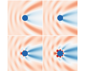
The maximum free surface elevation corresponding to the cases referenced in figures 6(a) and 7(a) is shown in figure 8 where it can be seen again how the paddles are working hard to absorb all of the available power for higher values of  $m$ where the
  $\cos m \theta$ variation in the field becomes increasingly visible.

Figure 8. For piston-like paddle motion, the maximum free surface elevation at  $ka = 2$ when springs and dampers are optimised to absorb
  $100$ % of the power available from modes: (a)
  $m=0$; (b)
  $m=1$; (c)
  $m=2$; (d)
  $m=3$; (e)
  $m=4$.
In figure 9(a) we show the proportion of power absorbed by each circular mode when paddles operating in piston-like motion are tuned to absorb 100 % of the power available in the  $m=0$ mode. Each set of results comes from different values of
  $ka$. Of course
  $100$ % of power is taken from
  $n=0$, but we again see that as
  $ka$ increases, the device is taking close to
  $100$ % available power from modes
  $n$ less than the integer part of
  $ka$. Figure 9(b) indicates the distribution of paddle amplitudes around the cylinder for these four sets of results. Optimising for total power absorption in mode
  $m=0$ implies the paddle operation is well behaved for larger values of
  $ka$ even though a significant proportion of the available power is being absorbed across a number of circular modes. For hinged paddle motion, the results are similar with roughly double the amplitudes of the piston-like motion. Figure 10 shows the maximum surface elevation corresponding to the cases referenced in figure 9.

Figure 9. For piston-like paddle motion: (a) the partition of capture factor into different circular wave modes when springs and dampers are optimised to absorb 100 % in mode  $m=0$ at different wavenumbers; (b) the corresponding distribution of paddle amplitudes around the cylinder.

Figure 10. For piston-like paddle motion, the maximum free surface elevation for springs and dampers optimised to absorb  $100$ % of the power available from the
  $m=0$ mode: (a)
  $ka = 1$; (b)
  $ka=2$; (c)
  $ka=3$; (d)
  $ka=4$.
In all the previous results, the springs and dampers have been equal around the cylinder and this means the device is omni-directional. We now consider the effect of tuning the springs and dampers to different values around the cylinder where the device operation becomes dependent on the wave heading. For simplicity, however, we only consider operation under the designed wave heading. Following the recipe for selecting the spring and damper settings in the main body of the paper, we set up the system to absorb all of available power in the first  $M+1$ circular modes and nothing from higher modes.
Figure 11 shows the maximum free surface amplitude at  $ka=2$ associated with this system for
  $M=1$ (
 $\eta = 3$) up to
  $M={4}$ (
 $\eta = {9}$). For figure 11(d) the surface elevation has exceeded the displayed vertical scale and has been top-sliced in the plot. In that case, the paddles are working hard to absorb all the available power in the first
  $M+1$ circular modes and undergoing large-amplitude excursions dominated by a
  $\cos M \theta$ variation as highlighted by figure 12. Negative springs, where they exceptionally occur, can be offset to positive springs by an increase in paddle mass and this has been confirmed numerically. The specific strategy of tuning paddles to absorb 100 % of the energy from the first
  $M+1$ modes at a specific frequency has also led to the prescription of negative dampers. In this case even though the net power is positive, some of the paddles must be driven and consume power, rather than absorb power. As can be seen in figure 12(d) this has undesirable consequences for fixed paddle parameters operating at wave frequencies for which they were not optimised including a net loss of power (illustrated by the curve for
  $M = 4$ dipping below 0).

Figure 11. For piston-like paddle motion, the maximum free surface elevation at  $ka = 2$ when springs and dampers are optimised to absorb
  $100$ % of the power available from the first
  $M+1$ modes: (a)
  $M=1$; (b)
  $M=2$; (c)
  $M=3$; (d)
  $M=4$.

Figure 12. For piston-like paddle motion at  $ka=2$ optimised to absorb
  $100$ % power from the first
  $M+1$ circular modes showing the angular variation of: (a) maximum dimensionless paddle amplitude; (b) damping parameter
  $\bar {\gamma }$; (c) spring constant
  $\bar {\kappa }$; (d) the corresponding frequency response of capture factor.
The next set set of figures in this section consider optimising the distribution of springs and dampers for  $M=3$ (
 $\eta = 7$) for
  $ka={2}$ up to
  $ka=4$. In figures 13 and 14 it is illustrated that the paddles are forced to work at amplitudes well in excess of practical limits to absorb
  $100$ % of the power from the first four circular modes from low-frequency waves (
 $ka$ small), but becomes easier for higher-frequency waves.

Figure 13. For piston-like paddle motion, the maximum free surface elevation when unequal springs and dampers are optimised to absorb  $100$ % of the power available from the first four modes (
 $M=3$,
  $\eta =7$): (a)
  $ka=2$; (b)
  $ka=3$; (c)
  $ka=4$.

Figure 14. For piston-like paddle motion optimised to absorb  $100$ % power from the first four circular modes (
 $M=3$,
  $\eta = 7$) showing the angular variation of: (a) maximum dimensionless paddle amplitude; (b) damping parameter
  $\bar {\gamma }$; (c) spring constant
  $\bar {\kappa }$; (d) the corresponding frequency response of capture factor.
The final part of the results section compares continuous paddle theory against a discrete representation of the paddles. We show a single exemplary case in figure 15 in which we fix  $\bar {\gamma } = \bar {\kappa } = 0.3$ and show the convergence of the results for
  $N$ paddles placed around the cylinder towards the results from the continuum theory. As expected, as the wavelength-to-diameter ratio reduces (
 $ka$ increases), larger values of
  $N$ are required to resolve the variations around the cylinder captured by continuum theory. However, for the range of values of
  $ka$ in which we have been interested, we can see that the continuum theory provides a good approximation to a discrete representation of
  $N \approx 24$ paddles. For example, for a
  $10$ m radius cylinder, a system of paddles of width
  $3$ m would be accurately predicted by the continuum description.

Figure 15. Capture factor against dimensionless wavenumber for different number of paddles,  $N$, with
  $\bar {\gamma }=\bar {\kappa }=0.3$: (a) piston-like paddles; (b) hinged paddles.
7. Conclusions
In this paper we have outlined a theoretical framework for extending rigid-body limits on the capacity for an axisymmetric device to absorb power from a plane incident wave. This extends established limits to wave absorption by axisymmetric devices undergoing rigid-body motion by allowing a generalised motion of the surface of the device. This general framework is developed into a WEC device by considering a circular cylinder extending throughout the fluid depth and surrounded by narrow submerged vertical paddles each attached to its own spring and damper. A continuum approximation for narrow paddles is presented and the power generated by the cylinder is determined from a system of equations which allow us to develop different strategies to determine spring and damper settings. Specifically, when all the springs and dampers are identical we can determine parameters allowing us to guarantee the absorption of  $100$ % of the energy flux available in one circular component of the plane incident wave. Allowing the springs and dampers to have different settings as a function of position around the cylinder means we can extract
  $100$ % of the available flux of energy in the first
  $M+1$ circular modes, where
  $M$ is theoretically as large as we choose. In both cases, results have shown how it is possible to achieve well in excess of the standard limit of a capture factor of
  $\eta = 3$ for rigid-body motion and capture factors in excess of
  $\eta = {8}$ have been reported in computations in this paper.
Despite these claims, there are practical considerations which will limit the value of results from this theory. Unless the cylinder is large compared to the wavelength, paddle amplitudes exceed the limits of the underpinning linearised water wave theory as the demand for power is increased leading to a compromise between power and size of device. To fully investigate this, motion constraints such as those used by Evans (Reference Evans1981) could be implemented.
The final part of the paper considers the exact description of  $N$ discrete paddles which is used to confirm that the continuum description of the paddle motion is converged to as
  $N$ increases.
Paddles are just one means by which the general theory is implemented. Other practical absorbing systems which provide the same effect such as distributing power absorption across the internal surface of a permeable axisymmetric device may work just as well (e.g. Zheng et al. Reference Zheng, Porter and Greaves2020; Garnaud & Mei Reference Garnaud and Mei2009).
Funding
S.Z. was supported by the European Union funded Marine-I (2nd phase) project (grant no. 05R18P02816). D.G. gratefully acknowledges the EPSRC for supporting part of this work through EP/S000747/1.
Declaration of interests
The authors report no conflict of interest.


 Open access