


1. Introduction
Nucleate boiling ranks among one of the most efficient heat-transfer processes. An underlying reason for this is the existence of strong temperature gradients in the close proximity of the heated surface, generated by the significant drop in temperature created between the solid wall itself and the liquid–vapour interface of the emerging bubble, which elevates the heat flux. It can be easily understood that, in the near-wall region, where the phasic interface (as perceived from the perspective of continuum fluid dynamics) comes into direct contact with the heated surface, heat fluxes of exceptional magnitude can be created. Thus, in order to precisely quantify the overall heat transfer, the near-wall morphology of growing bubbles needs to be characterised.
In the context of nucleate pool boiling, two modes of bubble growth are generally identified (Kim Reference Kim2009). The first one is the contact-line evaporation regime, in which relatively slow growth of near-spherical bubbles is observed (Fischer et al. Reference Fischer, Herbert, Slomski, Stephan and Oechsner2014; Huber et al. Reference Huber, Tanguy, Sagan and Colin2017; Bureš & Sato Reference Bureš and Sato2021c), and in which the phasic interface is terminated at the wall by a dry patch. Although this patch is sometimes assumed to be covered by an adsorbed liquid film of nanoscopic thickness (Morris Reference Morris2001; Schweikert, Sielaff & Stephan Reference Schweikert, Sielaff and Stephan2019), its presence appears not to affect the bubble-growth dynamics and, therefore, we can speak of a contact-line region, often termed the microregion (Stephan & Busse Reference Stephan and Busse1992; Janeček & Anderson Reference Janeček and Anderson2016). Here, vigorous heat- and mass-transfer processes occur; however, due to the small lateral extent of the microregion, this being O(100 nm), its importance to the overall heat-transfer mechanism is diminished (Morris Reference Morris2000; Huber et al. Reference Huber, Tanguy, Sagan and Colin2017). Nevertheless, the transfer processes within the microregion significantly alter the local liquid–vapour interface profile, giving rise to the existence of ‘apparent’ contact angles, even for perfectly wetting liquids: i.e. the angle of interfacial contact with the surface is observed to be generally non-zero for volatile liquids (Fourgeaud et al. Reference Fourgeaud, Ercolani, Duplat, Gully and Nikolayev2016; Schweikert et al. Reference Schweikert, Sielaff and Stephan2019).
The wetting conditions during bubble growth are considered to be instrumental in the appearance of the second growth regime, i.e. the microlayer evaporation regime (Afkhami et al. Reference Afkhami, Buongiorno, Guion, Popinet, Saade, Scardovelli and Zaleski2018; Guion et al. Reference Guion, Afkhami, Zaleski and Buongiorno2018; Urbano et al. Reference Urbano, Tanguy, Huber and Colin2018; Schweikert et al. Reference Schweikert, Sielaff and Stephan2019; Bureš & Sato Reference Bureš and Sato2021c). In this situation, a favourable interplay of bubble expansion and contact-line motion leads to the formation of the so-called microlayer, a thin layer of liquid adhering to the heated surface beneath the growing bubble. Owing to the minute thickness of the microlayer, very high heat fluxes can again be observed (Yabuki & Nakabeppu Reference Yabuki and Nakabeppu2014; Tanaka, Miyazaki & Yabuki Reference Tanaka, Miyazaki and Yabuki2021). In contrast to the microregion configuration, the large extent of the microlayer over the heated surface results in its evaporation being a significant contributor to the overall mass transfer of the evaporation process (Yabuki & Nakabeppu Reference Yabuki and Nakabeppu2014; Utaka et al. Reference Utaka, Hu, Chen and Morokuma2018; Tanaka et al. Reference Tanaka, Miyazaki and Yabuki2021). Indeed, in the microlayer evaporation regime, qualitatively different growth dynamics have been observed, with bubbles remaining almost hemispherical or oblate during a significant portion of the growth phase (Yabuki & Nakabeppu Reference Yabuki and Nakabeppu2014; Chen, Haginiwa & Utaka Reference Chen, Haginiwa and Utaka2017; Jung & Kim Reference Jung and Kim2018).
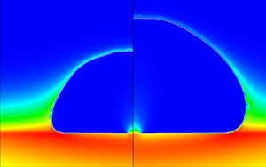
Figure 1 is a side-by-side schematic illustration of the characteristics of the two bubble-growth regimes; note that a microregion also appears in the microlayer evaporation regime, located at the inner edge of the microlayer.

Figure 1. Side-by-side illustrations of the two bubble-growth regimes: the contact-line evaporation regime (left) and the microlayer evaporation regime (right). The bottom right inset illustrates schematically the microlayer, and the left inset the microregion, where  $\theta _0$ is the physical microscopic angle and
  $\theta _{mr}$ the apparent one (see § 3.6). Note that the microregion inset is inverted with respect to the bubble in the microlayer evaporation regime. The bottom left inset illustrates the so-called ‘hump-terminated microlayer’, a shape typical of film dewetting (Snoeijer et al. Reference Snoeijer, Andreotti, Delon and Fermigier2007; Delon et al. Reference Delon, Fermigier, Snoeijer and Andreotti2008).
The importance of the microlayer, and its possible link to the critical heat flux phenomenon (Zhao, Masuoka & Tsuruta Reference Zhao, Masuoka and Tsuruta2002; Theofanous & Dinh Reference Theofanous and Dinh2006), has motivated intense scientific investigation ever since its existence was first postulated by Moore & Mesler (Reference Moore and Mesler1961) on the basis of their measurements of local temperature variations over a heated surface, and subsequently experimentally confirmed by Sharp (Reference Sharp1964) and Jawurek (Reference Jawurek1969), who employed interferometry (an imaging technique based on observation of light interference patterns) to quantify the thickness of the microlayer. Both studies employed arc lamps as light sources. The accuracy of the interferometric approach was later substantially improved with the use of lasers, recently by Gao et al. (Reference Gao, Zhang, Cheng and Quan2013), Utaka et al. (Reference Utaka, Hu, Chen and Morokuma2018), Zou, Gupta & Maroo (Reference Zou, Gupta and Maroo2018), Liu et al. (Reference Liu, Gao, Zhang and Zhang2019) and Chen et al. (Reference Chen, Haginiwa and Utaka2017, Reference Chen, Hu, Hu, Utaka and Mori2020), to provide a detailed description of the evolution of the microlayer structure. Further methods of microlayer investigation include the laser extinction method, which can measure the thickness locally to very high precision, based on the attenuation of a laser beam when it passes through a liquid film (Utaka, Kashiwabara & Ozaki Reference Utaka, Kashiwabara and Ozaki2013; Utaka et al. Reference Utaka, Kashiwabara, Ozaki and Chen2014).
Additionally, the heat-transfer characteristics of the microlayer have been measured both locally, using microsensors (Yabuki & Nakabeppu Reference Yabuki and Nakabeppu2014, Reference Yabuki and Nakabeppu2016; Yabuki et al. Reference Yabuki, Samaroo, Nakabeppu and Kawaji2015; Yabuki & Nakabeppu Reference Yabuki and Nakabeppu2017), and globally, using infrared (IR) cameras (Duan et al. Reference Duan, Phillips, McKrell and Buongiorno2013; Surtaev, Serdyukov & Chernyavskiy Reference Surtaev, Serdyukov and Chernyavskiy2017; Serdyukov et al. Reference Serdyukov, Surtaev, Pavlenko and Chernyavskiy2018; Kangude & Srivastava Reference Kangude and Srivastava2020; Tanaka et al. Reference Tanaka, Miyazaki and Yabuki2021). Such experiments have provided information on heat-flux conditions within the microlayer, and its significance in the overall boiling process. Finally, Jung & Kim (Reference Jung and Kim2014, Reference Jung and Kim2018, Reference Jung and Kim2019) and Giustini, Kim & Kim (Reference Giustini, Kim and Kim2020b) combined measurements of surface heat-transfer characteristics using IR thermometry with microlayer profile evaluation using laser interferometry, producing a comprehensive set of experimental data on nucleate boiling in the microlayer regime.
Although modern, high-resolution experimental techniques can provide detailed information on the actual microlayer dynamics, several limitations and deficiencies in the approach can be identified. Measurements of microlayer thickness are often indirect and/or rely either on assumptions, such as zero flow in the microlayer (Utaka et al. Reference Utaka, Kashiwabara and Ozaki2013; Yabuki & Nakabeppu Reference Yabuki and Nakabeppu2014), or on indirect numerical techniques (Bucci et al. Reference Bucci, Richenderfer, Su, McKrell and Buongiorno2016), the uncertainties of which need to be carefully evaluated (Kim et al. Reference Kim, Sergis, Kim and Hardalupas2020). Furthermore, an experimental set-up can accommodate only a limited number of diagnostic systems, reducing the amount of information that can be obtained in a synchronous way. The possibility of generalisation of the experimental results is also hindered by the limited combinations of test fluids that can be employed, the working conditions and the inability to independently vary the controlling parameters, such as the material properties, in a straightforward manner.
One possibility to alleviate these restrictions is offered by the use of direct numerical simulation (DNS) for modelling the bubble-growth process through the direct numerical solution of the governing equations of continuum fluid dynamics. The microlayer can then be explicitly resolved within the computations, and comprehensive information extracted. A validated DNS code can also be used in combination with an experiment, to complement the measured data, or on its own, to perform parametric studies outside the scope of the standard working fluids, and to study system sensitivity to the input parameters and applied boundary conditions (BCs).
In recent years, pioneering DNS studies on boiling with a resolved microlayer (DNS-BRM) have been conducted, thanks to the advent of high-performance computing, coupled with the continuous development of advanced numerical methods for multiphase computational fluid dynamics (MCFD). Note that all the numerical works referenced below have employed an axisymmetric cylindrical representation of the problem, since a full, three-dimensional (3-D) solution lies beyond the limits imposed by present-day computational resources, and the extremely high resolution demanded to perform a DNS-BRM study. Hänsch & Walker (Reference Hänsch and Walker2016) succeeded in simulating hydrodynamic microlayer formation with the time-dependent bubble-growth rate deduced from the analytical solution of Scriven (Reference Scriven1959). Similar work has been performed by Guion et al. (Reference Guion, Afkhami, Zaleski and Buongiorno2018) under the tenet that bubble growth takes place principally within the inertial regime (Faghri & Zhang Reference Faghri and Zhang2006), with the constant expansion rate given by the simplified formula of Mikic, Rohsenow & Griffith (Reference Mikic, Rohsenow and Griffith1970) for near-wall expansion. Heat transfer was first included in a DNS-BRM approach by Urbano et al. (Reference Urbano, Tanguy, Huber and Colin2018). A rigorous computational exercise was performed, utilising a computational mesh with submicrometre resolution, and a criterion proposed to distinguish between the contact-line and microlayer evaporation regimes, based on the results. However, the conjugate heat-transfer problem between the solid and the fluids (liquid and vapour) was not solved explicitly: rather, the wall was assumed to be uniformly superheated and isothermal. Furthermore, interfacial heat-transfer resistance (IHTR), a phenomenon also currently under investigation in the context of nucleate boiling (Giustini et al. Reference Giustini, Jung, Kim and Walker2016), was not considered.
In their more recent work, Hänsch & Walker (Reference Hänsch and Walker2019) coupled their hydrodynamic solver with a prescribed Scriven-type growth rate to their own microlayer depletion model, represented by the solution of the steady-state one-dimensional (1-D) heat conduction equation, while the wall temperature distribution was obtained by solving the unsteady conduction problem within the solid substrate. The depletion model itself took into account IHTR, with a value of the resistance based on the experiments of Jung & Kim (Reference Jung and Kim2014). Only limited comparison of the microlayer evolution with experimental data was performed, with the growth rate of the simulated bubble prescribed a priori to match the experimental measurements. A purely hydrodynamic DNS-BRM investigation with a Scriven-type fixed growth-rate model was also undertaken by Giustini et al. (Reference Giustini, Kim, Issa and Bluck2020a); similar comparisons with the experiments of Jung & Kim (Reference Jung and Kim2018) as by Hänsch & Walker (Reference Hänsch and Walker2019) were made. Using a Mikic-type fixed growth rate, Giustini et al. (Reference Giustini, Kim, Issa and Bluck2020a) also simulated microlayer formation during the boiling of liquid sodium, whose material properties differ significantly from those of the typically studied fluids, i.e. water and ethanol under atmospheric conditions.
In spite of the undeniable progress being made in the field of DNS-BRM in recent years, a survey of the above-referenced works reveals that several issues still need to be resolved:
(i) No actual validation of the numerical approaches employed has so far been performed, thereby reducing the confidence level of the predictions.
(ii) Heat transfer has been included only in the fluid domain (Urbano et al. Reference Urbano, Tanguy, Huber and Colin2018), through reduced-order modelling (Hänsch & Walker Reference Hänsch and Walker2019), or in many cases not at all (Hänsch & Walker Reference Hänsch and Walker2016; Guion et al. Reference Guion, Afkhami, Zaleski and Buongiorno2018; Giustini et al. Reference Giustini, Kim, Issa and Bluck2020a). The role of IHTR in the heat-transfer mechanism in particular is still an open issue.
(iii) The role of wetting conditions in microlayer dynamics has also not been addressed adequately: i.e. only static contact angles have been considered so far, an exception being the work of Giustini et al. (Reference Giustini, Kim, Issa and Bluck2020a), who preferred to employ a vanishing contact angle BC. Urbano et al. (Reference Urbano, Tanguy, Huber and Colin2018) attributed dewetting to be the principal driving mechanism for microlayer destruction. In our recent work (Bureš & Sato Reference Bureš and Sato2021c), we have highlighted the role of numerical slip (Afkhami et al. Reference Afkhami, Buongiorno, Guion, Popinet, Saade, Scardovelli and Zaleski2018) in simulations of microlayer dynamics, and proposed that this could artificially promote dewetting in DNS-BRM, and stressed the need for the careful implementation in the code of the actual wetting phenomenon. Furthermore, the value of the contact angle to be imposed in the simulation is often unclear, since dynamic wetting conditions of volatile liquids can significantly differ from static, adiabatic conditions (Raj et al. Reference Raj, Kunkelmann, Stephan, Plawsky and Kim2012; Janeček & Nikolayev Reference Janeček and Nikolayev2013; Fourgeaud et al. Reference Fourgeaud, Ercolani, Duplat, Gully and Nikolayev2016; Schweikert et al. Reference Schweikert, Sielaff and Stephan2019).
For these reasons, we have decided to validate a computational method for DNS-BRM studies with a focus on the microscopic physics of the problem; to this end, we have adapted the open-source code PSI-BOIL for such application. (The code is available at https://github.com/PSI-NES-LSM-CFD/PSI-Boil.) We have introduced the axisymmetric cylindrical geometric volume-of-fluid (GVOF) method for interface tracking (Bureš, Sato & Pautz Reference Bureš, Sato and Pautz2021), and coupled it with the existing sharp-interface heat- and mass-transfer model within PSI-BOIL, and with the phasic velocity extrapolation algorithm of Malan et al. (Reference Malan, Malan, Zaleski and Rousseau2021), but with several modifications (Bureš & Sato Reference Bureš and Sato2021b). As reference data for validation, we have acquired comprehensive measurements of first-bubble growth in a microlayer evaporation regime taken at the Massachusetts Institute of Technology by Bucci (Reference Bucci2020), partially presented in Bucci, Buongiorno & Bucci (Reference Bucci, Buongiorno and Bucci2021). In the present study, we have used the data for which the experimentalists had the highest confidence in the fidelity of the reported results, corresponding to a situation with an applied heat flux of  $425~{\rm kW}~{\rm m}^{-2}$.
The present paper is a continuation of our previous work (Bureš & Sato Reference Bureš and Sato2021c), in which we were concerned with deriving a theoretical description of the conditions leading to microlayer formation. Here, we focus on the development and validation of a computational method for DNS-BRM studies, and the application of this method to the analysis of the distribution of the microlayer thickness following its initial formation. In § 2, we present specific details of the method, while in § 3 the topic of IHTR is discussed, with the values of the resistance for use in the simulations determined from appropriate experimental data. Expressions adopted for the dynamic contact angle, in lieu of a definitive experimental value, are also discussed. The validation of the overall method against the measurements of Bucci (Reference Bucci2020) is given in § 4; good agreement with the experimental data is demonstrated, and points of concern highlighted. In § 5, we review sensitivities to particular simulation settings and assumptions. In § 6, we perform a sensitivity study of the microlayer thickness following its formation, recovering a semi-empirical relation describing its distribution. Finally, overall conclusions are drawn in § 7. Furthermore, in Appendix B, a first demonstration of DNS of boiling with an explicitly resolved microlayer in 3-D Cartesian coordinates is also presented.
(The reader should note that, in this paper, the work of Professor M. Bucci (Bucci et al. Reference Bucci, Richenderfer, Su, McKrell and Buongiorno2016) and the work of Mr M. Bucci (Bucci Reference Bucci2020), as well as their joint publication (Bucci et al. Reference Bucci, Buongiorno and Bucci2021), are referenced. We bring this to the reader's attention to avoid possible confusion of these two researchers.)
2. Governing equations
PSI-BOIL is an open-source MCFD code developed at the Paul Scherrer Institute in Switzerland. The primary mission of its eleven-year-long development is to promote basic computational research of volatile multiphase flows in the framework of continuum theory. To this end, the governing equations for incompressible flows with phase change are solved, including phase, momentum, mass and energy exchanges. The solution algorithm is described in detail by Bureš et al. (Reference Bureš, Sato and Pautz2021) and Bureš & Sato (Reference Bureš and Sato2021b). Below, a brief summary is given, special attention being paid to the numerical treatment of the solid substrate in nucleate boiling, a topic not covered in our previous papers. In the present context, all the governing equations are solved in a two-dimensional (2-D), axisymmetric cylindrical geometry, though a full 3-D option is available in the code. The verification and validation for two-phase flows with and without phase change are reported in Bureš et al. (Reference Bureš, Sato and Pautz2021) and Bureš & Sato (Reference Bureš and Sato2021b), and they are not repeated in this paper.
2.1. Phase conservation and interface tracking
Two phases, liquid and vapour, are included in PSI-BOIL. Their mass densities are considered to be constant,  $\rho _l$ and
  $\rho _v$ (
 ${\rm kg}~{\rm m}^{-3}$); thus, to track the phasic distribution, it is sufficient to solve the transport equation for the liquid volume fraction,
  $\phi$, defined for a computational cell with volume
  $\Delta V$ (m
 $^3$) as
 \begin{equation} \phi = \frac{V_l}{\Delta V}, \end{equation}
where  $V_l$ is the volume of the cell occupied by liquid. The vapour volume fraction is then
  $(1-\phi )$.
The transport equation for  $\phi$ can be derived from general two-phase integral balance considerations and reads (Bureš & Sato Reference Bureš and Sato2021b)
 \begin{equation} \frac{\partial\phi}{\partial t} ={-}\boldsymbol{\nabla} \boldsymbol{\cdot} (\phi \boldsymbol{u}_l) - \frac{{\dot{m}}'''}{\rho_l} ={-} \frac{1}{\Delta V} \sum_i F_{l,i} - \frac{{\dot{m}}'''}{\rho_l}. \end{equation}
Here,  $\boldsymbol {u}_l$ (
 ${\rm m}~{\rm s}^{-1}$) is the (divergence-free) liquid velocity field, satisfying the incompressibility condition, and computed from a modified version of the extrapolation algorithm of Malan et al. (Reference Malan, Malan, Zaleski and Rousseau2021), without which consistent advection of
  $\phi$ in the presence of phase change would not be possible. Furthermore,
  $\dot {m}'''$ is the evaporative mass source density
  $({\rm kg}~({\rm m}^{3}~{\rm s})^{-1})$. The advection term is treated using the GVOF method of Weymouth & Yue (Reference Weymouth and Yue2010), expressed in terms of the liquid surface flows
  $F_{l,i}$
  $({\rm m}^3~{\rm s}^{-1})$ defined for each bounding surface
  $i$ of the computational cell. Equation (2.2) is discretised in explicit form as follows:
 \begin{gather} \frac{\phi^\star{-}\phi^{n}}{\Delta t} ={-} \frac{\dot{m}'''}{\rho_l}, \end{gather}
 \begin{gather}\frac{\phi^{n+1}-\phi^\star}{\Delta t} ={-} \frac{1}{\Delta V}\sum_i F_{l,i}, \end{gather}
where  $\Delta t$ (s) is the discrete time step,
  $\phi ^\star$ is an intermediate value of the volume fraction, while
  $n$ and
  $n+1$ indicate the previous and new time steps, respectively. The evaporative mass source density needed for the phase-change step (2.3) is calculated according to
 \begin{equation} \dot{m}''' = a_\gamma \frac{1}{L} (\lambda_l\boldsymbol{\nabla} T|_{\gamma,l} \boldsymbol{\cdot}\boldsymbol{n}-\lambda_v\boldsymbol{\nabla} T|_{\gamma,v} \boldsymbol{\cdot}\boldsymbol{n}). \end{equation}
Here,  $a_\gamma$ (m
 $^2$ m
 $^{-3}$) is the interfacial area density, computed by means of the marching cubes algorithm (Lorensen & Cline Reference Lorensen and Cline1987), and based on the local
  $\phi$ stencil, adapted for use in axisymmetric geometry;
  $L$ (J kg
 $^{-1}$) is the latent heat of vaporisation; and
  $\lambda _l$ and
  $\lambda _v$ are the liquid and vapour thermal conductivities
  $({\rm W}~({\rm m}~{\rm K})^{-1})$, respectively. Furthermore,
  $\boldsymbol {\nabla } T|_{\gamma,l}$ and
  $\boldsymbol {\nabla } T|_{\gamma,v}$ are the temperature gradients on the liquid and vapour sides of the interface
  $({\rm K}~{\rm m}^{-1})$. They are calculated using fourth-order-accurate upwind differences for non-uniform grids, evaluated at the interface; details appear in Bureš & Sato (Reference Bureš and Sato2021b). The unit normal vector to the interface pointing from the vapour phase to the liquid phase,
  $\boldsymbol {n}$, is evaluated using the ELVIRA algorithm of Pilliod & Puckett (Reference Pilliod and Puckett2004). Note that the interfacial jump in kinetic energy is neglected, being in general small in comparison to the latent heat of phase transition, as can be deduced from a scaling analysis.
The second step in the solution of the transport equation (2.4) is performed using the directional-split, bounded-conservative GVOF algorithm of Weymouth & Yue (Reference Weymouth and Yue2010), also adapted for use in axisymmetric geometry.
2.2. Momentum conservation
The two-phase momentum conservation equations, written in the single-fluid approximation, read as follows:
 \begin{equation} \rho \frac{\text{D}\boldsymbol{u}}{\text{D}t} ={-}\boldsymbol{\nabla} p + \boldsymbol{\nabla}\boldsymbol{\cdot} [\mu(\boldsymbol{\nabla} \boldsymbol{u}+(\boldsymbol{\nabla}\boldsymbol{u})^{\rm T})] + \rho \boldsymbol{g} + \,\boldsymbol{f}_\sigma. \end{equation}
Note that the recoil pressure due to phase change has not been considered, since it is generally negligible within the present application area, as we concluded using a scaling analysis. In this equation,  $\boldsymbol {u}$ is the single-fluid mechanical velocity,
  $p$ is the pressure (Pa),
  $\boldsymbol {g}$ is the gravitational acceleration (
 ${\rm m}~{\rm s}^{-2}$),
  $\,\boldsymbol {f}_\sigma$ is the surface-tension force density
  $({\rm N}~{\rm m}^{-3})$ and
  $\rho$ is the mixture density, given by
 \begin{equation} \rho = \phi\rho_l + (1-\phi)\rho_v. \end{equation}
In the single-fluid approximation,  $\boldsymbol {u}$ is taken to be continuous across the interface and the stress balance at the interface is not represented exactly. Instead, a heuristic harmonic mixing law is applied for the computation of mixture dynamic viscosity
  $\mu$
$\mu$  $({\rm Pa}~{\rm s})$ in the vicinity of the interface. In the simulations shown below, we use the harmonic mixing law (Prosperetti Reference Prosperetti2002):
 \begin{equation} \frac{1}{\mu} = \frac{\phi}{\mu_l} + \frac{1-\phi}{\mu_v}. \end{equation}
 We have also conducted simulations of the validation problem presented in § 4 using other heuristic viscosity averaging schemes; no discernible differences in the overall dynamics have been observed. Note that, since the near-interface stress balance is anyway treated only approximately, we neglect the  $(\boldsymbol {\nabla }\boldsymbol {u})^{\rm T}$ term in (2.6) for reasons of simplicity and robustness of the numerical implementation.
In PSI-BOIL, (2.6) is solved in the finite-volume formulation:
 \begin{align} &\rho\left(\frac{\partial\boldsymbol{u}}{\partial t}\,\Delta V + \sum_i (\boldsymbol{u}\otimes\boldsymbol{u}) \boldsymbol{\cdot}\Delta\boldsymbol{S}_i - (\boldsymbol{\nabla}\boldsymbol{\cdot} \boldsymbol{u})\boldsymbol{u}\,\Delta V \right) \nonumber\\ & \quad ={-} \boldsymbol{\nabla} p\, \Delta V + \sum_i \mu\boldsymbol{\nabla}\boldsymbol{u}\boldsymbol{\cdot} \Delta\boldsymbol{S}_i + \rho\boldsymbol{g}\,\Delta V + \,\boldsymbol{f}_\sigma \,\Delta V. \end{align}
The discretised variables are arranged using the staggered-grid approach of Harlow & Welch (Reference Harlow and Welch1965). For the spatial discretisation, a second-order-accurate, central-difference scheme and a second-order flux-limiting, total-variation-diminishing (TVD) scheme (Roe Reference Roe1986) are used for the diffusion and advection terms, respectively. For the time discretisation, backward and forward Euler methods are used to treat the diffusion and advection terms, respectively. The Boussinesq approximation (Gray & Giorgini Reference Gray and Giorgini1976) for density is adopted: i.e. the variability of densities with temperature is only taken into account in the calculation of the buoyancy force. The surface-tension force density is given by
 \begin{equation} \boldsymbol{f}_\sigma = \sigma \kappa a_\gamma \boldsymbol{n}, \end{equation}
with  $\sigma$
  $({\rm N}~{\rm m}^{-1})$ being the surface tension (assumed constant), and
  $\kappa$
  $({\rm m}^{-1})$ the interfacial curvature, which is taken to be positive if the centre of curvature is in the liquid phase and negative otherwise. Note that Marangoni stresses (Faghri & Zhang Reference Faghri and Zhang2006) have been neglected based on our analysis of the heat-flux conditions within the microlayer for the experiment discussed in § 4 (see § 3 for the description of the relation between heat flux and interfacial temperature). Additionally, disjoining pressure (Faghri & Zhang Reference Faghri and Zhang2006; Janeček & Nikolayev Reference Janeček and Nikolayev2013) has not been considered, since this phenomenon becomes relevant at length scales well below the grid resolution employed in the simulations described in this paper.
As is common practice, (2.10) is discretised using the continuum surface force approach of Brackbill, Kothe & Zemach (Reference Brackbill, Kothe and Zemach1992):
 \begin{equation} \boldsymbol{f}_\sigma = \sigma\kappa \frac{2\rho}{\rho_l+\rho_v}\, \frac{\boldsymbol{\nabla}\rho}{\rho_l-\rho_v}. \end{equation}
In our approach, the curvature  $\kappa$ is calculated by means of the height function method (Popinet Reference Popinet2018), with a
  $3 \times 7$ stencil utilising the local-topology adaptation approach of López et al. (Reference López, Zanzi, Gómez, Zamora, Faura and Hernández2009), again modified for use in axisymmetric geometry.
2.3. Mass conservation
As the densities of the phases are here considered constant, the mass continuity equation may be conveniently replaced by the equivalent volume-conservation condition, resulting from the application of the two-phase divergence theorem, as
 \begin{equation} \sum_i \boldsymbol{u}\boldsymbol{\cdot}\Delta \boldsymbol{S}_i = \dot{m}'''\left(\frac{1}{\rho_v}-\frac{1}{\rho_l}\right)\Delta V. \end{equation}
Here,  $\Delta \boldsymbol {S}_i$ is the (outward-oriented) area of the bounding surface
  $i$ within the given computational cell. This condition is enforced at each time step by the projection algorithm of Chorin (Reference Chorin1968), which consists of solving the discrete Poisson equation for the pressure
  $p$ at the advanced time step
  $n+1$,
 \begin{equation} \sum_i \frac{\Delta t}{\rho}\,\boldsymbol{\nabla} p^{n+1} \boldsymbol{\cdot} \Delta\boldsymbol{S}_i = \sum_i \boldsymbol{u}^\star \boldsymbol{\cdot} \Delta\boldsymbol{S}_i - \dot{m}^{\prime\prime\prime,n}\left(\frac{1}{\rho_v}-\frac{1}{\rho_l}\right) \Delta V, \end{equation}
followed by the projection step,
 \begin{equation} \boldsymbol{u}^{n+1} = \boldsymbol{u}^\star{-} \frac{\Delta t}{\rho} \, \boldsymbol{\nabla} p^{n+1}. \end{equation}
In these equations,  $\boldsymbol {u}^\star$ is a tentative estimate of the velocity field, obtained from the numerical solution of the following equation:
 \begin{align} &\frac{\rho^n\boldsymbol{u}^\star}{\Delta t}\,\Delta V - \sum_i \mu\boldsymbol{\nabla}\boldsymbol{u}^{{\star}}\boldsymbol{\cdot} \Delta\boldsymbol{S}_i \nonumber\\ & \quad = \rho^n\left(\frac{\boldsymbol{u}^n}{\Delta t}\,\Delta V -\sum_i (\boldsymbol{u}^n\otimes\boldsymbol{u}^n) \boldsymbol{\cdot} \Delta\boldsymbol{S}_i + (\boldsymbol{\nabla}\boldsymbol{\cdot}\boldsymbol{u}^n) \boldsymbol{u}^n\, \Delta V \right) + \rho^n\boldsymbol{g}\,\Delta V + \,\boldsymbol{f}^n_\sigma\,\Delta V. \end{align}
Note that, by assuming the validity of (2.12), we are effectively identifying the single-fluid velocity  $\boldsymbol {u}$ with the volume-averaged velocity.
2.4. Energy conservation
The energy conservation equation is the only balance equation in PSI-BOIL not recast in integral form, but rather solved in a finite-difference approximation to its differential form:
 \begin{gather} C_{p,l} \left(\frac{\partial T}{\partial t} + \boldsymbol{\nabla}\boldsymbol{\cdot}(T\boldsymbol{u}_l) -T(\boldsymbol{\nabla}\boldsymbol{\cdot}\boldsymbol{u}_l)\right)= \lambda_l\nabla^2 T \quad \text{in the liquid}, \end{gather}
 \begin{gather}C_{p,v} \left(\frac{\partial T}{\partial t} + \boldsymbol{\nabla}\boldsymbol{\cdot}(T\boldsymbol{u}_v) -T(\boldsymbol{\nabla}\boldsymbol{\cdot}\boldsymbol{u}_v)\right)= \lambda_v\nabla^2 T\quad \text{in the vapour}, \end{gather}
 \begin{gather}T = T_\gamma\quad \text{at the interface}. \end{gather}
The equation is discretised separately in the liquid and vapour regions of the domain, with the phasic interface being treated as an internal boundary, unlike for the momentum equations. Since the finite-volume scheme cannot be easily employed in the vicinity of the phasic interface, where the computational cells are cut, the finite-difference approach is employed here. In the above equations,  $C_{p,l}=\rho _l c_{p,l}$ and
  $C_{p,v}=\rho _v c_{p,v}$ are the volumetric heat capacities
  $({\rm J}~({\rm m}^3~{\rm K})^{-1})$ for the liquid and vapour, respectively; and
  $c_{p,l}$ and
  $c_{p,v}$ are the respective specific heat capacities
  $({\rm J}~({\rm kg}~{\rm K})^{-1})$.
Note that the form of the energy conservation equation presented here could be derived from the internal energy balance equation, assuming zero internal heating and neglecting heat generation due to viscous stress work and compressibility effects, all justified within the context of the present application. A sharp-interface, finite-difference algorithm is employed for its spatial discretisation: the diffusion term is treated implicitly, with the interfacial position resolved with subgrid accuracy, utilising the information provided by the GVOF interface-tracking method referred to earlier. A three-point, central-difference scheme is employed, of second-order accuracy for steady-state conditions. For problems depending on the gradients of the solution, such as the bubble-growth problem of Scriven (Reference Scriven1959), first-order accuracy is retrieved (Gibou et al. Reference Gibou, Fedkiw, Cheng and Kang2002). (We thank one of the referees for clarifying this point during the review process.) The advection terms are treated explicitly, employing a second-order TVD scheme. The phasic velocities,  $\boldsymbol {u}_l$ and
  $\boldsymbol {u}_v$, are obtained from a variation of the extrapolation algorithm of Malan et al. (Reference Malan, Malan, Zaleski and Rousseau2021) and ‘ghost’ values of temperature are calculated by means of linear extrapolation across the interface, assuming continuity of temperature at the interface itself, calculated at the appropriate interface position. Note that the temperature gradient is not continuous at the interface, due to the step change in the thermal conductivities occurring there, and the presence of a non-zero phase-change rate (2.5).
The interfacial temperature  $T_\gamma$ is assumed to be constant and equal to the saturation temperature at the prevailing system pressure: see § 3 for a discussion of the role and implementation of the IHTR.
2.5. Treatment of the solid
In the solid part of the domain, only heat conduction needs to be considered:
 \begin{equation} C_{p,s}\frac{\partial T}{\partial t} = \sum_i\lambda_s\boldsymbol{\nabla} T|_i \boldsymbol{\cdot}\frac{\Delta\boldsymbol{S}_i}{\Delta V} + q, \end{equation}
where  $q$
$q$  $({\rm W}~{\rm m}^{-3}$) is the volumetric heat source, e.g. due to electrical resistance heating. Note that a finite-volume formulation, rather than a finite-difference one, is employed, since it was found to have better convergence characteristics in the presence of a heat source in preliminary 1-D test studies. With the solid assumed to be a single phase, the finite-volume formulation can be employed without issues. If it is composed of several layered materials, simple averaging based on volume fractions is used to obtain the cell-specific values of
  $C_{p,s}$ and
  $\lambda _s$. This treatment is exact for
  $C_{p,s}$ but only approximate for
  $\lambda _s$, the degree of approximation depending on the grid resolution.
2.5.1. Wall boundary conditions for heat transfer
At the solid–fluid boundary, continuity of heat flux is assumed. The existence of a temperature contact discontinuity is permitted, and modelled in terms of a contact heat-transfer resistance  $\mathcal {R}_c$
  $({\rm K~m}^2~{\rm W}^{-1})$. As a result, the solid-side and fluid-side boundary temperatures can be derived from
 \begin{gather} T_{{b},s} = \frac{(\mathcal{R}_c+\mathcal{R}_f) T_s+ \mathcal{R}_s T_f}{\mathcal{R}_c+\mathcal{R}_f+\mathcal{R}_s } = \frac{(\mathcal{R}_c+\Delta z_f/\lambda_f) T_s+ (\Delta z_s/\lambda_s) T_f}{\mathcal{R}_c+\Delta z_f/\lambda_f +\Delta z_s/\lambda_s }, \end{gather}
 \begin{gather}T_{{b},f} = \frac{\mathcal{R}_f T_s+ (\mathcal{R}_c+\mathcal{R}_s) T_f}{\mathcal{R}_c+\mathcal{R}_f+\mathcal{R}_s } = \frac{(\Delta z_f/\lambda_f) T_s+ (\mathcal{R}_c+\Delta z_s/\lambda_s) T_f}{\mathcal{R}_c+\Delta z_f/\lambda_f +\Delta z_s/\lambda_s}, \end{gather}
where  $T_s$ is the temperature in the solid at distance
  $\Delta z_s$ from the boundary, and
  $T_f$ is the temperature in the fluid at distance
  $\Delta z_f$ from the boundary; this could be either the distance to the nearest mesh point or that to the phasic interface.
For the purpose of implicit discretisation of the Laplacian operator in (2.16) and (2.17), we start with a generic, three-point central-difference formula:
 \begin{equation} \frac{\partial^2 T}{\partial z^2}\approx K_P (T_P-T_C) + K_B (T_b-T_C). \end{equation}
Here,  $T_C$ is the temperature at the point where the difference is calculated; for illustration, we choose the solid-adjacent fluid cell, shown as the central cell in figure 2. The coefficients
  $K_P$ and
  $K_B$ are functions of the distances to the solid–fluid boundary
  $\Delta z_p$ and
  $\Delta z_b$, also illustrated in figure 2. Assuming that
  $T_b$ has been computed from
  $T_M$ and
  $T_C$ using (2.21), we can then develop the second term on the right-hand side of (2.22) as follows:
 \begin{align} K_B (T_b - T_C) &= K_B\left(\frac{\mathcal{R}_M T_C + \mathcal{R}_C T_M}{\mathcal{R}_M+\mathcal{R}_C}-T_C\right) = K_B\left(\frac{\mathcal{R}_C T_M-\mathcal{R}_C T_C}{\mathcal{R}_B+\mathcal{R}_C}\right)\nonumber\\ &= K_B\frac{\mathcal{R}_C}{\mathcal{R}_M+\mathcal{R}_C} (T_M - T_C)\equiv K_M (T_M - T_C). \end{align}
Figure 2. Schematic representation of the stencil used for the implicit discretisation of the heat diffusion term of the energy transport equation in the vicinity of a solid–fluid boundary, indicated here by the thick vertical line:  $T_{b,s}$ and
  $T_{b,f}$ are the solid-side and liquid-side boundary temperatures, respectively.
Similar estimations are used within the solid finite-volume formulation on the solid side of the boundary. Thus, the conjugate heat-transfer problem between the solid and the fluid can be solved by means of a fully coupled algorithm, with heat conduction treated implicitly on both the fluid and solid sides of the boundary. Note that, in our application domain, the physical solid–liquid contact resistance is assumed to be zero; we use  $\mathcal {R}_c$, however, for reduced-order modelling of IHTR. This is discussed further in § 3.5.
2.5.2. Wall boundary conditions for interface reconstruction
Our subgrid-accurate implementation of phase change using (2.5) necessitates the calculation of the interfacial area density  $a_\gamma$ in all wall-adjacent cells. The nodal values of
  $\phi$ required by the marching cubes algorithm (Lorensen & Cline Reference Lorensen and Cline1987) necessitate the use of ghost values in the wall cells. These are obtained using the following iterative extrapolation procedure:
(i) Perform the GVOF reconstruction of the interfacial geometry in wall-adjacent cells, utilising only information in the fluid cells themselves. Here, GVOF reconstruction means computing normal vectors and line constants defining the GVOF interfacial orientation based on the
 $\phi$ stencil described in Bureš et al. (Reference Bureš, Sato and Pautz2021).
(ii) Extend the linear interface from wall-adjacent cells to the ghost cells to obtain
$\phi ^{{ghost}}$.(iii) Perform the GVOF reconstruction of the interfacial geometry in wall-adjacent cells again, utilising the full stencil this time, and including the ghost-cell estimates. Note that the normal vector calculated at this step could be different from the one obtained in step (i).
(iv) Compare the new normal vector field with the previous estimate. If the change is outside the specified tolerance, go back to step (ii) and repeat.


In practical terms, the method converges very rapidly, requiring only one or two iterations to reach negligible variation of the normal vector field, as stipulated in the predefined tolerances. A schematic representation of the result of the wall iterative extrapolation procedure is presented in figure 3.

Figure 3. Schematic representation of the wall iterative extrapolation procedure. Note that the shape of the interface in the fluid domain is slightly perturbed in the process due to realignment of the normal vector. Note also that the linear extension of the interface is limited only to the adjacent ‘ghost’ cell.
2.5.3. Wall boundary conditions for curvature
Multiphase DNS requires the implementation of hydrodynamic BCs at the solid wall; in this work, we assume the natural no-slip/no-penetration BC for velocity. Consequently, the hydrodynamic BC reduces to a contact-angle condition (i.e. a Dirichlet BC for the interfacial slope at the wall), which augments the computation of the surface tension force (2.11) in the near-wall cells. In this work, we explicitly impose the contact angle using the height-function approach of Afkhami & Bussmann (Reference Afkhami and Bussmann2008), again adapted for axisymmetric geometry. The contact angle model employed in our simulations is explained fully in § 3.6.
2.6. Overall solution algorithm
In summary, the following algorithm is employed to solve the governing equations in PSI-BOIL:
(i) Calculate the interfacial area density
$a_\gamma$ using the marching cubes algorithm needed for (2.5).(ii) Calculate the mass transfer
$\dot {m}'''$ between the phases directly using (2.5).(iii) Calculate the curvature
$\kappa$ using the height-function method, and use it to estimate the surface tension force $\,\boldsymbol {f}_\sigma$ via (2.11).(iv) Solve the momentum conservation equations (2.9) to obtain a tentative estimate of the velocity field
$\boldsymbol {u}^\star$.(v) Solve the Poisson equation for pressure, (2.13), and project the tentative velocity field
$\boldsymbol {u}^\star$ to ensure volume conservation using (2.14), obtaining a new estimate of the velocity field $\boldsymbol {u}$.(vi) Calculate the intermediate volume fraction field using (2.3).
(vii) Calculate the liquid and vapour velocity fields
$\boldsymbol {u}_l$ and $\boldsymbol {u}_v$ (individual phasic velocities) using our version of the extrapolation algorithm of Malan et al. (Reference Malan, Malan, Zaleski and Rousseau2021), as detailed in Bureš & Sato (Reference Bureš and Sato2021b).(viii) Advect the intermediate volume fraction field using directional splitting, (2.4).
(ix) Ensure energy conservation by the simultaneous solution of (2.16), (2.17) and (2.19).
(x) Advance the time step.
(xi) Go back to step (i).


3. Interfacial heat-transfer resistance
In § 2.4, we indicated that the liquid and vapour phases are constrained during the solution of the energy conservation equation by a Dirichlet BC for temperature at the phasic interfaces. An estimate of the interfacial temperature  $T_\gamma$ can then be derived from the assumption of thermostatic equilibrium: i.e. that the temperature is continuous across the interface, with
  $T_\gamma$ equal to the saturation temperature at the ambient system pressure
  $T_{{sat}}$, with local pressure variations and the Kelvin effect (Thomson Reference Thomson1872) being neglected.
3.1. Discrepancy
Although the above assumption is generally acceptable for single-component multiphase systems (Ishii & Hibiki Reference Ishii and Hibiki2011), it is known that it can induce non-negligible error in the calculation of heat flow through the microregion and microlayer of an expanding bubble from a heated surface (Giustini et al. Reference Giustini, Jung, Kim and Walker2016). For illustration, consider a typical data point from the experiment of Bucci (Reference Bucci2020), with a measured wall superheat  $\Delta T_{{wall}} \!=\! T_{{wall}} - T_{{sat}}$ in the range of 5–10 K. Though the microlayer thickness
  $d$ (m) was not explicitly measured in this experiment, during evaporation, values of
  $d = O(100~\text {nm})$ would be expected, as indicated by other recent experiments (e.g. Chen et al. Reference Chen, Hu, Hu, Utaka and Mori2020). Assuming steady-state 1-D conduction through the liquid microlayer beneath the expanding bubble (see § 4 for a discussion of the validity of this assumption), this gives for the heat flux
  $j_q$ (W m
 $^{-2}$):
 \begin{equation} j_q = \lambda_l\frac{\Delta T_{{wall}}}{d} = O(10~\text{MW}~\text{m}^{{-}2}). \end{equation}
Such values should thus be routinely observed during an experiment of this type, but the maximal values reported by Bucci (Reference Bucci2020) are in the region of 2 MW m $^{-2}$ in the 5–10 K superheat range. Such a discrepancy is not exceptional, and has often been reported in the literature (e.g. Giustini et al. Reference Giustini, Jung, Kim and Walker2016), and appears to indicate that the simple assumption of thermostatic equilibrium does not capture the actual heat-transfer situation occurring in the microlayer.
3.2. Closure using statistical physics
An alternative closure model might be found in the framework of statistical physics. The Hertz–Knudsen relation expresses the interfacial heat flux in the following form (Knudsen Reference Knudsen1950):
 \begin{equation} j_{q,\gamma} = L\sqrt{\frac{M_v}{2{\rm \pi} R_g}}\left(\omega_e\frac{p_s(T_{\gamma,l})}{\sqrt{T_{\gamma,l}}} -\omega_c\frac{p_v}{\sqrt{T_{\gamma,v}}}\right). \end{equation}
Here,  $M_v$ is the molar mass
  $({\rm kg}~{\rm mol}^{-1})$ of vapour,
  $R_g = 8.314~{\rm J}~({\rm mol}~{\rm K})^{-1}$ is the universal gas constant,
  $p_s(T_{\gamma,l})$ is the saturation pressure at the liquid interfacial temperature
  $T_{\gamma,l}$, while
  $p_v$ is the vapour pressure and
  $T_{\gamma,v}$ is the vapour interfacial temperature. In addition,
  $\omega _c$ and
  $\omega _e$ (–) represent the empirical accommodation coefficients for condensation and evaporation, introduced by Knudsen (Reference Knudsen1950) to account for the imperfect transport of molecules between the phases. Using statistical rate theory, Persad & Ward (Reference Persad and Ward2016) deduced closed-form expressions for
  $\omega _c$ and
  $\omega _e$ and demonstrated that
 \begin{equation} \omega_c \approx \omega_e \approx 1. \end{equation}
For small temperature variations in the domain, we can thus simplify the expression (3.2) accordingly:
 \begin{equation} j_{q,\gamma} \approx L\sqrt{\frac{M_v}{2{\rm \pi} R_g T_{{ref}}}} (p_s(T_{\gamma,l})-p_v), \end{equation}
with  $T_{{ref}}$ being a representative temperature value, such as
  $T_{{sat}}$. This equation includes two independent parameters: the liquid interfacial temperature
  $T_{\gamma,l}$ and the vapour pressure
  $p_v$. Typically, it is assumed that the vapour is at saturation at the prevailing system pressure (Giustini et al. Reference Giustini, Jung, Kim and Walker2016), giving
 \begin{equation} j_{q,\gamma} \approx L\sqrt{\frac{M_v}{2{\rm \pi} R_g T_{{ref}}}} (p_s(T_{\gamma,l})-p_s(T_{{sat}})). \end{equation}
Using the linearised form of the Clausius–Clapeyron relation (Faghri & Zhang Reference Faghri and Zhang2006), we immediately deduce that
 \begin{equation} j_{q,\gamma} \approx \rho_v L^2 \sqrt{\frac{M_v}{2{\rm \pi} R_g T^3_{{sat}} }} \,(T_{\gamma,l}-T_{{sat}}) =\frac{T_{\gamma,l}-T_{{sat}}}{\mathcal{R}_\gamma}. \end{equation}
Here, we have introduced the factor  $\mathcal {R}_\gamma$
  $({\rm K~m}^2~{\rm W}^{-1})$ as the IHTR:
 \begin{equation} \mathcal{R}_\gamma = \frac{1}{\rho_v L^2} \sqrt{\frac{2{\rm \pi} R_g T_{{sat}}^3}{M_v}}. \end{equation}
However, this expression, when applied to water under atmospheric conditions, gives  $\mathcal {R}_\gamma \simeq 1.3 \times 10^{-7}~{\rm K~m}^2~{\rm W}^{-1}$. This value is too small to change the results of the calculations of heat flux in the microlayer, such as those represented in (3.1). As discussed by Persad & Ward (Reference Persad and Ward2016), assumptions on vapour conditions can significantly impact the accuracy of any expression deduced from the Hertz–Knudsen relation (3.2).
To the best of our knowledge, a satisfactory closure model describing vapour conditions in the vicinity of the microlayer beneath a growing vapour bubble during boiling has not yet appeared in the literature, and thereby represents an unknown in the understanding of the physical processes taking place, which should be addressed in the future. For the present work, we are thus forced to resort to the classical approach, in which we assume that  $p_v=p_s(T_{{sat}})$, and, although
  $\omega _c\approx \omega _e\equiv \omega$, the accommodation coefficient is in fact not taken to be unity, and is a priori unknown. This gives, following the same steps as above,
 \begin{equation} \mathcal{R}_\gamma = \frac{1}{\omega}\frac{1}{\rho_v L^2}\sqrt{\frac{2{\rm \pi} R_gT_{{sat}}^3}{M_v}}, \end{equation}
leaving the unknown  $\omega$ yet to be determined.
3.3. Value of the accommodation coefficient
To evaluate  $\omega$, we appeal to the available experimental data. The dataset of Bucci (Reference Bucci2020) includes measurements of both wall superheat and heat flux, with a spatial resolution of 30
  $\mathrm {\mu }$m, and a temporal resolution (i.e. exposure time of the camera) of 200
  $\mathrm {\mu }$s. Employing the same 1-D steady-state conduction model as used before (see figure 23 in § 4 and the corresponding discussion for a justification of the use of this model), we can collate the given measurements according to the following formula:
 \begin{equation} j_q = \frac{\Delta T_{{wall}}}{d/\lambda_l+\mathcal{R}_\gamma}. \end{equation}
If we now assume that, for each temporal snapshot, the highest locally measured value of  $j_q$ corresponds to the situation for which
  $d\rightarrow 0$, we can deduce that, for each snapshot,
 \begin{equation} \mathcal{R}_\gamma \approx \frac{\Delta T_{{wall,loc}}}{j_{q,{max}}}, \end{equation}
where  $\Delta T_{{wall,loc}}$ is the corresponding locally measured superheat value (see figure 4).

Figure 4. Schematic representation of the  $\mathcal {R}_\gamma$ evaluation procedure. Here,
  $j_{q,{max}}$ is the maximal heat flux for the given snapshot, and
  $T_{{wall,loc}}$ is the locally measured wall temperature.
Figure 5 shows the result of this processing of the available data. It can be observed that, despite deviations from the norm, a justifiable prediction of  $\mathcal {R}_\gamma$ can be estimated, with a mean value of
  $\bar {\mathcal {R}}_\gamma \simeq 3.7 \times 10^{-6}~{\rm K~m}^2~{\rm W}^{-1}$. Note that this is at least one order of magnitude larger than the classical value (
 $\mathcal {R}_\gamma \simeq 1.3 \times 10^{-7}~{\rm K~m}^2~{\rm W}^{-1}$) based on the simplified Hertz–Knudsen relation (3.6). This new estimate corresponds to a value of the accommodation coefficient
  $\omega _A$ in (3.8) of
  $\sim$0.0345, a value consistent with the literature suggestions for water evaporation (Paul Reference Paul1962) and boiling (Giustini et al. Reference Giustini, Jung, Kim and Walker2016). Consequently, we have adopted this value for the remainder of the study presented here. Note that the equivalent liquid film thickness
  $d_{{eq}} = \lambda _l \bar {\mathcal {R}}_\gamma$ is approximately 2
  $\mathrm {\mu }$m; i.e. the resistance of the interface has essentially the same importance as the conductive resistance of the microlayer itself, this being equal to
  $d/\lambda _l=O(1~\mathrm {\mu }\text {m})/\lambda _l = O(10^{-6}~\text {K~m}^2~\text {W}^{-1})$.

Figure 5. The IHTR evaluated using (3.10), and based on the data of Bucci (Reference Bucci2020). The mean value has been obtained by an averaging procedure with respect to time, rather than one based on spatial position.
In the above analysis, it has been assumed that the experimental measurement technique can capture the location of the heat-flux extremum exactly. However, the IR camera used by Bucci (Reference Bucci2020) has finite spatial ( $\Delta x = 30~\mathrm {\mu }$m) and temporal (
 $\Delta t = 200~\mathrm {\mu }$s) resolutions. Thus,
  $d$ in (3.9) should not be taken to be equal to zero, but rather has a value of
 \begin{equation} d = \frac{1}{\Delta t \Delta x} \int_{\Delta t}\int_{\Delta x} d(x',t') \,{\rm d}t' \,{{\rm d}\kern0.7pt x}', \end{equation}
the integrals representing averaging over a time step  $\Delta t$ and a spatial segment with width
  $\Delta x$. Thus, we see that
  $\omega _A = 0.0345$ is a lower-bound estimate for the accommodation coefficient under the assumption
  $d\rightarrow 0$ in the above equation, and the actual value of
  $\mathcal {R}_\gamma$ should be given as
 \begin{equation} \mathcal{R}_\gamma = \frac{\Delta T_{{wall,loc}}}{j_{q,{max}}} - \frac{d}{\lambda_l} = \mathcal{R}_\gamma(d=0) - \frac{d}{\lambda_l} = \mathcal{R}_{\gamma,A} - \frac{d}{\lambda_l}. \end{equation}
 To account for the uncertainty in  $\mathcal {R}_\gamma$ due to the unknown value of
  $d$, we should also deduce an upper bound
  $\omega _B$. We have noted in our simulations in Bureš & Sato (Reference Bureš and Sato2021a,Reference Bureš and Satoc), as well as those presented in § 4, that the microlayer thickness does not gradually increase from zero near the contact line, but rather jumps abruptly to a non-zero value,
  $d_1$, as a result of the dynamics of dewetting. Thus, assuming the thickness of the microlayer to have a step-like profile in the vicinity of the contact line, the integral (3.11) reduces to
  $d = d_1$. Based on our preliminary simulations, we have chosen this value as
  $\sim$500 nm, a value we consider high enough to result in a reasonable upper-bound estimate
  $\omega _B$. Indeed, setting
  $d$ in (3.12) as
  $d_1 \simeq 500$ nm and evaluating
  $\mathcal {R}_\gamma$ corresponds to an increase of
  $\omega$ by approximately 33 %, giving
  $\omega _B \simeq 0.0460$. Although not derived in a fully rigorous manner, this upper bound should account for the uncertainty in the
  $\mathcal {R}_\gamma$ evaluation discussed here; results with both
  $\omega _A = 0.0345$ and
  $\omega _B = 0.0460$ are presented in § 4.
3.4. Full model implementation
To implement (liquid-side) IHTR into the PSI-BOIL code, the Dirichlet condition (2.18) must be replaced by a Robin-type (Papac, Gibou & Ratsch Reference Papac, Gibou and Ratsch2010) condition deduced from (3.6), with the interfacial heat flux evaluated using Fourier's law of heat conduction:
 \begin{gather} T_{\gamma,v} = T_{{sat}}\quad \text{at the vapour side of the interface}, \end{gather}
 \begin{gather}\frac{T_{\gamma,l}-T_{{sat}}}{\mathcal{R}_\gamma} = \boldsymbol{j}_{q}|_{\gamma,l}\boldsymbol{\cdot}\boldsymbol{n} = \lambda_l\boldsymbol{\nabla} T|_{\gamma,l}\boldsymbol{\cdot}\boldsymbol{n}\quad \text{at the liquid side of the interface}. \end{gather}
We further assume that the liquid-side heat flux in the direction tangential to the interface is negligible (which is typical both for boundary-layer situations at the interface within the bulk fluid and for 1-D conduction in the microlayer). Hence,  $\,\boldsymbol {j}_{q}|_{\gamma,l} \approx j_{q}|_{\gamma,l}\,\boldsymbol {n}$, which is equivalent to the approximation introduced by Liu, Fedkiw & Kang (Reference Liu, Fedkiw and Kang2000) in the context of their solution approach for Poisson equations. This assumption immediately implies that
 \begin{equation} j_{q}|_{\gamma,l} = \frac{T_{\gamma,l}-T_{{sat}}}{\mathcal{R}_\gamma} \end{equation}
and
 \begin{equation} \boldsymbol{j}_{q}|_{\gamma,l} = \begin{pmatrix}j_{q,x}\\j_{q,z}\end{pmatrix}\bigg|_{\gamma,l} = \frac{T_{\gamma,l}-T_{{sat}}}{\mathcal{R}_\gamma}\begin{pmatrix} n_x\\n_z\end{pmatrix}. \end{equation}
Evidently, we can now decompose the Robin condition into two independent directional conditions as follows:
 \begin{gather} \frac{\partial T}{\partial x}\bigg|_{\gamma,l} = \frac{T_{\gamma,l}-T_{{sat}}}{\lambda_l\mathcal{R}_\gamma}n_x, \end{gather}
 \begin{gather}\frac{\partial T}{\partial z}\bigg|_{\gamma,l} = \frac{T_{\gamma,l}-T_{{sat}}}{\lambda_l\mathcal{R}_\gamma}n_z. \end{gather}
These conditions can be implemented into the implicit, sharp-interface discretisation scheme employed in PSI-BOIL to solve the energy conservation equation, by utilising conceptually similar methods to those described earlier in § 2.5.1, even though the resulting formulae are rather cumbersome.
Our preliminary results indicate that introducing the IHTR everywhere on the bubble surface results in an unrealistically small growth rate. This would indicate that IHTR only plays a significant role in the immediate vicinity of the heated surface. Although this might appear to be unphysical, i.e. we would expect that the interface has the same heat-transfer resistance everywhere, it is important to remember that the very concept of IHTR is speculative in itself. Indeed, referring back to (3.4), we should actually be concerned with the near-interface vapour conditions, which could vary around the bubble surface. Since we do not have any information on the vapour pressure distribution, we have decided to continue our numerical exercise using the approach we introduced in our conference paper (Bureš & Sato Reference Bureš and Sato2021a): i.e. we localise the effects of IHTR only in the microlayer, and then critically assess its success, or otherwise, against measured data. This approach is detailed below, while an example of results of a simulation with IHTR prescribed everywhere on the bubble surface is given in § 5, for comparison purposes, and where results of a simulation with  $\omega =1$ are also given.
3.5. Near-wall implementation
Since any significant effect of IHTR is now assumed to be localised in the microlayer, for which conduction in the wall-normal direction represents the dominant heat-transfer mechanism, a simplified implementation of IHTR can be introduced directly at the solid wall boundary by means of a numerically equivalent, contact heat-transfer resistance factor  $\mathcal {R}_c$ (see § 2.5.1). This approach automatically preserves the overall conduction resistance, since
 \begin{equation} j_q = \frac{T_{b,s}-T_{\gamma,l}}{d/\lambda_l} = \frac{T_{b,s}-T_{{sat}}}{d/\lambda_l + \mathcal{R}_\gamma} \equiv \frac{T_{b,s}-T_{{sat}}}{\mathcal{R}_c + d/\lambda_l}, \end{equation}
provided that  $\mathcal {R}_c=\mathcal {R}_\gamma$. This simplification is illustrated schematically in figure 6. As can be seen, the temperature discontinuity due to heat-transfer resistance has been effectively moved from the liquid–vapour interface to the solid–liquid boundary; the overall temperature difference between the wall temperature
  $T_{b,s}$ and the vapour temperature
  $T_{{sat}}$ has been preserved in the process.

Figure 6. Illustration of the concept of equivalent conductive resistance: (a) IHTR located at the liquid–vapour interface; and (b) IHTR located at the solid–liquid boundary. Note that  $T_{\gamma,l}-T_{{sat}} = T_{b,s}-T_{b,l}$.
3.6. Apparent contact angle in the high-IHTR limit
In spite of the reported importance of the wetting conditions for microlayer formation (Urbano et al. Reference Urbano, Tanguy, Huber and Colin2018; Bureš & Sato Reference Bureš and Sato2021c), relevant experimental data remain sparse. Although static wetting conditions are usually reported – e.g. perfect wetting in the case of Bucci (Reference Bucci2020) – it is generally accepted (Raj et al. Reference Raj, Kunkelmann, Stephan, Plawsky and Kim2012; Janeček & Nikolayev Reference Janeček and Nikolayev2013; Fourgeaud et al. Reference Fourgeaud, Ercolani, Duplat, Gully and Nikolayev2016; Schweikert et al. Reference Schweikert, Sielaff and Stephan2019) that the presence of phase change, together with the motion of the contact line (see figure 1), significantly affect the wetting phenomenon. Note that in the case of DNS-BRM, the effects of the numerical slip length, as described by Afkhami et al. (Reference Afkhami, Buongiorno, Guion, Popinet, Saade, Scardovelli and Zaleski2018) and Bureš & Sato (Reference Bureš and Sato2021c), should also be taken into account, further complicating the issue.
The traditional approach to the problem of dynamic wetting of volatile liquids is to appeal to the so-called microregion model: a set of equations derived from 2-D lubrication theory extended to include heat transfer by including 1-D steady-state conduction through the film thickness. The classical result of Voinov (Reference Voinov1976) and Cox (Reference Cox1986) describes dynamic wetting under adiabatic conditions in the form of the Cox–Voinov law thus:
 \begin{equation} \theta(x)^3-\theta_0^3 = 9Ca_u \ln(x/l_s) = 9Ca_u \ln\chi . \end{equation}
Here  $\theta (x)$ is the local interfacial slope, and
  $\theta _0$ is the microscopic contact angle, conventionally assumed to be constant (i.e. any hysteresis effects are neglected), and derived from force balance arguments at the triple line (Snoeijer et al. Reference Snoeijer, Andreotti, Delon and Fermigier2007). In addition,
  $l_s$ (m) is the slip length,
  $\chi =x/l_s$ is a dimensionless distance and
  $Ca_u$ is the standard capillary number,
 \begin{equation} Ca_u = \frac{\mu_l U_{{CL}}}{\sigma}, \end{equation}
with  $U_{{CL}}$ being the contact-line velocity, taken positive for spreading of the liquid over the surface and negative for dewetting. In a like manner, Hocking (Reference Hocking1995) gives a closed-form solution for the apparent contact angle in the presence of phase change in the form
 \begin{equation} \theta(x)^4-\theta_0^4 = 12Ca_e\ln(K\chi), \end{equation}
where  $Ca_e$ is the evaporation capillary number of Morris (Reference Morris2001), namely,
 \begin{equation} Ca_e = \frac{\mu_l\Delta T_{{wall}}}{\rho_l L\mathcal{R}_\gamma\sigma}. \end{equation}
Note that the parameter  $K$ in the argument of the logarithm in (3.22) results from the special matching condition for droplets originally introduced by Hocking (Reference Hocking1995).
The asymptotic solution thus produced was shown to be valid in the high-IHTR limit by Janeček & Anderson (Reference Janeček and Anderson2016). In both these studies, the motion of the contact line was not taken into account. However, contact-line motion and evaporation were considered together in an earlier work by Janeček & Nikolayev (Reference Janeček and Nikolayev2013), who showed that the apparent contact-angle ( $\theta _{mr}$ in figure 1) could be obtained from a combination of an inner numerical solution of the governing equations pertaining to the static microregion with phase change, and an outer, Cox–Voinov-type expression describing the dependence on velocity, overall giving
 \begin{equation} \theta_{outer}(\chi)^3-\theta_{inner}(\Delta T)^3 = 9Ca_u \ln\chi, \end{equation}
with  $l_s$ from (3.20) replaced by a typical scale of the microregion, of the order of 10–100 nm (Janeček & Nikolayev Reference Janeček and Nikolayev2013).
The existence of analytical solutions at the high-IHTR limit (Hocking Reference Hocking1995; Morris Reference Morris2001), which is precisely the situation considered here, has motivated us to deduce an analytical solution for  $\theta _{mr}(\Delta T,U_{{CL}})$ combining phase change and contact-line motion directly. Details are given in Appendix A, and the result may be expressed succinctly in the following form:
 \begin{equation} \theta_{mr} \simeq \frac{1}{|A|} = \frac{Ca_e}{|Ca_u|} = \frac{\Delta T_{{wall}}}{\rho_l|U_{{CL}}| L\mathcal{R}_\gamma}. \end{equation}
In general, the lower the value of the contact angle, the more is the contact-line mobility inhibited, and the role of hydrodynamic effects in microlayer destruction diminished: in other words, low values of the contact angle cause the microlayer to be destroyed predominantly by evaporation.
We have demonstrated this effect ourselves in our previous paper (Bureš & Sato Reference Bureš and Sato2021c). By employing (3.25), the resulting contact angle corresponds to a dynamic equilibrium situation (since  $\theta _{mr}$ is influenced by
  $U_{{CL}}$, and vice versa), and the predicted values of the contact angle based on this equation have not exceeded
  $1^\circ$ in the simulations we have carried out, and will present in § 4. The resulting reduced contact-line mobility could be the cause of the discrepancy between experimental and calculated initial microlayer thickness (IMT) distributions, as discussed below, indicating that
  $\theta _{mr}$ is too small to represent the experimental conditions. Even though the exact value of the contact angle to be imposed in the simulations thus remains uncertain, it can be seen from (3.25) that a high value of
  $\mathcal {R}_\gamma$ leads to a decrease in the interfacial slope in the microregion, as measured by
  $\theta _{mr}$, since it is inversely proportional to
  $\mathcal {R}_\gamma$. Thus, it appears that the importance of the dewetting phenomena in the microlayer regime is somehow diminished during boiling. This is inconsistent with the results obtained from experiments on volatile liquid films, where dewetting, as reported by Fourgeaud et al. (Reference Fourgeaud, Ercolani, Duplat, Gully and Nikolayev2016), appears to play a decisive role in film destruction. It is possible that IHTR in volatile-film experiments might be less influential than during nucleate boiling, resulting in the increase in contact angle due to evaporation being much greater than in the situation considered here, and ultimately promoting the effects of dewetting, though this interpretation could be considered speculative.
4. Validation
In the previous sections, we have outlined the MCFD method, and the related numerical treatment of the underlying microscopic physics: specifically, the IHTR and wetting conditions. Here, the results of a validation exercise for the overall methodology for this application of DNS-BRM are reported. In order to verify that the phenomena observed in our simulations are not an artefact of the axisymmetric cylindrical representation of the problem, a comparison of simulation results obtained using a full 3-D Cartesian and axisymmetric cylindrical representation for a reference problem are compared in Appendix B.
Bucci (Reference Bucci2020) has performed a series of first-bubble growth experiments during pool boiling of water under atmospheric conditions, with heat supplied by a 1 mm thick sapphire substrate incorporating a 500 nm thick titanium heater situated at the upper surface. The experiment was initiated under saturation and zero velocity conditions. After a period of continuous heating, an isolated bubble appeared at a centrally located nucleation site, and grew until detachment. For validation purposes, we have chosen the bubble for which the experimentalists had the highest confidence in the fidelity of their measurements, as discussed in a private communication. In the case considered, the applied heat flux was  $425~{\rm kW}~{\rm m}^{-2}$, and the surface superheat at bubble nucleation was 12.55 K. Note that, unfortunately, no quantitative estimations of the measurement error have been provided by Bucci (Reference Bucci2020).
4.1. Simulation set-up
Since the experimental observations report essentially perfect axial symmetry of the growing bubble, we have employed a cylindrical, axisymmetric domain for our simulations, incorporating three different grid resolutions (see table 1); the problem domain is illustrated schematically in figure 7. To reduce computational costs, both dimensions have been discretised uniformly only in the central region of the domain, indicated by darker colour in figure 7; a stretched grid has been employed for the remainder of the domain, with a gradual transition resulting in a maximum cell aspect ratio of 4.

Figure 7. Schematic representation of the computational domain used for the validation simulations based on the experiment of Bucci (Reference Bucci2020), with  $x$ representing the radial and
  $z$ the axial coordinate in an axisymmetric cylindrical system, respectively. The dimensions of the fluid domain are approximate and depend on the grid resolution used. Units in millimetres.
Table 1. Domain characteristics for the grids considered:  $\Delta x_{{min}}$ is the grid spacing in the uniformly discretised, fine-grid region of the domain (see figure 7) of dimensions
  $x_{uni}$ and
  $z_{uni}$. For the coarse grid, a typical CPU time is
  $\sim$20 000 core-hours; for the fine grid, it is
  $\sim$400 000 core-hours.

To facilitate faster convergence of the algebraic multigrid solver (Brandt & Livne Reference Brandt and Livne1984) used for the solution of the Poisson equation for pressure (2.13), and to economise on computational effort, the number of cells for each grid resolution was first chosen, and then the resultant domain size was computed. For this reason, the radial and axial extents of the fluid domain vary slightly for the different grid resolutions. Note that, for the coarse-mesh simulation, 70 cores have been used and, for the fine-mesh simulation, 336 cores have been used. Taking into account the increased number of time steps due to the reduction of step length, the performance of the code worsens by a factor of 6–7 between these two meshes, even though each core handles the same amount of information (i.e.  $128\times 128$ computational cells). The main reason for this poor scaling is the worsening convergence of the pressure-Poisson equation multigrid solver. In future work, we will attempt to improve the computational efficiency of the code by introducing more advanced multigrid implementations. The medium-mesh simulation has been run on an older cluster and is, therefore, not considered in these comparisons.
With reference to figure 7, an axis-of-symmetry BC has been applied at  $x = x_{min}$, and a free outflow BC has been imposed at
  $x = x_{max}$ and
  $z = z_{max}$, with a Neumann BC (zero heat flux) for temperature. A zero heat-flux BC has also been applied at the bottom of the substrate at
  $z = z_{min}$, where the material was in contact with air in the experimental set-up. The heater surface is treated as a no-slip wall. The titanium heater is included explicitly in the simulation, and the conjugate heat transfer between the fluid and solid phases is included in the calculation. A vapour seed bubble of radius
  $R_0=10~\mathrm {\mu }$m is placed at the origin of coordinates to initiate the bubble growth; see figure 7. The material properties used in the simulations are given in table 2.
Table 2. Material properties used in our simulations up to three significant digits:  $\beta$ is the coefficient of volumetric thermal expansion employed for the computation of the gravity force (Boussinesq approximation).

The initial temperature distribution was first obtained by solving the transient heating problem in an extended configuration of the domain, with uniform grid spacing  $\Delta x=\Delta z = 1~\mathrm {\mu }$m: grid convergence was confirmed. The simulation was initiated under assumed saturation conditions, and continued until the nucleation temperature at the origin was attained. No discernible effects of natural convection could be seen at this stage. Although the experimental bubble-growth results were reported by Bucci (Reference Bucci2020) as fully axisymmetric, the heating power was not, due to the rectangular geometry of the heater. In addition, non-uniformity of the heating power was also reported. Thus, it may be seen that prescribing the heat flux uniformly within the heater at
  $425~{\rm kW}~{\rm m}^{-2}$ during the heating phase has resulted in the calculated surface temperature distribution not exactly matching that of the experiment, though the time to nucleation has been captured adequately.
For this reason, we have introduced an augmented heater power distribution, devised to reproduce both the time to nucleation and the transient temperature data reported by Bucci (Reference Bucci2020), with a special focus on the final surface temperature distribution at the onset of bubble growth. The applied power distribution is shown in figure 8, together with the step profile used originally. The two may be expressed as follows:
 \begin{gather} j_{step}\ ({\rm kW}~{\rm m}^{{-}2}) = \begin{cases} 425, & \text{if}\ x< x_{max}=\dfrac{1+\sqrt{2}}{2} \times 1.5 \text{mm}, \\ 0, & \text{otherwise}, \end{cases} \end{gather}
 \begin{gather}j_{lin}\ ({\rm kW}~{\rm m}^{{-}2}) = \max\left(\frac{4~\text{mm}-x~(\text{mm})}{4~\text{mm}}\times 481, 0\right). \end{gather}
The resulting temperature distributions at the onset of nucleation are shown in figure 9. Clearly, the linear-flux profile matches the experiment perfectly.


Figure 9. Heater surface temperature at the onset of nucleation from the experiment and simulation with different applied heat fluxes. Times to nucleation are indicated in the legend.
In addition, figure 10 gives comparisons of the measured superheat over the heater surface against those derived numerically with the assumed linear heat-flux profile; again, the correspondence is excellent. The heater extent for the step distribution ( $x_{max}$ in (4.1)) was chosen based on the experimental heater half-width of 1.5 mm. But, even if a different value had been selected, the qualitative shape of the temperature distribution measured by Bucci (Reference Bucci2020) could not be reproduced. Nevertheless, the ‘engineered’ approach, represented by (4.2), has allowed us to obtain an initial temperature distribution exactly matching that measured in the experiment, a prerequisite for the success of any subsequent validation exercise focused on bubble growth. Note that, during the simulation, a uniform heat flux has been applied; the short elapsed time of the simulation makes its impact on the numerical predictions essentially negligible. The temperature distribution in the domain at the onset of nucleation (
 $t=88.1$ ms) is displayed in figure 11. It should also be remarked that, due to the short heating time, the substrate is not uniformly superheated.

Figure 10. Evolution of the heater surface temperature before the onset of nucleation at  $t=88.1$ ms; simulated results obtained with the linear power distribution, (4.2).

Figure 11. Shaded contours of the initial temperature distribution in the central region of the domain at the onset of nucleation. The white line indicates the solid–fluid boundary. Units in micrometres.
Throughout the simulation, a variable time step  $\Delta t$ has been employed, with the upper limit imposed by the Courant number,
 \begin{equation} {CFL} = \frac{u_{{max}}\Delta t}{\Delta s} < 0.02, \end{equation}
where  $u_{{max}}$ is the maximum directional velocity in the domain (i.e. in either the
  $x$- or
  $z$-direction), and
  $\Delta s$ is the corresponding local grid spacing in the given direction. A second upper limit is represented by the capillary-wave condition, as recommended by Brackbill et al. (Reference Brackbill, Kothe and Zemach1992) and Popinet (Reference Popinet2018):
 \begin{equation} \Delta t< C_\sigma \sqrt{\frac{(\rho_v+\rho_l) \Delta x_{{min}}^3}{\sigma}}, \end{equation}
with  $C_\sigma =0.063$, a value suggested by Sussman & Ohta (Reference Sussman and Ohta2009). The absolute minimum of these two criteria is the time step actually used in the simulations. It transpires that, during the vigorous initial growth of the bubble, the
  ${CFL}$ condition dominates, while in the latter stages of the expansion, the capillary-wave condition plays the limiting role. It should be noted that both conditions are more stringent than usually employed in DNS computations. Indeed, we have typically used
  ${CFL}=0.05\text {--}0.25$ and
  $C_\sigma =0.10\text {--}0.25$ in our previous single-bubble, nucleate-boiling simulations (Sato & Niceno Reference Sato and Niceno2015; Bureš & Sato Reference Bureš and Sato2020). The need to limit the time step in a more stringent manner is a direct consequence of the fast propagation of the liquid–vapour interface through the fluid domain in the current simulation, and the very small grid spacing employed, both of these factors negatively impacting the stability of the simulation, and necessitating tighter time-step control.
Note that, in theory, the explicit treatment of the mass source (2.3) should result in another time-stepping restriction being introduced. However, implementation of  $\dot {m}'''$ can be recast as motion of the interface with a velocity with magnitude
  $\dot {m}''/\rho _l$ (Malan et al. Reference Malan, Malan, Zaleski and Rousseau2021). This is in turn negligible in comparison with the Stefan velocity
  $\dot {m}''(1/\rho _v-1/\rho _l)$, which is guaranteed to occur somewhere in the computational domain during a bubble-growth simulation. As a result, the CFL condition should, in practice, be sufficient to guarantee stability of the explicit volume-of-fluid (VOF) scheme.
Preliminary simulations have indicated that a non-smooth distribution of the phase-change rate over the bubble surface, occasioned by the thinness of the interfacial temperature boundary layer in this application, has induced spurious capillary waves during the initial stages of the growth if the two finer grids in table 1 are employed. For this reason, we have introduced a global phase-change rate averaging procedure into the simulations, which remains active until the bubble radius exceeds 150  $\mathrm {\mu }$m, corresponding to 20–30
  $\mathrm {\mu }$s after the onset of bubble growth, i.e. approximately 5 % of the total simulation time. Specifically, this entails the phase-change rate being calculated over the entire fluid domain, summed and uniformly redistributed along the interface. Note that, for water under atmospheric conditions and a superheat of 12.55 K, and based on conventional estimates of bubble growth predicted by analytical formulae for the heat-transfer-limited and inertial regimes (Faghri & Zhang Reference Faghri and Zhang2006), the bubble growth should be considered inertia-dominated for radii up to 200
  $\mathrm {\mu }$m. Thus, it could be argued that stabilisation by global averaging employed in our simulations is only used in the period for which the results of our heat-transfer-limited, incompressible solver are anyway deviating from physical reality. A critical assessment of the effects of the averaging procedure (for the coarse-grid simulation) is presented in § 5.
The discussion above hints at limitations in the application of the sharp-interface GVOF technique when applied to volatile flows involving rapid propagation of the liquid–vapour interface. This is not surprising: indeed, the problem of bubble growth in a superheated, quiescent liquid as discussed by Scriven (Reference Scriven1959), which could be considered an antecedent of the problem of single-bubble nucleate boiling, has been successfully simulated using the sharp-interface GVOF method only very recently (Perez-Raya & Kandlikar Reference Perez-Raya and Kandlikar2018; Bureš & Sato Reference Bureš and Sato2021b; Malan et al. Reference Malan, Malan, Zaleski and Rousseau2021). Nevertheless, the GVOF method does offer several advantages over alternative approaches: principally, the ability to capture microlayer formation even with a coarse grid resolution ( $\sim$1
  $\mathrm {\mu }$m), as will be shown in § 4.2.
4.2. Results
In the following, results of simulations of the single-bubble nucleate boiling problem in the configuration described in the previous section are presented. All simulations have been performed with two accommodation coefficients,  $\omega _{A}=0.0345$ and
  $\omega _{B}=0.0460$ (see § 3). Depending on the choice of the coefficient, a case label ‘A’ or ‘B’ is used in the text. Only selected results are shown for case B, for reasons of brevity.
Before comparing the simulation results against experimental measurement, figures 12–14 are snapshots, at two times  $t=0.2$ ms and
  $t=0.4$ ms, of the temperature, mass-flux and velocity distributions, respectively. Specifically, we would like to focus on the zone of high heat flux, located just outside the edge of the microlayer. Here, a very thin temperature boundary layer has been formed, and very vigorous mass transfer is taking place. Owing to the thinness of the interfacial temperature boundary layer, of
  $O(1~\mathrm {\mu }{\rm m})$, very high grid resolution is required to resolve the temperature gradients explicitly.

Figure 12. Temperature distribution at  $t=0.2$ ms (a) and
  $t=0.4$ ms (b) for the medium-grid simulation. The phasic interface is indicated by the white line. Units in micrometres.

Figure 13. Mass-flux distribution at  $t=0.2$ ms (a) and
  $t=0.4$ ms (b) for the medium-grid simulation.

Figure 14. Velocity vectors at  $t=0.2$ ms (a) and
  $t=0.4$ ms (b) for the medium-grid simulation. The phasic interface is indicated by the black line. Units in micrometres.
We turn now to the macroscopic growth characteristics. Figures 15–17 show the bubble lateral radius and its volume as functions of time, respectively. As can be seen, reasonable agreement with the experimental results has been achieved, the fine-grid simulation proving superior, as expected. Furthermore, the growth is faster for case B with higher accommodation coefficient. Figure 18 represents a more detailed comparison of the overall bubble shape obtained from the fine-grid simulation compared to measurement. Although in the simulation the bubble can be seen to grow more slowly than in the experiment, its shape, characterised mainly by a high diameter-to-height aspect ratio, is well predicted. The spurious capillary waves (i.e. the waviness of the bubble surface), generated numerically during the early stages of the simulation, and discussed previously, can also be noticed. We remark in passing that the analytical solution of Scriven (Reference Scriven1959) captures very well the overall evolution of the bubble volume (figure 17), as has also been reported by Hänsch & Walker (Reference Hänsch and Walker2016, Reference Hänsch and Walker2019). The Scriven solution is given as
 \begin{equation} V_s(t) = \frac{32{\rm \pi}}{3}\beta_g^3(\alpha_l t)^{3/2}, \end{equation}
where  $\alpha _l = \lambda _l/C_{p,l}$
  $({\rm m}^2~{\rm s}^{-1})$ is the liquid thermal diffusivity, and
  $\beta _g$ is the growth constant, which for water under atmospheric conditions is essentially equal to the Jakob number Ja (Faghri & Zhang Reference Faghri and Zhang2006):
 \begin{equation} {Ja} = \frac{C_{p,l}\Delta T_{wall}}{\rho_v L}. \end{equation}
Figure 15. Bubble lateral radius as a function of time in the validation simulation for all grid resolutions considered (case A), and compared against the measurements of Bucci (Reference Bucci2020).

Figure 16. Bubble lateral radius as a function of time in the validation simulation for all grid resolutions considered (case B), and compared against the measurements of Bucci (Reference Bucci2020).

Figure 17. Bubble volume as a function of time in the validation simulation for all grid resolutions considered (case A), and compared against the measurements of Bucci (Reference Bucci2020) and the analytical solution of Scriven (Reference Scriven1959), (4.5).

Figure 18. Snapshots of the bubble profile obtained from the fine-grid simulation (case A), and compared against the measurements of Bucci (Reference Bucci2020).
Figures 19–22 show the surface superheat ( $\Delta T_{{wall}}$) and heat-flux (
 $j_q$) distributions at times corresponding to the first two snapshots obtained experimentally by Bucci (Reference Bucci2020) following initial bubble nucleation. The measurements were obtained utilising an IR camera located at the bottom of the substrate. It should be noted that the measurements could be classified as ‘indirect’, since they rely on a methodology for the solution of the inverse heat-transfer problem in the sapphire substrate developed earlier by Bucci et al. (Reference Bucci, Richenderfer, Su, McKrell and Buongiorno2016). Using this methodology, the temperature distribution was first obtained, and the heat flux calculated using the temperature differences between the successive time frames. In order to match this approach in the context of the simulations, the flux distributions shown in figures 21 and 22 correspond to averages between
  $t=0$ ms and
  $t=0.21$ ms, and between
  $t=0.21$ ms and
  $t=0.42$ ms, respectively.

Figure 19. Two snapshots of the surface superheat distribution for case A ( $\omega = 0.0345$) for all grid resolutions considered compared with the measurements of Bucci (Reference Bucci2020): (a)
  $t = 0.21$ ms and (b)
  $t = 0.42$ ms.

Figure 20. Two snapshots of the surface superheat distribution for case B ( $\omega = 0.0460$) and for grid resolutions considered compared with the measurements of Bucci (Reference Bucci2020): (a)
  $t = 0.21$ ms and (b)
  $t = 0.42$ ms.

Figure 21. Two snapshots of the surface heat-flux distribution for case A ( $\omega = 0.0345$) for all grid resolutions considered compared with the measurements of Bucci (Reference Bucci2020): (a)
  $t = 0.21$ ms and (b)
  $t = 0.42$ ms.

Figure 22. Two snapshots of the surface heat-flux distribution for case B ( $\omega = 0.0460$) for all grid resolutions considered compared with the measurements of Bucci (Reference Bucci2020): (a)
  $t = 0.21$ ms and (b)
  $t = 0.42$ ms.
The temperature profiles derived from the simulations are in good agreement with measurement, being able to capture the location of both edges of the microlayer, as well as the temperature variation over the surface. The experimental measurements appear to be bounded by the two cases, giving credibility to our method of accommodation coefficient evaluation. Some differences between the measured and simulated temperature profiles can be seen near the origin, where the dry patch is located. It is possible that the measurement technique is less accurate if the surface is not covered by liquid, though quantitative details of measurement uncertainty are not available. Furthermore, the measured data have been obtained from the original 2-D Cartesian data by means of axisymmetric averaging, and thereby the number of data points used in the dry-patch region would be strictly limited compared to elsewhere on the surface. On the simulation side, our method for computing the IHTR (see § 3) introduces a source of uncertainty into the predictions. The heat-flux profiles seen in the earlier snapshots ( $t = 0.21$ ms in figures 21 and 22) match the experiment quite well for case A for all grid resolutions; for the later snapshots (
 $t = 0.42$ ms), the case B results are superior.
We now examine the accuracy of the 1-D quasi-static conduction model often employed in microlayer analyses (e.g. Utaka et al. Reference Utaka, Kashiwabara and Ozaki2013; Sato & Niceno Reference Sato and Niceno2015; Hänsch & Walker Reference Hänsch and Walker2019), i.e.
 \begin{equation} j_q(x,t) = \frac{\Delta T_{wall}(x,t)}{d(x,t)/\lambda_l + \mathcal{R}_\gamma}. \end{equation}
In figure 23, two instantaneous snapshots of the surface heat-flux distribution obtained from the fine-grid simulation (case A) are compared to the predictions of the above 1-D quasi-static conduction model based on the local wall temperature and microlayer thickness. Evidently, a good match between the two can be noted, except for the region at the outer edge of the microlayer.

Figure 23. Two snapshots of the surface heat-flux distribution obtained from the fine-grid simulation (case A) compared to a model based on 1-D quasi-static conduction.
Our final comparison with the experiment is focused on the distribution of the IMT, i.e. the thickness of the microlayer when it is first formed at a specific location (Utaka et al. Reference Utaka, Kashiwabara and Ozaki2013). Several authors (Kim & Buongiorno Reference Kim and Buongiorno2011; Utaka et al. Reference Utaka, Kashiwabara and Ozaki2013; Jung & Kim Reference Jung and Kim2014, Reference Jung and Kim2018; Chen et al. Reference Chen, Haginiwa and Utaka2017, Reference Chen, Hu, Hu, Utaka and Mori2020) have recently succeeded in measuring this quantity directly using optical methods. In contrast, Yabuki & Nakabeppu (Reference Yabuki and Nakabeppu2014, Reference Yabuki and Nakabeppu2017) and Bucci (Reference Bucci2020) employed an indirect approach, based on assuming the microlayer to be destroyed purely by evaporation. In this case, the initial thickness  $d_0(x)$ may be expressed formally as
 \begin{equation} d_0(x) = \frac{1}{\rho_l L}\int_{t_0}^{t_1}j_q(x,t')\,{\rm d}t', \end{equation}
with  $t_0$ and
  $t_1$ referring to the times of initial local microlayer formation and its complete evaporation, respectively. Equation (4.8) can be interpreted as an equality between the IMT (left-hand side) and the evaporated microlayer thickness (right-hand side). The latter corresponds to liquid volume per area turned into vapour as a result of local heat flow through the microlayer, sensible heat being neglected. The assumption of no hydrodynamic expulsion could be questioned: for example, the experiments of Fourgeaud et al. (Reference Fourgeaud, Ercolani, Duplat, Gully and Nikolayev2016) indicate dewetting playing the dominant role in volatile film destruction.
Figure 24 shows the distribution of the IMT obtained from all simulations considered here. It is found that the differences between cases A and B are minor, and therefore only the former is presented for brevity. In order to evaluate  $d_0(x)$, we record snapshots of the instantaneous microlayer distribution every 5
  $\mathrm {\mu }$s in the simulations, and then compute
  $d_0(x=\xi (t))$, where
  $\xi (t)$ is the location of the outermost point for which the microlayer slope is less than 0.015 (
 $\sim$0.9
 $^\circ$) at any given time. This criterion was chosen on the basis of the typical observation, e.g. by Jung & Kim (Reference Jung and Kim2018), that the microlayer is essentially flat. Changing the limiter value to 0.010 and 0.020 had no impact on the overall results, so it is not considered to be a sensitive parameter.

Figure 24. Initial microlayer thickness as a function of position for all simulations considered (case A). Fit performed using (4.9).
Figure 25 shows two typical instantaneous microlayer distributions, obtained from the fine-grid simulation, for case A: it can be clearly seen that the exact choice of the limiter is immaterial, as the slope of the microlayer exhibits an abrupt increase at its outer edge. Both figures 24 and 25 indicate that the microlayer profile is not smooth: this is an artefact of the GVOF method, and the size of the ‘steps’ in the profile directly reflects the grid spacing. Nonetheless, it can be seen from figure 24 that the microlayer thickness distribution is captured consistently, independently of the grid resolution. The non-monotonicity observed in figure 24 for the fine-grid simulation is a result of the spurious capillary waves generated at the base of the bubble having propagated onto the microlayer surface itself (see figure 26). It should be stressed that, in fact, the microlayer profile is self-correcting: i.e. after the spurious wave has died out, the profile restores itself to become monotonic, so this numerically induced, artificial process is at least stable.

Figure 25. Two snapshots of the microlayer profile obtained from the fine-grid simulation (case A).

Figure 26. Propagation of the spurious wave on the microlayer surface for the fine-grid simulation (case A).
The profiles in figure 24 have been fitted using least-squares regression with fit functions of the form
 \begin{equation} d_{0,fit}(x) = C_{0} x^{C_{1}}. \end{equation}
It is worth remarking that the fitted results are very similar for all three grid resolutions employed, as confirmed in figure 24. Figure 27 gives a comparison of the fitted results from the fine-grid simulation with experimental measurements. Evidently, the simulation results overestimate the IMT with respect to the reference data of Bucci (Reference Bucci2020) by a factor between 50 % and 100 %. However, these measurements are lower than those obtained recently using optical methods by Jung & Kim (Reference Jung and Kim2018) and Chen et al. (Reference Chen, Hu, Hu, Utaka and Mori2020). In fact, these latter authors studied multiple bubbles, subject to different applied heat fluxes: figure 27 displays the bounds of their measurements.

Figure 27. Fitted profile of the IMT distribution as obtained from the fine-grid simulation and compared with the experimental measurements of Bucci (Reference Bucci2020), Jung & Kim (Reference Jung and Kim2018) and Chen et al. (Reference Chen, Hu, Hu, Utaka and Mori2020).
It is possible that, by equating the IMT with that obtained assuming pure evaporation, (4.8), a bias has been introduced into the experimental data due to the neglect of hydrodynamic expulsion (dewetting) effects. Figure 28 is a comparison of the initial and evaporated microlayer thicknesses as derived from the fine-grid simulations. Here, the IMT is obtained from successive analysis of the microlayer profile, while the evaporated one is calculated using (4.8). Note that the evaporated thickness can be calculated only in locations at which the microlayer has completely dried out (see right-hand side of (4.8)). Owing to the relatively long time to complete evaporation, this is achieved in our simulations only very close to the origin, where the IMT is at its thinnest. Both initial and evaporated thicknesses are very similar for cases A and B.

Figure 28. Initial and evaporated microlayer thicknesses obtained from the fine-grid simulations for both cases A and B and under increased contact angle conditions. Initial thicknesses for all cases overlap.
Since the value of the contact angle imposed in the simulation (§ 3.6) remains uncertain, we have also performed a fine-grid computation with  $\theta _{mr}\simeq 7.5^\circ$ (a value resulting from (A15) for
  $U_{CL}=0$,
  $\omega =0.0345$ and
  $a=10$ nm) to demonstrate the sensitivity of the results to this parameter; the evolution of the evaporated thickness for this case (labelled ‘high CA’) is also shown in figure 28. Evidently, a much larger discrepancy between the initial and evaporated thicknesses occurs, reflecting the additional liquid volume that has been advected away due to the liquid flow in the microlayer (hydrodynamic expulsion). This showcases that any comparison between initial and evaporated thicknesses is extremely sensitive to the assumed wetting conditions.
Note that we can also use the 1-D quasi-static conduction model, (4.7) and figure 23, for an indirect comparison of the microlayer thickness obtained from the simulation with the results of Bucci (Reference Bucci2020). Equation (4.7) can be rearranged into the form
 \begin{equation} d(x,t) = \lambda_l\left(\frac{\Delta T_{{wall}}(x,t)}{j_q(x,t)}-\mathcal{R}_\gamma\right). \end{equation}
Acknowledging now the fact that the heat fluxes measured in the experiment correspond to averages between the successive time frames  $n$ and
  $n+1$, we can use the measurements of Bucci (Reference Bucci2020) to deduce an average microlayer thickness between the time frames as
 \begin{equation} d^{n+1/2}(x) = \lambda_l\left(\frac{\Delta T^n_{wall}(x)+\Delta T^{n+1}_{wall}(x)}{2j_q(x)^{n+1/2}}-\mathcal{R}_\gamma\right). \end{equation}
At the same time, we can use our instantaneous evaluations of the microlayer profile to obtain average profiles over the same period; figures 29 and 30 show the resulting comparisons. It can be observed that a good agreement has been recovered.

Figure 29. Two snapshots of the averaged microlayer profile for case A ( $\omega = 0.0345$) for all grid resolutions considered compared with the IR measurements of Bucci (Reference Bucci2020) processed using (4.11): (a)
  $t = 0.21$ ms and (b)
  $t = 0.42$ ms.

Figure 30. Two snapshots of the averaged microlayer profile for case B ( $\omega = 0.0460$) for all grid resolutions considered compared with the IR measurements of Bucci (Reference Bucci2020) processed using (4.11): (a)
  $t = 0.21$ ms and (b)
  $t = 0.42$ ms.
In summary, the results of the validation exercise are encouraging, with good agreement between calculation and experiment for both macroscopic growth and surface heat-transfer characteristics having been achieved. Furthermore, we have reasoned that the discrepancy between the IMT observed experimentally and that predicted numerically could be due to the neglect of hydrodynamic expulsion effects in the post-processing of the measured data. Additional effort is also required with the simulations, in particular a rigorous demonstration of grid convergence. Nevertheless, we have been able to reproduce numerically the overall dynamics of the bubble-growth mechanism. The GVOF interface-tracking method employed here has been found to possess some detrimental features (e.g. the creation of spurious capillary waves, or the introduction of a stepwise continuous microlayer profile), as well as some beneficial ones (e.g. the ability to capture microlayer formation even with a coarse grid), in addition to its well-known merit of exact mass conservation and subgrid accuracy (Bureš & Sato Reference Bureš and Sato2021b). In view of this, we have decided to exploit the potential of the simulation method to analyse the IMT distribution in a parametric study (see § 6 below). Before doing so, however, we should discuss further the role and effect of the several simulation settings and assumptions included in the method.
5. Influence of mass-flux averaging and IHTR
Among the settings and assumptions employed in the simulations described in the previous section, the following necessitate further scrutiny:
(a) initial mass-flux averaging for radii
$<150$ $\mathrm {\mu }$m (§ 4.1); and(b) the value and implementation of the IHTR,
$\mathcal {R}_\gamma$ (§ 3).


To this end, we have taken the basic coarse-mesh simulation (see table 1) and modified the entries accordingly to examine these issues:
(i) without initial mass-flux averaging (no averaging, pure DNS);
(ii) IHTR considered everywhere with
$\omega =0.0345$ (full resistance); and(iii) IHTR considered everywhere with
$\omega =1$ (perfect evaporation), for which we have explored both the coarse- and medium-grid options.


The second and third test cases require the use of our full IHTR model (see § 3.4). The three expressions written in italics indicate the reference labels of the different cases. The results obtained using the method without any modification with  $\omega =0.0345$ (case A), and detailed in the previous sections, are referred to as baseline. Results for
  $\omega =0.0460$ (case B) are also shown for completeness. The settings employed in the different cases are summarised in table 3.
Table 3. Simulation settings for cases presented in § 5.

Figure 31 shows the bubble lateral radius as a function of time for all the test cases, while figure 32 gives the instantaneous microlayer distributions at  $t=0.42$ ms. In addition, figure 33 displays the surface superheat (
 $\Delta T_{{wall}}$) and averaged heat-flux (
 $j_q$) distributions at the same time. The following conclusions can be drawn:
(1) Initial averaging (baseline) has only a minor impact on the overall results compared to the no averaging case. Note that the procedure of initial averaging is needed for stabilisation during the early stages of the growth for the two finer grids referred to in § 4.
(2) The increase in accommodation coefficient (i.e. to switch from baseline A to baseline B) accelerates the bubble growth (see figure 31) and promotes heat flow from the solid surface through the microlayer (see figure 33). Nevertheless, the microlayer shape is affected only slightly, as is visible in figure 32.
(3) Considering IHTR to be imposed everywhere, with
$\omega =0.0345$ (full resistance), results in a significant departure of the simulation results from the reference experimental data; indeed, the bubble growth is grossly underestimated (see figure 31). Thus, it appears that IHTR should only be included locally underneath the growing bubble; more research is needed to clarify the exact mechanism of the IHTR phenomenon to justify where exactly it should be applied, and which value of $\mathcal {R}_\gamma$ should be employed.(4) The assumption of perfect evaporation, on the other hand, leads to overestimation of the bubble-growth rate (see figure 31). Note that, by increasing the degree of grid refinement, the degree of overestimation increases further. Additionally, the heat-transfer characteristics at the solid surface are in stark disagreement with the experimental values (i.e. the surface superheat is reduced to
$\sim$4 K, while the heat flux in the contact-line region exceeds 20 MW m$^{-2}$, both of these values being beyond the range shown in figure 33).


Figure 31. Bubble lateral radius as a function of time in the simulation settings study for all test cases considered, and compared with measurements of Bucci (Reference Bucci2020).

Figure 32. Snapshots of the microlayer profile for all test cases at  $t=0.42$ ms.

Figure 33. Snapshots of the surface heat-transfer characteristics for all test cases compared with the measurements of Bucci (Reference Bucci2020) at  $t=0.42$ ms: (a) surface superheat and (b) heat flux.
Overall, it appears that our choice of IHTR implementation, and the introduction of initial mass-flux averaging, are well justified.
6. Initial microlayer thickness sensitivity study
From the results presented in § 4, we have observed that the GVOF method has the potential to capture the initial microlayer formation phenomenon, even if a coarse grid is employed. Thus, in order to economise on simulation time, we have decided to use the coarse-grid simulation results to study the dependence of the observed IMT on the actual physical properties of the fluid. Additionally, we have modified the simulation set-up from that presented in § 4 (coarse-grid configuration) as follows: the zero-heat-flux BC at  $z_{{min}}$ is replaced by a Dirichlet condition to maintain a constant superheat, and no heat source is imposed within the substrate itself. Finally, only a thin solid region with thickness equal to 4
  $\mathrm {\mu }$m is retained at the bottom of the computational domain, in contrast to that used hitherto. At the start of the transient, the domain is initially assumed to be uniformly superheated. Since this is a sensitivity study, and not a validation exercise, these simplifications are justifiable.
6.1. Modelling of the initial microlayer thickness
Typical analytical expressions for the IMT, i.e.  $d_0$, distribution found in the literature are variations of the original square-root law proposed by Cooper & Lloyd (Reference Cooper and Lloyd1969):
 \begin{equation} d_0(t) \propto \sqrt{\frac{\mu_l}{\rho_l}t\,} = \sqrt{\nu_l t}, \end{equation}
with  $\nu _l$ being the kinematic viscosity of the liquid
  $({\rm m}^2~{\rm s}^{-1})$; in addition to the referenced paper, see the works of van Ouwerkerk (Reference van Ouwerkerk1971) and van Stralen et al. (Reference van Stralen, Sohal, Cole and Sluyter1975) for more details. Furthermore, Koffman & Plesset (Reference Koffman and Plesset1983) and Yabuki & Nakabeppu (Reference Yabuki and Nakabeppu2017) have also correlated their experimental results with (6.1). Combining the above IMT expression with a Scriven-type dependence of bubble radius with respect to time,
  $R(t)\propto \sqrt {\alpha _l t}$, as discussed in our previous paper (Bureš & Sato Reference Bureš and Sato2021c), and originally derived by Olander & Watts (Reference Olander and Watts1969), the following dependence is suggested:
 \begin{equation} \frac{d_0(\xi)}{\xi} \propto \sqrt{\frac{\nu_l}{\alpha_l}} = \sqrt{\frac{c_{p,l}\mu_l}{\lambda_l}} = \sqrt{Pr_l}, \end{equation}
where  $Pr_l$ is the liquid Prandtl number. Here, we are using
  $\xi (t)$ to denote the instantaneous outer edge of the microlayer. Thus, for two different fluids (under the restricted assumption of equal Jakob numbers):
 \begin{equation} \frac{d_{0,1}(\xi)}{d_{0,2}(\xi)} = \sqrt{\frac{Pr_{l,1}}{Pr_{l,2}}}. \end{equation}
For water and ethanol at atmospheric pressure, two working fluids commonly used for experimental studies of bubble growth, the ratio in (6.3) can be calculated using the respective properties at saturation to have the value 2.18. The original measurement of this ratio from the experiment of Koffman & Plesset (Reference Koffman and Plesset1983) was 1.6, though the more recent study of Utaka et al. (Reference Utaka, Kashiwabara and Ozaki2013) gives a value of 2.29.
We have decided to test the appropriateness of equation (6.3) by directly simulating bubble growth for both water and ethanol under atmospheric conditions, under the assumption of a common Jakob number of 30. Figure 34 gives a comparison of the resulting IMT distributions for the two fluids. The ratio between them, fitted using least-squares constant regression, is 1.91, a value reasonably close to the theoretical prediction of 2.18. Encouraged by this result, we have subsequently performed a set of simulations to evaluate the general efficacy of (6.2) using an artificial working fluid, also with  ${Ja}=30$, the physical properties of which are listed in table 4; the molecular Prandtl number has been varied between
  $Pr_l=2$ and
  $Pr_l=5$. According to these simulations, essentially no change in the IMT distribution has occurred for this case. Thus, it appears that the model represented by (6.2) is not able to characterise the simulated IMT distribution.

Figure 34. Initial microlayer thickness as a function of lateral position for water and ethanol with the common Jakob number  ${Ja}=30$.
Table 4. Material properties of the artificial working fluid used in our simulations.

A more detailed analysis of the IMT problem has been performed by Smirnov (Reference Smirnov1975), the result of which reads, in compact form,
 \begin{equation} d_{0,S}(t) = \sqrt{2\nu_l t\left/\left(K+\frac{4 n}{\textit{We}(t)}\right)\right.}, \end{equation}
with
 \begin{equation} K = 9(1-n) - 2\frac{(n-1)(n-2)}{n} + \frac{2n}{3} . \end{equation}
Here  $n$ is the exponent in the formula describing the evolution of the bubble radius
  $R(t)= C_r t^n$, i.e.
  $n\approx 1/2$ for heat-transfer-limited bubble growth (giving
  $K\approx 11/6$), and
  ${We}(t)$ is the instantaneous microlayer formation Weber number, given as
 \begin{equation} {We}(t) = \frac{\rho_lR(t)}{\sigma} \left(\frac{\text{d}R}{\text{d}t}\right)^2 = \frac{\rho_l}{\sigma}n^2C_r^3t^{3n-2}. \end{equation}
Note that if we form a mean value of this Weber number over a given growth period, it becomes almost identical to the mean Bond number of Yabuki & Nakabeppu (Reference Yabuki and Nakabeppu2017):
 \begin{equation} \overline{{Bo}} = \frac{\rho_l \xi^2 \bar{U}}{\sigma t}=\frac{\rho_l \xi}{\sigma}\bar{U}^2=\frac{\rho_l \xi^3}{\sigma t^2}, \end{equation}
with  $\xi$ being the position of the outer edge of the microlayer (i.e. the instantaneous location of microlayer formation) and
  $\bar {U}=\xi /t$. Note that, in Smirnov's analysis, it was assumed that
  $\xi \approx R$. Thus, the experimental result deduced by Yabuki & Nakabeppu (Reference Yabuki and Nakabeppu2017) as
 \begin{equation} d_{0,Y}(t) = C_Y\sqrt{\nu_l t} \end{equation}
with
 \begin{equation} C_Y = \min (0.34,0.13\overline{{Bo}}^{0.38}) \end{equation}
can be qualitatively explained by the fact that, for  ${We}\gg 1$ (fast growth), no dependence of
  $d_0$ on surface tension should be observed, this being consistent with the classical film formation theory of Landau & Levich (Reference Landau and Levich1988).
We remark in passing that conceptually very similar results have been obtained by Moriyama & Inoue (Reference Moriyama and Inoue1996) for bubble growth in a constrained geometry with a Bond number exponent of 0.41, a value remarkably close to the 0.38 proposed by Yabuki & Nakabeppu (Reference Yabuki and Nakabeppu2017).
Smirnov's equation (6.4) has recently been re-examined by Jung & Kim (Reference Jung and Kim2018), who suggested the inclusion of an additional pre-multiplier to represent the deceleration of the flow in the microlayer:
 \begin{equation} d_{0,J}(t) = C_{{dec}} d_{0,S}(t), \end{equation}
for which  $C_{{dec}}<1$. Additionally, these same authors reasoned that growing bubbles are not perfectly hemispherical, but rather of an oblate form, as illustrated in figure 35. Thus, in reality, the microlayer extent
  $\xi (t)$ will not be well approximated by the bubble lateral radius
  $R(t)$.

Figure 35. Schematic representation of bubble geometry during growth: (a) the idealised configuration of Smirnov (Reference Smirnov1975), with  $\xi \approx R$; and (b) the actual configuration as observed in experiments (e.g. Chen et al. Reference Chen, Haginiwa and Utaka2017).
Note that in the paper by Jung & Kim (Reference Jung and Kim2018), the Smirnov equation, and its subsequent modifications, are not reproduced correctly, possibly due to a typographic error: for example, equation (11) therein is inconsistent in terms of units, and consequently the Weber dimensionless group cannot be recovered. Also, in their analysis, the authors did not consider the fact that, by correctly assuming that  $\xi (t)\not \approx R(t)$, one of the original assumptions of Smirnov (Reference Smirnov1975) is violated; indeed, Smirnov derived equation (6.4) from the relation
 \begin{equation} d_{0,S}(t) = \sqrt{2\nu_l \dot{\xi}\left/\left(-\frac{2}{\rho_l}\frac{\text{d}p}{\text{d}\xi} -\ddot{\xi}+\frac{2}{3}\frac{\dot{\xi}^2}{\xi}\right)\right.}, \end{equation}
the dot indicating a derivative with respect to time. It was assumed by Smirnov (Reference Smirnov1975) and Jung & Kim (Reference Jung and Kim2018) that the pressure derivative can be computed using the inviscid Rayleigh–Plesset equation (Faghri & Zhang Reference Faghri and Zhang2006), ultimately resulting in (6.4). However, as pointed out by Jung & Kim (Reference Jung and Kim2018), and also seen in our simulations,  $\xi (t)$ can be only 30 % of
  $R(t)$, and the transition zone of Smirnov (Reference Smirnov1975), i.e. the region between
  $\xi$ and
  $R$ in figure 35, can be much larger than considered by the author. For this reason, we conclude that the Rayleigh–Plesset assumption is not valid under the present circumstances, i.e.
  $\xi \not \approx R$.
Alternatively, we could employ the standard, leading-order thin-film approximation (Faghri & Zhang Reference Faghri and Zhang2006) to obtain
 \begin{equation} \frac{1}{\rho_l}\frac{\text{d}p}{\text{d}\xi} ={-}\frac{2\sigma}{\rho_l}\frac{1}{R^2}\frac{\dot{R}}{\dot{\xi}}. \end{equation}
Note that in our analysis we have approximated the surface tension term in the interface-normal stress balance by assuming the bubble to have a uniform radius. Equation (6.12) can be compared with the original expression of Smirnov (Reference Smirnov1975):
 \begin{equation} \frac{1}{\rho_l}\frac{\text{d}p}{\text{d}\xi} \approx \frac{1}{\rho_l}\frac{\text{d}p}{\text{d}R}={-}\frac{2\sigma}{\rho_l}\frac{1}{R^2} + 4\ddot{R}+\frac{R\dddot{R}}{\dot{R}}. \end{equation}
This relation had been obtained from the inviscid Rayleigh–Plesset equation (Faghri & Zhang Reference Faghri and Zhang2006), and differs from the thin-film expression, (6.12), by the inclusion of terms arising both from inertial effects and from the  $\xi (t)\approx R(t)$ approximation.
Finally, the modified Smirnov equation reads as
 \begin{equation} d_{0,{MS}}(t) = C_{{dec}} \sqrt{2\nu_l t\left/\left(\tilde{K}+\frac{4n}{\widetilde{{We}}(t)}\right)\right.}, \end{equation}
with
 \begin{gather} \tilde{K} = 1-m + \frac{2m}{3}, \end{gather}
 \begin{gather}\widetilde{{We}}(t)= \frac{\rho_lR(t)}{\sigma} \left(\frac{\text{d} \xi}{\text{d}t}\right)^2 = \frac{\rho_l}{\sigma}m^2C_rC_x^2t^{2m+n-2}, \end{gather}
in which
 \begin{equation} \xi(t)=C_xt^m \end{equation}
and
 \begin{equation} R(t)= C_r t^n .\end{equation}
It should be noted that the evaluation of the pressure gradient in (6.13) is questionable, as discussed in Appendix C. Nevertheless, the ability of the modified Smirnov equation to adequately reproduce the simulation results (detailed below), as well as the success of Jung & Kim (Reference Jung and Kim2018) in correlating existing measured data, has motivated the adoption of the equation in our analyses.
6.2. Parameter study for coefficient determination
In order to test the appropriateness of the Smirnov equation (6.14), we have run more than 30 simulations for different fluid properties and Jakob numbers. We have used water, ethanol and an artificial fluid (table 4) as the basis of the study, and examined the effects of the variation of parameters, both individually and in combination with each other. An illustrative sample from the overall test matrix is given in table 5. From this exercise, we have ascertained that  $\rho _l$,
  $\mu _l$,
  $\sigma$,
  $\alpha _l$ and
  ${Ja}$ are indeed the key parameters affecting the IMT distribution; the last two parameters enter the problem through
  $C_r$ and
  $C_x$ (equations (6.17) and (6.18)), both of which are roughly proportional to
  $2\beta _g\sqrt {\alpha _l}$. Note that, for the cases considered,
  $\beta _g\approx Ja$. The parameters
  $C_r$,
  $C_x$,
  $n$ and
  $m$ have been estimated directly from the numerical predictions using least-squares regression. From this, we have deduced that
 \begin{align} n = 0.557 \pm 0.022, \end{align}
 \begin{align} m = 0.526 \pm 0.037. \end{align}
Evidently, the early growth of the bubble is somewhat faster than theory suggests,  $n=0.5$, corresponding to
  $R(t)\propto \sqrt {t}$. At the same time, the small standard deviations indicate that the values of
  $n$ and
  $m$ might be considered universal.
Table 5. Characteristics of the selected cases of the sensitivity study illustrated in figure 37. Here,  $C_{{dec}}$ and
  $\tilde {C}_{{dec}}$ correspond to the fitted values of the pre-multiplier in (6.14), the latter being obtained if the Rayleigh–Plesset expression for pressure derivative is employed instead of (6.12).

Conversely, we have found that the ratio  $\overline {\xi /R}$, averaged in time during the period of bubble growth, varies significantly between the individual cases:
 \begin{equation} \overline{\xi/R} = 0.59 \pm 0.13, \end{equation}
demonstrating strong dependence on the growth dynamics. In general, faster growth results in a higher value of  $\overline {\xi /R}$ and vice versa, which could be expected, since slowly growing bubbles would have more time to relax their interface geometry to the equilibrium spherical shape under the influence of the surface tension. The mean value 0.59 derived in our numerical study is very close to the 0.6 suggested by Jung & Kim (Reference Jung and Kim2018), derived from their experimental data.
We assume that the bubble-shape relaxation to sphericity is principally governed by the interplay of the inertial and surface-tension forces. A simple and straightforward choice of the dimensionless group that could be used to devise a correlation for  $\overline {\xi /R}$ is thus the mean Weber number derived for Scriven growth, i.e.
 \begin{equation} \overline{{We}}_s =\frac{2\rho_l \alpha_l^{1.5}}{\sigma\sqrt{t_g}}{Ja}^3 \approx\frac{2\rho_l \beta_g^3\alpha_l^{1.5}}{\sigma\sqrt{t_g}} = \frac{\rho_l R_{{scriven}}U_{{scriven}}^2}{\sigma}. \end{equation}
Figure 36 shows  $\overline {\xi /R}$ plotted against this group for all the cases considered here, together with the following power-law fit:
 \begin{equation} \overline{\xi/R} = 0.52\overline{{We}}_s^{0.23}. \end{equation}
Note that this fit should not be used for values of  $\overline {{We}}_s$ larger than those used in its derivation, the range being
  $0\lesssim \overline {{We}}_s\lesssim 10$, otherwise
  $\overline {\xi /R}\rightarrow \infty$ as
  $\overline {{We}}_s\rightarrow \infty$, even though the physical limits are
  $\overline {\xi /R}\rightarrow 1$ as
  $\overline {{We}}_s\rightarrow \infty$.


This result provides another perspective on microlayer formation: i.e. for vanishing Weber number, the bubbles retain their highly spherical initial shape during growth, and even though a microlayer should form at the bubble base, its lateral extent would remain essentially negligible until the point of bubble detachment. We have noted such behaviour in our conference paper (Bureš & Sato Reference Bureš and Sato2021a), in which we simulated a bubble growing in water for  ${Ja}=3$, a value much smaller than that considered in the present study. Even though microlayer formation had been expected, according to the theory developed in Bureš & Sato (Reference Bureš and Sato2021c),
  $\beta _g\approx Ja$ being extremely small (and correspondingly the Weber number, (6.22), also) resulted in the bubble remaining spherical until detachment.
Figure 37 shows selected results (table 5 lists the characteristics of the cases displayed) obtained during the sensitivity study. Overall, very good agreement of the simulations with the modified Smirnov equation (6.14) has been achieved and a prediction of the deceleration coefficient with a rather low standard deviation has been deduced as
 \begin{equation} C_{{dec}} = 0.312 \pm 0.027. \end{equation}
In comparison, if the full Rayleigh–Plesset expression for pressure is used (i.e. one taking into account the inertial terms, similarly to (6.13)), the variation becomes much more uncertain:
 \begin{equation} \tilde{C}_{{dec}} = 0.63 \pm 0.19. \end{equation}
For a comprehensive evaluation of the efficacy of (6.14) with the coefficient  $C_{{dec}}$ taken as 0.312, figure 38 presents a histogram of the ratio of the microlayer thickness predicted by equation (6.14) against that obtained from the simulations. As can be seen, the majority of values fall within a
  $95\,\%$ confidence interval, given approximately as
  $\pm 17\,\%$.


7. Conclusions
In this paper, a comprehensive numerical study of bubble growth in the microlayer regime in nucleate boiling is reported. Discretisation of the governing equations has been outlined, with special attention given to the treatment of the solid substrate, and its coupling to the fluid domain, as implemented in the open-source DNS code PSI-BOIL. Also discussed is the topic of interfacial heat-transfer closure, and its importance to the correct modelling of the near-wall heat-transfer characteristics. Even though the classical approach of IHTR appears to be in disagreement with modern theories based on statistical physics, the lack of an alternative closure law has forced us to employ it nonetheless. Based on experimental data, we have computed the bounds of the accommodation coefficient, a constant designed to correlate interfacial heat flux with the deviation of interfacial temperature from the saturation temperature, as 0.0345 (lower bound) and 0.0460 (upper bound), values consistent with the existing literature. We have then implemented the resulting IHTR everywhere on the bubble surface, as well as in a restricted region only in the vicinity of the solid wall. Our simulation results indicate that in the former case the resulting bubble growth is unphysically slow. This indicates a deficiency of an IHTR approach that incorporates a constant accommodation coefficient: more research is needed on this topic to determine the actual variation.
In order to provide a closure law for the dynamic contact angle that can be utilised in the subsequent simulations, we have investigated the implementation of a novel, asymptotic solution of the microregion equations in the high-IHTR limit. Our solution represents a generalisation of the well-established Cox–Voinov and Hocking-type laws, and our simulation results have shown that, for typical values of contact-line dewetting velocity and wall superheat, this law results in vanishingly small values of the contact angle. We have reasoned that the high IHTR (which leads to a reduction of the apparent contact angle) is possibly the main driver behind microlayer formation and destruction, both of these effects being significantly affected by the dynamic wetting conditions at the contact line.
Having developed a full simulation approach, including both an MCFD solver and methods for the treatment of microscopic physical phenomena, we have subsequently performed a validation exercise based on the single-bubble experiment of Bucci (Reference Bucci2020). Even though issues associated with the interface-tracking method employed – the GVOF method – prevented us from achieving sufficient grid convergence, our simulations have been able to capture the main growth features, such as the bubble shape, rather well. Furthermore, the solid surface heat-transfer characteristics have been well reproduced. It is noted that the simulated IMT appears to overestimate the reference values somewhat; we have reasoned that this discrepancy is possibly a result of the mismatch between the initial and evaporated microlayer thicknesses for the reference values. We have also highlighted the role of IHTR in the simulations, demonstrating the necessity for its correct implementation in the numerics.
Finally, we have exploited the ability of the GVOF method to represent the microlayer in the simulation even if a coarse grid is employed, and have performed a sensitivity study on the IMT. First, we have ascertained that the simple model of Cooper & Lloyd (Reference Cooper and Lloyd1969), or variations thereof, cannot describe the thickness distribution with sufficient accuracy. Conversely, the analytical solution of Smirnov (Reference Smirnov1975), modified according to the arguments presented by Jung & Kim (Reference Jung and Kim2018), as well as our own reasoning, captures the distribution very well over a broad range of fluid properties and Jakob numbers. We have also highlighted the effect of the mean Weber number for Scriven growth on microlayer dynamics, and argued that, for vanishingly small Jakob numbers, the microlayer can remain of negligible extent, even under conditions favourable to its formation.
Overall, we have showcased the ability of our DNS solver to simulate boiling with a resolved microlayer if heat and mass transfer are included explicitly, together with the conjugate heat-transfer problem between the solid and the fluids. To the best of our knowledge, this work represents the first such effort presented in the open literature. The need for accurate representation of the microscopic physical phenomena has also been highlighted. The insights obtained on the topic of IMT complement very well the experimental findings of the last decade, and have allowed us to postulate a correlation describing its distribution. We have also been able to simulate boiling with a resolved microlayer in 3-D Cartesian coordinates for the first time in the open literature, showing that the use of axisymmetric cylindrical representation does not introduce any bias into the results obtained. Thus, we consider this work to represent a significant step forwards to the full understanding of the microlayer phenomenon in pool boiling, and the appropriateness of a DNS solver to model it.
Acknowledgements
The authors would like to thank their former colleague Dr B. Smith for many valuable discussions, English corrections and his careful reading of the final manuscript. They would also like to thank Professor M. Bucci of the Massachusetts Institute of Technology and Mr M. Bucci of the University of Ljubljana, for kindly providing the experimental data, and for the stimulating discussions. Finally, they would like to thank Professor T. Yabuki of the Kyushu Institute of Technology for additional discussions.
Funding
This work is supported by the Swiss National Science Foundation (SNSF) under Grant No. 200021_175893.
Declaration of interests
The authors report no conflict of interest.
Author contributions
L.B. developed the theory and computational method and performed the simulations and data analysis under the supervision of Y.S. Both authors contributed equally to reaching conclusions and the writing of the paper.
Appendix A. Analytical solution of the microregion equations in the high-IHTR limit
The leading-order microregion equations, based on the conventional analysis of Stephan & Busse (Reference Stephan and Busse1992) and Janeček & Nikolayev (Reference Janeček and Nikolayev2013), for example, may be written as
 \begin{gather} \frac{\text{d}h}{\text{d}\kern0.7pt x} = h^\prime = \theta, \end{gather}
 \begin{gather}\frac{\text{d}\theta}{\text{d}\kern0.7pt x} = h^{\prime\prime} = \kappa, \end{gather}
 \begin{gather}\frac{\text{d}\kappa}{\text{d}\kern0.7pt x} ={-}\frac{3\mu_l}{\sigma}\frac{1}{h^3}\left(\frac{Q}{\rho_l L}+U_{{CL}}h\right), \end{gather}
 \begin{gather}\frac{\text{d}Q}{\text{d}\kern0.7pt x} = \frac{\Delta T_{wall}}{\mathcal{R}_\gamma+h/\lambda_l}, \end{gather}
where  $x$ (m) is lateral distance from the contact line,
  $h$ (m) is the film thickness,
  $\theta$ is its slope with respect to the heated surface,
  $\kappa$ is its curvature
  $({\rm m}^{-1})$ (assumed positive for a convex meniscus) and
  $Q$ is the linearly integrated heat flux (
 ${\rm W}~{\rm m}^{-1}$). In the derivation of the above equations, Marangoni effects (Faghri & Zhang Reference Faghri and Zhang2006), disjoining pressure (Faghri & Zhang Reference Faghri and Zhang2006; Janeček & Nikolayev Reference Janeček and Nikolayev2013), slip length (Janeček & Nikolayev Reference Janeček and Nikolayev2013; Afkhami et al. Reference Afkhami, Buongiorno, Guion, Popinet, Saade, Scardovelli and Zaleski2018) and generalised Kelvin effect, i.e. the variation of interfacial temperature due to that of the liquid free-surface pressure (see e.g. Faghri & Zhang Reference Faghri and Zhang2006), are not included, since we are only interested in the asymptotic solution far from the contact line, where these effects are negligible.
Introducing the high-IHTR assumption,  $\mathcal {R}_\gamma \gg h/\lambda _l$, allows us to immediately integrate equation (A4) to obtain
 \begin{equation} Q \approx \frac{\Delta T_{wall}}{\mathcal{R}_\gamma}x, \end{equation}
reducing the total number of differential equations to three. Writing  $\kappa$ as
  $\theta ^\prime$ (valid in the leading-order approximation; see Janeček & Nikolayev (Reference Janeček and Nikolayev2013)), and employing the slow-height variation simplification,
  $h\approx \theta x$ (Voinov Reference Voinov1976), traditionally used in the derivation of the Cox–Voinov law, we obtain
 \begin{equation} \theta^{\prime\prime} ={-}\frac{3\mu_l}{\sigma}\frac{1}{\theta^3 x^3}\left(\frac{\Delta T_{wall}}{\mathcal{R}_\gamma \rho_l L}x +U_{{CL}}\theta x\right) ={-}\frac{3}{\theta^3x^2} (Ca_e+Ca_u\theta). \end{equation}
The capillary numbers,  $Ca_u$ and
  $Ca_e$, are defined in (3.21) and (3.23), respectively.
We rearrange the above equation in the form
 \begin{equation} f(\theta)\theta^{\prime\prime}=\frac{\theta^3\theta^{\prime\prime}}{Ca_e+Ca_u\theta} ={-}\frac{3}{x^2} \end{equation}
and apply the approximation
 \begin{equation} f(\theta)\theta^{\prime\prime} \approx \left(\int f(\theta)\, {\rm d} \theta\right)^{\prime\prime}, \end{equation}
which can be shown to be valid if
 \begin{equation} |\,f(\theta)\theta^{\prime\prime}| \gg |\,f(\theta)^{\prime} (\theta^{\prime})^2|. \end{equation}
We can now integrate equation (A7) twice, as follows:
 \begin{equation} \int_{\theta_0}^{\theta(x)}f(y)\,{{\rm d}y} = 3\ln \left(\frac{x}{a}\right) = 3\ln\chi, \end{equation}
where  $a$ is a nanoscopic regularisation length, such as the slip length, Voinov length (Voinov Reference Voinov1976) or thermal regularisation length (Janeček & Anderson Reference Janeček and Anderson2016). An implicit solution of (A10) can be obtained, and expressed in the following form:
 \begin{equation} F(\chi)-F_0 =\left[Ay (2A^2y^2-3Ay+6 )-6\ln(1+Ay)\right]_{\theta_0}^{\theta(\chi)} = 18A^3Ca_u\ln\chi, \end{equation}
with  $A=Ca_u/Ca_e$.
The inequality (A9) can be shown to be valid for  $\chi \gg 1$. In the limiting case,
  $Ca_e\rightarrow 0$, (A11) reduces to the Cox–Voinov law, and for
  $Ca_u\rightarrow 0$ a Hocking-like solution is obtained. Thus, (A11) represents a generalisation of these two asymptotic variants to the problem of dynamic wetting of volatile liquids in the high-IHTR limit. It is suitable for the application considered in this work, since our goal is to implement an apparent contact angle at scales of
  $O(100~\text {nm})$, i.e. the scale of the grid spacing considered in our simulations, for which
  $\chi \gg 1$, while the conductive resistance of the film is still small in comparison to the value of IHTR (see § 3).
Note that in the case of perfect wetting, with  $\theta _0=0$, and with a receding, evaporating film (
 $U_{CL}<0$,
  $\Delta T>0$), the limit of
  $\theta (x)$ deduced directly from (A11) as
  $x\rightarrow \infty$ is
  $1/|A|$, i.e.
 \begin{equation} \theta(x\rightarrow\infty) \rightarrow \frac{1}{|A|} = \frac{Ca_e}{|Ca_u|} = \frac{\Delta T_{{wall}}}{\rho_l|U_{{CL}}| L\mathcal{R}_\gamma}. \end{equation}
This solution can also be deduced from the film continuity equation, with Marangoni effects being neglected (Qu, Ramé & Garoff Reference Qu, Ramé and Garoff2002):
 \begin{equation} U_{CL}\theta + \frac{1}{\rho_l L} \, \frac{\Delta T_{wall}}{h/\lambda_l+\mathcal{R}_\gamma} = 0, \end{equation}
in the limit  $h\rightarrow 0$. This means that the limits of the microregion solution (as
  $x,h\rightarrow \infty$) and the macroscopic film solution (as
  $h\rightarrow 0$) are consistent with one another.
In order to mitigate the adverse effects of numerical slip, a mesh-independent approach to contact angle implementation, such as that proposed by Afkhami, Zaleski & Bussmann (Reference Afkhami, Zaleski and Bussmann2009) and Afkhami et al. (Reference Afkhami, Buongiorno, Guion, Popinet, Saade, Scardovelli and Zaleski2018), should be employed. Accordingly, we demand that the interfacial slope in the simulation should be reproduced with respect to the analytical profile, independently of the degree of mesh refinement. This is equivalent to prescribing
 \begin{equation} F(x) = F_0 + 18A^3Ca_u\ln\left(\frac{x}{a}\right) = F_\delta + 18A^3Ca_u\ln\left(\frac{x}{\delta}\right), \end{equation}
where  $F_\delta$ is the integral defined in (A10), evaluated for the mesh-dependent numerical contact angle
  $\theta _\delta$,
  $\delta$ being a length characterising the numerical slip. From this expression, we recover
 \begin{equation} F_\delta = F_0 + 18A^3Ca_u \left[\ln\left(\frac{x}{a}\right)-\ln\left(\frac{x}{\delta}\right)\right] = F_0 + 18A^3Ca_u\ln\left(\frac{\delta}{a}\right). \end{equation}
With GVOF advection, the numerical slip length  $\delta$ corresponds to one-half of the defined grid spacing (Afkhami et al. Reference Afkhami, Zaleski and Bussmann2009); a typical value is 1–10 nm (Janeček & Nikolayev Reference Janeček and Nikolayev2013). Thus, for a grid spacing of
  $O(100~\text {nm})$, the value of the logarithm on the right-hand side of (A15) would be around 2–5. If we consider perfect wetting (
 $F_0=0$), and take the typical values of
  $|Ca_u|$ (3.21) and
  $Ca_e$ (3.23) observed in our simulations – these being
  $O(10^{-3})$ and
  $O(10^{-6})$, respectively – and use them in (A15) to evaluate
  $\theta _\delta$, we find that the computed value is essentially equal to the asymptotic solution
  $\theta _\delta \rightarrow 1/|A|$. Accordingly, we can implement the dynamic contact angle directly into our simulations from (A12).
Appendix B. Comparison of 3-D Cartesian and axisymmetric cylindrical results
In all the DNS-BRM work conducted so far, the problem has been represented using axisymmetric cylindrical coordinates. An imposition of strict two-dimensionality could be considered to play a role in the observed dynamics of the microlayer, such as the formation of the dewetting ridge (Bureš & Sato Reference Bureš and Sato2021c). For this reason, we have exploited the capability of PSI-BOIL to simulate problems in both 3-D Cartesian and axisymmetric cylindrical coordinates, with the goal of analysing the effect of dimensionality.
Owing to the excessive computational requirements of 3-D simulations, we have performed the comparison for a scaled-down problem. Nevertheless, the main characteristics of the configuration discussed in § 4 have been retained. With reference to figure 7 and table 1,  $\Delta x_{{min}} = 1~\mathrm {\mu }$m,
  $x_{uni} = 0.314$ mm,
  $x_{max} = 0.554$ mm,
  $z_{uni} = 0.311$ mm and
  $z_{max} = 0.547$ mm here. Additionally, only a thin solid region with thickness equal to 4
  $\mathrm {\mu }$m is retained at the bottom of the computational domain and the zero-heat-flux BC at
  $z_{{min}}$ is replaced by a Dirichlet condition to maintain a constant superheat. The initial temperature distribution is modelled using the Kays–Crawford free convection boundary layer thickness (Kays, Crawford & Weigand Reference Kays, Crawford and Weigand2003) with
  $\Delta T = 12.55$ K. For the axisymmetric configuration,
  $384^2=147\,456$ computational cells have been used. For the 3-D Cartesian one, 1/4-symmetry has been employed with the total number of computational cells being
  $384^3=56\,623\,104$.
Figure 39 shows the bubble radius and height as functions of time. As can be seen, perfect symmetry has been achieved for the Cartesian representation, since the  $x$- and
  $y$-radii overlap. Additionally, very good agreement between axisymmetric cylindrical and Cartesian results has been obtained. For further comparison, figure 40 is a snapshot of the volume fraction distribution at time
  $t=60~\mathrm {\mu }$s. The correspondence between the 3-D Cartesian and axisymmetric cylindrical representations is excellent. The waves visible on the bubble surface are discussed in § 4.

Figure 39. Bubble radius and height as functions of time in 3-D Cartesian and axisymmetric cylindrical coordinates.

Figure 40. Volume fraction distribution at  $t=60~\mathrm {\mu }$s in axisymmetric cylindrical (a) and 3-D Cartesian (b) coordinates. Dark colour indicates the solid. For the Cartesian representation, the cut in the
  $\theta = 0^\circ$ (
 $x$–
$x$– $z$) plane is shown.
Finally, figure 41 is a comparison of the instantaneous microlayer thickness at  $t=60~\mathrm {\mu }$s for the two representations. The lack of perfect radial symmetry in the Cartesian results is a numerical artefact of the computational method. That notwithstanding, it can be observed that the microlayer shape in the Cartesian coordinates bears strong similarity to the axisymmetric cylindrical result; for example, the dewetting ridge is clearly visible. We conclude that the choice of axisymmetric cylindrical representation for the analysis in the main body of this paper does not appear to introduce any bias into the results obtained. We also note that, to the best of our knowledge, the 3-D Cartesian simulation presented here represents the first demonstration of DNS-BRM without the employment of axisymmetric cylindrical coordinates.

Figure 41. Instantaneous microlayer thickness at  $t=60~\mathrm {\mu }$s as a function of position in 3-D Cartesian and axisymmetric cylindrical coordinates. (a) The 2-D distribution of IMT on the solid surface, the white contour indicating the edge of the dry patch and black contours corresponding to
  $d=0.63~\mathrm {\mu }$m. (b) Selected slices of the distribution, compared with axisymmetric cylindrical results.
Appendix C. Discussion of the Smirnov equation
Smirnov (Reference Smirnov1975) derived an expression for the IMT, (6.4), by employing thin-film equations in axisymmetric cylindrical coordinates, but with several simplifications. For example, the axial  $z$-component of the diffusion term in the radial
  $x$-momentum equation, integrated over the film thickness,
 \begin{equation} \int_{0}^{d_0}\frac{\partial^2 u}{\partial z^2}\,{\rm d}z, \end{equation}
has been approximated by
 \begin{equation} \int_{0}^{d_0}\frac{\partial^2 u}{\partial z^2}\,{\rm d}z = \left.\frac{\partial u}{\partial z}\right|_{z=d_0} -\left. \frac{\partial u}{\partial z}\right|_{z=0} \approx{-}\frac{u(z=d_0)}{d_0} ={-}\frac{\dot{\xi}}{d_0}. \end{equation}
See figure 42 for an explanation of the symbols used. In reality, exact equality between the terms in (C2) cannot be presumed, due to the unknown velocity distribution in the film; thus, a proportionality based on scaling considerations,
 \begin{equation} \int_{0}^{d_0}\frac{\partial^2 u}{\partial z^2}\,{\rm d}z \propto{-}\frac{\dot{\xi}}{d_0}, \end{equation}
should be used instead. Nevertheless, closer inspection of the subsequent derivation reveals that, by introducing the deceleration constant, (6.14), we have effectively implemented the proportionality, rather than the exact equality.

Figure 42. Schematic representation of the nomenclature used to describe the geometry in Appendix C.
More controversial is the assumption of Smirnov (Reference Smirnov1975) that
 \begin{equation} \left.\frac{\partial p_l}{\partial x}\right|_{x=R(t)} = \frac{1}{\dot{R}}\frac{\text{d} p_v}{\text{d}t}, \end{equation}
 $R$ being the bubble radius, leading to the approximation of the pressure gradient by means of the Rayleigh–Plesset equation (Faghri & Zhang Reference Faghri and Zhang2006). In our modified approach, the equivalent statement reads
 \begin{equation} \left.\frac{\partial p_l}{\partial x}\right|_{x=\xi(t)} = \frac{1}{\dot{\xi}}\frac{\text{d} p_v}{\text{d}t} \approx{-}\frac{\dot{R}}{\dot{\xi}}\frac{2\sigma}{R^2}. \end{equation}
In reality, the capillary pressure gradient should be taken as
 \begin{equation} \frac{\partial p_l}{\partial x} \propto \frac{\sigma\kappa}{s} ={-}\frac{2\sigma}{sR}, \end{equation}
where  $\kappa$ is the characteristic macroscopic curvature (taken here to be equal to the bubble curvature) and
  $s$ is the length of the dynamic meniscus (transition region between the macroscopic bubble and the microlayer). For example, in the work of Landau & Levich (Reference Landau and Levich1988), this length has been derived by equating the macroscopic curvature
  $\kappa =1/l_c$ with the curvature of the dynamic meniscus
  $d_0/s^2$ as
 \begin{equation} s = \sqrt{d_0 l_c}, \end{equation}
 $l_c$ being a characteristic length, eventually leading to the classical result for thin-film deposition by plate withdrawal:
 \begin{equation} d_0 \propto l_c Ca_u^{2/3}. \end{equation}
In the context of the bubble-growth problem, a characteristic length would be the bubble radius. In the work of Smirnov (Reference Smirnov1975), an experimental result of Labuntsov et al. (1970) is referenced (note that we have not been able to obtain this reference), suggesting (in the absence of inertial effects) that
 \begin{equation} d_0 \propto R Ca_u^{1/2}. \end{equation}
This would require the length scale of the dynamic meniscus to be the bubble radius  $R$ itself, indeed corresponding to a capillary pressure gradient of the type (C5) or something similar. However, an a priori unknown pre-multiplying constant would have to be introduced – Smirnov's derivation again presumes that this constant can be taken to be 1 (i.e. exact equality). To our surprise, this assumption does not deteriorate the overall results, but rather leads to a consistent prediction of the only remaining fitted parameter,
  $C_{{dec}}$, as illustrated in § 6. Thus, even though the derivation leading to the Smirnov equation is somewhat questionable, it does appear to represent a very good predictive capability. Nevertheless, the equation should be revisited in the future, and its derivation presented more rigorously.


 Open access