


Impact Statement
Resolvent analysis has become ubiquitous in both fundamental and practical aerodynamic applications. Earlier computational limitations in the triglobal setting when using direct factorisation of the underlying matrix operators have been overcome both with efficient time-stepping methods and sparse iterative solver technology within linear harmonic incarnations of industrial computational fluid dynamics codes. Investigation of transonic buffet as a flight envelope limiting phenomenon on large aircraft wings continues to be pursued intensively around the world. Besides scale-resolving simulations of the high-Reynolds-number flow, modal approaches have become prevalent both in their own right as operator-based methods (such as that used herein) and in the post-processing of highest-fidelity experimental and numerical data. Using an industry relevant aircraft test case, we demonstrate the readiness of resolvent analysis for wing design by not only identifying the dominant finite-wing transonic buffet phenomenon, well below global instability onset, but also revealing wake dynamics and wingtip vortex modes.
1. Introduction
Identifying coherent modal flow features has become ubiquitous in the field of aerodynamics (Reference Taira, Brunton, Dawson, Rowley, Colonius, McKeon and UkeileyTaira et al., 2017), helping engineers elucidate phenomena that would otherwise remain unnoticed until the later stages of the product design and certification, often necessitating significant additional time and effort. Instead, the means of modern transportation that we use every day have been designed to be safer, faster and more efficient. The investigation of the dynamics associated with strong modal behaviour can prevent undesirable phenomena including potentially disastrous instabilities. Taking aeroplanes as a good example, many static and dynamic design challenges, such as torsional divergence, flutter and limit-cycle oscillation, transonic buffet and resulting structural buffeting, can have detrimental effects leading to passenger discomfort, reduced system efficiency, structural fatigue and, in the worst case, complete destruction. Accurate (yet fast) methods to predict when these phenomena could happen, and how to prevent them, are therefore highly desirable in industrial design iterations. Numerical analysis has proven a powerful tool in this regard, and invaluable insights have been gained over the years.
One of those aforementioned phenomena, transonic or shock buffet, exhibits strong self-excited flow oscillations caused by the interaction of shock waves and the boundary layers forming over the aircraft wings in high-speed flight. Despite being first identified in the 1960s, a complete explanation incorporating the diverse inherent multidisciplinary aspects is still elusive, even though the body of experimental research continues to grow (Reference DandoisDandois, 2016; Reference Jacquin, Molton, Deck, Maury and SoulevantJacquin, Molton, Deck, Maury, & Soulevant, 2009; Reference Sugioka, Koike, Nakakita, Numata, Nonomura and AsaiSugioka et al., 2018; Reference TijdemanTijdeman, 1977). A hydrodynamic/acoustic feedback loop sustaining the shock oscillations was one of the first explanations for aerofoil buffet given by Reference LeeLee (1990), which has been corroborated but also disputed by different experimental and numerical studies (Reference Feldhusen-Hoffmann, Statnikov, Klaas and SchröderFeldhusen-Hoffmann, Statnikov, Klaas, & Schröder, 2018; Reference Jacquin, Molton, Deck, Maury and SoulevantJacquin et al., 2009; Reference Moise, Zauner and SandhamMoise, Zauner, & Sandham, 2022). At the same time, numerous experimental and numerical studies have found spanwise outboard propagation of buffet cells, a distinct feature of shock buffet on swept infinite and finite wings. A major advancement came with the discovery of a global instability as a driver of aerofoil shock-buffet unsteadiness in Reference Crouch, Garbaruk, Magidov and TravinCrouch, Garbaruk, Magidov, and Travin (2009), which led the way for similar findings on infinite-wing geometries, for which the impact of key geometric wing sizing parameters (such as aspect ratio and sweep angle) has been further explored (Reference Crouch, Garbaruk and StreletsCrouch, Garbaruk, & Strelets, 2019; Reference He and TimmeHe & Timme, 2021; Reference Paladini, Beneddine, Dandois, Sipp and RobinetPaladini, Beneddine, Dandois, Sipp, & Robinet, 2019). Recently, practical finite-wing aircraft have been the subject of global stability studies (Reference TimmeTimme, 2020; Reference Timme and ThormannTimme & Thormann, 2016), with shock buffet being linked to a globally unstable mode, with successive studies aiming to understand the role of fluid–structure interaction in the mechanism (Reference Belesiotis-Kataras and TimmeBelesiotis-Kataras & Timme, 2021; Reference Houtman and TimmeHoutman & Timme, 2021).
Similarly, resolvent analysis has been used to further the understanding of flow physics. This method relies on the characteristics of the resolvent operator, instead of the direct linear Jacobian operator, which acts to transform an input (forcing) to an output (response). The spectral properties of the resolvent operator can give insight to pseudo-resonance, as well as transient growth phenomena, due to the non-normality of the linear operator associated with the Navier–Stokes equations. Early work on this topic considered Poiseuille flow close to the laminar equilibrium, revealing that a laminar-turbulent transition was possible at subcritical flow conditions and that forcing even at frequencies away from the spectrum can give rise to large responses (Reference Jovanovic and BamiehJovanovic & Bamieh, 2005; Reference Schmid and HenningsonSchmid & Henningson, 2012; Reference Trefethen, Trefethen, Reddy and DriscollTrefethen, Trefethen, Reddy, & Driscoll, 1993). A similar analysis was later shown to apply to turbulent shear flows. In the turbulent case however, the forcing is endogenous to the flow, as the turbulent fluctuations drive themselves through the turbulent resolvent operator by nonlinear feedback (Reference McKeon and SharmaMcKeon & Sharma, 2010). In the turbulent analysis, the state is not assumed to be close to laminar equilibrium and the fluctuations are not required to be small. The resolvent (forcing and response) modes are calculated via the singular value decomposition (SVD) of the resolvent of the Navier–Stokes operator formed about the turbulent mean. Such a study was also conducted for two-dimensional aerofoil shock buffet in Reference Sartor, Mettot and SippSartor, Mettot, and Sipp (2015), where resolvent analysis uncovered a second (pseudo-)resonance, separate from the shock-buffet mode found with a global stability analysis, and linked to a wake mode. Extending the idea to three-dimensional infinite wings, resolvent analysis proved to be an excellent tool to predict instabilities early on where global stability analysis is unsuccessful (Reference He and TimmeHe & Timme, 2020). Herein, we formally introduce the therein employed iterative resolvent method, which is itself a modification of the method initially discussed in Reference Monokrousos, Åkervik, Brandt and HenningsonMonokrousos, Åkervik, Brandt, and Henningson (2010) and later modified in Reference Gómez, Sharma and BlackburnGómez, Sharma, and Blackburn (2016). In addition, we extend our resolvent tool to use a sort of deflation approach to compute sub-optimal modes corresponding to lower energy gains. An alternative route in a fluid flow context to enable resolvent analysis for more complex test cases was presented in Reference Ribeiro, Yeh and TairaRibeiro, Yeh, and Taira (2020), specifically randomized resolvent analysis.
This work builds upon previous efforts where the aerodynamic shock-buffet phenomenon on a large aircraft wing, relevant to industry, has been studied in a triglobal stability framework (Reference TimmeTimme, 2020). Herein, the methods, first exercised for the eigenvalue problem encountered in the stability analysis, are extended to investigate the large-scale resolvent operator, requiring further modifications to the linear harmonic incarnation of the chosen flow solver. The energy gain, as well as the optimal forcing and response modes, are investigated to augment the insights gained from the previous eigenmode studies. This paper continues with a brief description of the physical models and implementation details in § 2. The focus is on the adaptation of the iterative resolvent method from Reference Gómez, Sharma and BlackburnGómez et al. (2016) using a sparse iterative linear solver, implemented within the industrial DLR-TAU code making it possible to investigate practical aircraft test cases of arbitrary size. Finally, results for the chosen test case, introduced in § 3, can be found in § 4, including a reflection on previous triglobal stability results relevant to the current study and the new resolvent results. A detailed assessment of the iterative resolvent algorithm is provided in the appendices.
2. Theory and methodology
2.1 Governing flow equations
The starting point of all our analyses is the set of semi-discrete governing equations
 \begin{equation} \dot{\boldsymbol{w}} = \mathcal{R}(\boldsymbol{w}), \end{equation}
where  $\boldsymbol {w}$ is the state vector, representing the fluid degrees of freedom and
  $\mathcal {R}$ is the corresponding discretised residual operator. The expression
  $\dot {(\cdot )}$ denotes a temporal derivative. Clearly, (2.1) depends on many independent parameters that are not explicitly stated herein for ease of notation. The aerodynamics is assumed to be governed by the compressible Reynolds-averaged Navier–Stokes equations in three-dimensional space, coupled with a suitable model for turbulence closure, solving for the conservative variables of density
  $\rho$, three momentum components
  ${\rho \boldsymbol {u}}$ (with
  $\boldsymbol {u}$ containing the Cartesian velocity field), total energy
  $\rho E$ and the working variable
  $\rho \tilde {\nu }$ of the chosen turbulence model, specifically the negative Spalart–Allmaras model. The spatially discretised terms of the fluid model (with details to be provided in § 2.3) are contained in the residual vector
  $\mathcal {R}$, with its dimension given by the number of mesh points multiplied by the number of conservative variables.
2.2 Resolvent method
With the governing equations defined, focus now shifts to the resolvent formulation (specifically the iterative solution approach to the resolvent problem). As in Reference McKeon and SharmaMcKeon and Sharma (2010), the fluid unknowns are decomposed into a turbulent base (or time-averaged) flow and unsteady fluctuation via  $\boldsymbol {w}(t) = \bar {\boldsymbol {w}} +\tilde {\boldsymbol {w}}(t)$ that results in the algebraic equations
 \begin{equation} \dot{\tilde{\boldsymbol{w}}} = \boldsymbol{\mathsf{J}} \tilde{\boldsymbol{w}} + \tilde{\boldsymbol{f}}, \end{equation}
where  $\boldsymbol{\mathsf{J}} = \partial \mathcal {R}/\partial \boldsymbol {w}$ is a large sparse matrix representing the fluid Jacobian matrix that also contains the terms arising from boundary conditions. The vector
  $\tilde {\boldsymbol {f}} = \tilde {\boldsymbol {f}}(t)$ is introduced as a time-dependent forcing, which is the sum of external forcing and the nonlinear terms in the unsteady fluctuations
  $\tilde {\boldsymbol {w}}$. Reference Bonne, Brion, Garnier, Bur, Molton, Sipp and JacquinBonne et al. (2019) showed that forcing plays a role in all equations, although only, e.g. momentum forcing can be considered as well. The focus herein is around onset conditions of the global instability which means, in the framework of unsteady Reynolds-averaged Navier–Stokes modelling, the steady-state time-invariant base flow is equal to the time-averaged mean flow. Even in mildly supercritical flow, this statement is still approximately true and will be scrutinised further in § 4. There is also, of course, a debate on the meaning of turbulence modelling in linearised analyses in broader terms, and the mean-flow calculation continues to rely on the assumption of a separation of scales (Reference Crouch, Garbaruk, Magidov and TravinCrouch et al., 2009; Reference Sipp, Marquet, Meliga and BarbagalloSipp, Marquet, Meliga, & Barbagallo, 2010) between the large-scale coherent structures, that can be integrated in time even with the chosen flow model, and the small spatial and temporal scales of turbulence accounted for by turbulence modelling and resulting eddy viscosity (Reference Mettot, Sipp and BézardMettot, Sipp, & Bézard, 2014; Reference Reynolds and HussainReynolds & Hussain, 1972).
Using orthogonality, (2.2) is written at each separate angular frequency  $\omega$ with the solution ansatz
  $\tilde {\boldsymbol {w}}(t) = \hat {\boldsymbol {w}} \,{\rm e}^{{\rm i}\omega t}$ (and similarly for the forcing vector), such that
 \begin{equation} {\rm i}\omega \hat{\boldsymbol{w}} = \boldsymbol{\mathsf{J}} \hat{\boldsymbol{w}} + \hat{\boldsymbol{f}}, \end{equation}
where  $\hat {\boldsymbol {w}}$ and
  $\hat {\boldsymbol {f}}$ are the components of the response and forcing vectors, respectively, at angular frequency
  $\omega$, and
  $i^2=-1$ is the imaginary unit. Rearranging leads to an input–output relation formulated using the resolvent operator
  $\boldsymbol{\mathsf{R}}$ as
 \begin{equation} \hat{\boldsymbol{w}} = {-}\boldsymbol{\mathsf{R}}\hat{\boldsymbol{f}}, \end{equation}
where  $\boldsymbol{\mathsf{R}}$ is explicitly given by
  $(\boldsymbol{\mathsf{J}}-{\rm i}\omega \boldsymbol{\mathsf{I}})^{-1}$. The resolvent operator can be thought of as transforming an input (forcing) vector
  $\hat {\boldsymbol {f}}$ into the output (response) state vector
  $\hat {\boldsymbol {w}}$ and is the focus of resolvent analysis. When the forcing is absent, (2.3) can be seen as an eigenvalue problem for the linear operator
  $\boldsymbol{\mathsf{J}}$, discussed previously in Reference TimmeTimme (2020) and Reference Houtman and TimmeHoutman and Timme (2021). There is also a very close (and well established) link between the resolvent problem and the
  $\epsilon$ pseudospectrum, as discussed in Reference Trefethen and EmbreeTrefethen and Embree (2005) and Reference McKeon and SharmaMcKeon and Sharma (2010). Resolvent analysis is concerned with investigating both the optimal forcing (and response) at a given frequency and also for which forcing frequency the largest responses are produced overall, thereby identifying strong modal behaviour.
For a given frequency  $\omega$, the maximum energy gain of the system,
  $G(\omega ) = \sigma ^2$, is expressed as
 \begin{equation} G(\omega) =
\max_{\hat{\boldsymbol{f}}}\frac{\langle\hat{\boldsymbol{w}},
\hat{\boldsymbol{w}}\rangle}{\langle\,\hat{\boldsymbol{f}},\hat{\boldsymbol{f}}\rangle}
= \max_{\hat{\boldsymbol{f}}}\frac{\langle \boldsymbol{\mathsf{R}}^{\dagger} \boldsymbol{\mathsf{R}}\hat{\boldsymbol{f}}, \hat{\boldsymbol{f}}\rangle}{\langle\,\hat{\boldsymbol{f}},\hat{\boldsymbol{f}}
\rangle},
\end{equation}
\begin{equation} G(\omega) =
\max_{\hat{\boldsymbol{f}}}\frac{\langle\hat{\boldsymbol{w}},
\hat{\boldsymbol{w}}\rangle}{\langle\,\hat{\boldsymbol{f}},\hat{\boldsymbol{f}}\rangle}
= \max_{\hat{\boldsymbol{f}}}\frac{\langle \boldsymbol{\mathsf{R}}^{\dagger} \boldsymbol{\mathsf{R}}\hat{\boldsymbol{f}}, \hat{\boldsymbol{f}}\rangle}{\langle\,\hat{\boldsymbol{f}},\hat{\boldsymbol{f}}
\rangle},
\end{equation}
where  $\langle {\boldsymbol {a}},{\boldsymbol {b}}\rangle = {\boldsymbol {a}}^H \boldsymbol{\mathsf{Q}} {\boldsymbol {b}}$ defines the weighted inner product of two arbitrary vectors
  $\boldsymbol {a}$ and
  $\boldsymbol {b}$, with superscript
  $H$ indicating Hermitian transpose and the matrix
  $\boldsymbol{\mathsf{Q}}$ describing a suitable positive definite matrix, containing the discrete cell volumes on its diagonal in our case,
 \begin{equation} \langle{\boldsymbol{a}},{\boldsymbol{b}}\rangle = \int_{\varOmega} \boldsymbol{a}^H \boldsymbol{b}\,\text{d}V \end{equation}
for a suitable fluid domain  $\varOmega$. Other inner products to define the energy gain have been discussed in the literature and can be explored in the future (Reference Bonne, Brion, Garnier, Bur, Molton, Sipp and JacquinBonne et al., 2019; Reference Yeh and TairaYeh & Taira, 2019). The (discrete) adjoint of the resolvent operator is defined by
  $\boldsymbol{\mathsf{R}}^{\dagger}$, such that
  $\langle \boldsymbol {a},\boldsymbol{\mathsf{R}}\boldsymbol {b}\rangle = \langle \boldsymbol{\mathsf{R}}^{\dagger} \boldsymbol {a},\boldsymbol {b}\rangle$ or, more explicitly,
  $\boldsymbol{\mathsf{R}}^{\dagger} =\boldsymbol{\mathsf{Q}}^{-1}\boldsymbol{\mathsf{R}}^H\boldsymbol{\mathsf{Q}}=(\boldsymbol{\mathsf{Q}}^{-1}\boldsymbol{\mathsf{J}}^H \boldsymbol{\mathsf{Q}}+{\rm i}\omega I)^{-1}$ (where
  $\boldsymbol{\mathsf{J}}^H=\boldsymbol{\mathsf{J}}^{\rm T}$ and
  $\boldsymbol{\mathsf{Q}}^{-1}\boldsymbol{\mathsf{J}}^H \boldsymbol{\mathsf{Q}}=\boldsymbol{\mathsf{J}}^{\dagger}$ is the adjoint Jacobian matrix). The optimal gain and its corresponding forcing and response modes are obtained by computing the reduced SVD of
  $\boldsymbol{\mathsf{R}}$, such that
  $\boldsymbol{\mathsf{R}} = \boldsymbol{\mathsf{U}}\boldsymbol{\mathsf{\Sigma}} \boldsymbol{\mathsf{V}}^H$, where
  $\boldsymbol{\mathsf{\Sigma}}$ is a diagonal matrix containing the singular values
  $\sigma _k$ (with
  $k=1\cdots n$ and
  $n$ as the number of modes of interest, and
  $\sigma _k \geq \sigma _{k+1}$) and
  $\boldsymbol{\mathsf{U}}$ and
  $\boldsymbol{\mathsf{V}}$ are matrices unitary with respect to
  $\boldsymbol{\mathsf{Q}}$ (so that, for instance,
  $\boldsymbol{\mathsf{U}}^H \boldsymbol{\mathsf{Q}} \boldsymbol{\mathsf{U}} = \boldsymbol{\mathsf{I}}$) (Reference Trefethen and Bau IIITrefethen & Bau, 1997; Reference YoungYoung, 1988). In the case of resolvent analysis, the columns of matrices
  $\boldsymbol{\mathsf{U}}$ and
  $\boldsymbol{\mathsf{V}}$ can be interpreted as the response and forcing modes with corresponding singular values
  $\sigma _k$ indicating the energy gain. Here, we are interested in the dominant modes of the SVD, having the largest singular values and therefore showing the largest amplification. Equivalently, (2.5) can be treated as an eigenvalue problem for
  $\boldsymbol{\mathsf{R}} \boldsymbol{\mathsf{R}}^{\dagger}$ and
  $\boldsymbol{\mathsf{R}}^{\dagger} \boldsymbol{\mathsf{R}}$, which will give the forcing and response modes, respectively, as their eigenvectors and the squared singular values as the eigenvalues. If the frequency shift
  ${\rm i}\omega$ is equal to an eigenvalue of the Jacobian matrix
  $\boldsymbol{\mathsf{J}}$, the resolvent operator becomes singular and the energy gain tends to infinity. In that case, the forcing and response modes become equal to the eigenvectors of
  $\boldsymbol{\mathsf{J}}^{\dagger}$ and
  $\boldsymbol{\mathsf{J}}$, respectively. Theoretically, this situation is only encountered when there is an eigenvalue with zero real part, which generally indicates a (Hopf) bifurcation and a qualitative adjustment in the mean flow. As such, the important point is that the crossing of an eigenvalue from stable to unstable matters more than the magnitude of the real part.
2.2.1 Wavemaker
Once the optimal forcing and response modes corresponding to the largest energy gain have been computed, a so-called resolvent wavemaker can be calculated to investigate the structural sensitivity of the system to localised feedback in the flow (Reference Qadri and SchmidQadri & Schmid, 2017). It can be seen as analogous to the wavemaker used in global stability analysis (Reference Giannetti and LuchiniGiannetti & Luchini, 2007). For resolvent analysis, the wavemaker can be thought of as giving the spatial distribution of the rate of work done by the forcing onto the response mode. It therefore indicates where the potential for self-excitation in the flow lies. At each discrete spatial location  $i$, the resolvent wavemaker
  $\theta _i$ can be defined as the normalised pointwise product of the forcing and response modes, such that
 \begin{equation} \theta_i =
\frac{\|\boldsymbol{\mathsf{P}}_i\,\hat{\boldsymbol{f}}\|_2\times\|\boldsymbol{\mathsf{P}}_i
\hat{\boldsymbol{w}}\|_2}{|\langle\,\hat{\boldsymbol{f}},\hat{\boldsymbol{w}}
\rangle|},
\end{equation}
\begin{equation} \theta_i =
\frac{\|\boldsymbol{\mathsf{P}}_i\,\hat{\boldsymbol{f}}\|_2\times\|\boldsymbol{\mathsf{P}}_i
\hat{\boldsymbol{w}}\|_2}{|\langle\,\hat{\boldsymbol{f}},\hat{\boldsymbol{w}}
\rangle|},
\end{equation}
where  $\boldsymbol{\mathsf{P}}_i$ is a diagonal matrix to extract the relevant variables of the resolvent (forcing and response) vectors at a given location
  $i$ describing a discrete control volume. The vector 2-norm is indicated through
  $\|\cdot \|_2$ and the inner product
  $\langle \cdot,\cdot \rangle$ is defined above. The extraction matrix
  $\boldsymbol{\mathsf{P}}_i$ can be set such that any combination of the flow variables is used and in this way it can be seen as equivalent to the Hadamard product formulation, as defined in Reference Skene, Yeh, Schmid and TairaSkene, Yeh, Schmid, and Taira (2022) which also includes an insightful discussion on different definitions of the wavemaker commonly used in the literature. Using the Hadamard product, the contribution of each individual variable to the wavemaker can be investigated. Additionally, a wavemaker coefficient can be defined as
 \begin{equation} \xi = \sigma
|\langle\,\hat{\boldsymbol{f}},\hat{\boldsymbol{w}}\rangle|,
\end{equation}
\begin{equation} \xi = \sigma
|\langle\,\hat{\boldsymbol{f}},\hat{\boldsymbol{w}}\rangle|,
\end{equation}which quantifies the strength of the wavemaker to disturb the global flow field by essentially combining a measure of the spatial overlap of forcing and response modes with the energy gain. This can bring out nuanced peaks more clearly compared with the energy gain alone (Reference Ribeiro, Yeh, Zhang and TairaRibeiro, Yeh, Zhang, & Taira, 2022).
2.3 Numerical approach
2.3.1 Nonlinear solver
The Reynolds-averaged Navier–Stokes equations (plus turbulence model) are solved using the industrial DLR-TAU code that employs a second-order, finite-volume, vertex-centred discretisation (Reference Schwamborn, Gerhold and HeinrichSchwamborn, Gerhold, & Heinrich, 2006). The turbulence closure is provided through the negative Spalart–Allmaras model relying on the Boussinesq eddy-viscosity assumption. The inviscid fluxes are computed using a central scheme with matrix artificial dissipation. The Green–Gauss theorem is applied to evaluate the gradients of flow variables for viscous fluxes and source terms of the turbulence model. The far-field boundary is described as free-stream flow through a characteristic boundary condition while the no-slip condition on viscous walls is enforced strongly. A steady-state flow solution is calculated via the backward Euler method with lower–upper symmetric Gauss–Seidel iterations and local time stepping. A geometric multigrid method is also used to improve convergence rates.
Algorithm 1 Iterative resolvent method for n dominant modes

2.3.2 Iterative resolvent method
Conventional matrix-forming and/or direct solution methods for computing the SVD of the resolvent operator  $R$ or solving the eigenvalue problems for
  $RR^{\dagger}$ and
  $R^{\dagger} R$ are unsuitable due to the size of the linear operators that are required for the test case of interest. Fortunately, we are interested in computing only a few of the leading modes with the largest energy gains. Therefore, we opt for an iterative method to compute the singular values (and corresponding vectors) of the resolvent operator. The iterative scheme is summarised in algorithm . It is adapted from a similar time-stepping algorithm derived through the Lagrangian formalism in Reference Monokrousos, Åkervik, Brandt and HenningsonMonokrousos et al. (2010) and refined in Reference Gómez, Sharma and BlackburnGómez et al. (2016). The distinguishing feature is that we solve for the periodic state at the specified frequency directly, instead of time stepping through multiple cycles until a periodic state is converged. By repeatedly applying the resolvent operator and its adjoint (cf. lines 6 and 8) and normalising the resulting vectors (cf. lines 7 and 9), the dominant response and forcing modes can be found iteratively with the energy gain given by their appropriate vector norms. Another feature is that deflation of converged optimal forcing modes (cf. line 4) allows the extraction of subsequent optimal modes with lower gains.
The iterative resolvent method involves applying the inverse of a linear operator to a vector, which in practice means the solution of a large sparse linear system of equations using an iterative solver due to the size of the operator. For this purpose, in accordance with the implementation of the triglobal stability tool outlined in Reference TimmeTimme (2020), we rely on the linear harmonic solver in the chosen flow solver, adapted for the requirements of the resolvent method. For solving either  $\boldsymbol{\mathsf{R}}^{-1}\hat {\boldsymbol {w}} = (\boldsymbol{\mathsf{J}}-{\rm i}\omega \boldsymbol{\mathsf{I}})\hat {\boldsymbol {w}} = \hat {\boldsymbol {f}}$ or
  $\boldsymbol{\mathsf{R}}^{-{\dagger} }\hat {\boldsymbol {f}} = (\boldsymbol{\mathsf{J}}^{\dagger} +{\rm i}\omega \boldsymbol{\mathsf{I}})\hat {\boldsymbol {f}} = \hat {\boldsymbol {w}}$, we use a Krylov subspace method, in particular the generalized conjugate residual solver with inner orthogonalisation and deflated restarting (GCRO-DR) (Reference Niu, Lu and LiuNiu, Lu, & Liu, 2013; Reference Parks, de Sturler, Mackey, Johnson and MaitiParks, de Sturler, Mackey, Johnson, & Maiti, 2006; Reference Xu, Timme and BadcockXu, Timme, & Badcock, 2016) with suitable preconditioning. The GCRO-DR solver aims to improve on the standard restarted generalized minimal residual method by recycling a suitable Krylov subspace between restarts (and in principle can also be used to recycle when solving for a sequence of linear systems such as those arising from a changing right-hand side). This helps preventing the algorithm from stalling in particularly stiff cases and normally speeds up convergence. While only the matrix-vector product of the shifted Jacobian operator,
  $(\boldsymbol{\mathsf{J}}-{\rm i}\omega \boldsymbol{\mathsf{I}})$, or its adjoint,
  $(\boldsymbol{\mathsf{J}}^{\dagger} +{\rm i}\omega \boldsymbol{\mathsf{I}})$, with an arbitrary vector is needed for the chosen Krylov subspace method, hence a matrix-free method is possible in principle, herein we use an explicitly formed matrix from a hand-derived, analytical formulation. Details of the implementation of the Jacobian matrix in the chosen flow solver can be found, e.g. in Reference DwightDwight (2006) and Reference WidhalmWidhalm (2020). For preconditioning in parallel computing, we use a block-Jacobi-type preconditioner with block-local incomplete lower–upper factorisation of either the shifted fluid Jacobian matrix or its adjoint.
3. NASA common research model test case
The NASA common research model (CRM) was designed to resemble a modern passenger aeroplane, publicly available as a test case for numerical studies with available experimental data from various wind-tunnel campaigns (Reference Vassberg, Dehaan, Rivers and WahlsVassberg, Dehaan, Rivers, & Wahls, 2008). The configuration has a design lift coefficient of 0.5 for a wing with an aspect ratio of 9, a taper ratio of 0.275 and a 35 $^\circ$ quarter-chord sweep angle. The scaled-down wind-tunnel wing/body/horizontal-tail version is discussed herein featuring a mean aerodynamic chord of 0.189 m with a full span of 1.586 m and reference area of 0.280 m2. The pylons and nacelles were discarded and the horizontal-tail setting angle was chosen as
  $0^\circ$. The flow conditions were defined according to a test point of the experimental campaign in the European Transonic Windtunnel (Reference Lutz, Gansel, Waldmann, Zimmermann and Schulte am HülseLutz, Gansel, Waldmann, Zimmermann, & Schulte am Hülse, 2016), specifically a Reynolds number (based on mean aerodynamic chord) of
  $Re = 5.0\times 10^{6}$ and a reference free-stream Mach number of
  $M = 0.85$. The focus is on angles of attack giving subcritical (or mildly supercritical) flow conditions. The critical angle of attack was determined to be approximately
  $\alpha =3.7\deg$ in the global stability study by Reference TimmeTimme (2020) in agreement with available literature (e.g. Reference Sugioka, Koike, Nakakita, Numata, Nonomura and AsaiSugioka et al., 2018).
The computational mesh was previously generated for the half-span configuration with approximately  $6.2\times 10^6$ points including approximately
  $170\,000$ points on solid walls. A viscous wall normal spacing of less than one is ensured to avoid the need for wall functions in the turbulence modelling. The hemispherical far-field boundary is located at a distance of
  $100$ semi-span lengths. Convergence with mesh refinement has previously been demonstrated in Reference TimmeTimme (2020). In preparation for using the resolvent method for the NASA CRM, the static deformation due to aerodynamic loading is set according to data measured in run 182 of the European Transonic Windtunnel campaign at multiple angles of attack. Intermediate angles were interpolated, where not given by experimental data (Reference Keye and GammonKeye & Gammon, 2018), and the computational mesh was deformed accordingly.
4. Results and discussion
Results are stated in their non-dimensional form throughout, based on the mean aerodynamic chord and reference free-stream values, unless explicitly specified otherwise. Semi-span simulations with approximately  $37\times 10^6$ complex-valued degrees of freedom were typically done on two compute nodes, each having twin Skylake 6138 processors, 40 hardware cores and 384 GB of memory. For the resolvent analysis, depending on the required number of inner iterations to reach the specified convergence level, a linear solution typically takes less than two hours of wall-clock time and comfortably fits on the requested compute nodes in terms of memory requirements.
4.1 Base-flow results
The steady base-flow solutions for the stability and resolvent analyses herein are identical to those in Reference TimmeTimme (2020). Figure 1 shows the base-flow pressure coefficient,  $C_P$, and zero-skin-friction line,
  $C_f=0$, on the wing surface for angles of attack
  $\alpha = 3.0^\circ$,
  $3.25^\circ$ and
  $3.5^\circ$. The figure describes a typical flow development with an angle of attack near the transonic edge-of-the-flight envelope. Comparing with the lift curve shown in Reference TimmeTimme (2020), it is clear that the lowest angle of attack in figure 1 is close to the upper end of the linear part of the lift curve with the start of very mild shock-induced boundary-layer separation. The spatial extent of the separation increases with angle of attack. It can also be observed that regular shock development is present for angles of attack
  $\alpha =3.0^\circ$ and
  $3.25^\circ$, specifically the shock-wave position moves downstream with an increase in the angle of attack. However, going to
  $\alpha =3.5^\circ$, the shock location moves upstream, sometimes called inverse shock motion, due to the displacing effect of the separated boundary layer at the shock foot. At the highest angle of attack shown in the figure, the pressure drop at the trailing edge, characteristically used as a buffet onset indicator, is apparent between spanwise stations of approximately
  $50$ to
  $70\,\%$, coinciding with the appearance of the large-scale coherent flow structures linked to shock buffet and separated wake flow in the following resolvent analysis.

Figure 1. Base-flow surface pressure coefficient,  $C_P$, for angles of attack (a)
  $\alpha = 3.0^\circ$, (b)
  $3.25^\circ$ and (c)
  $3.5^\circ$. The zero-skin-friction line indicating flow separation is also shown.
4.2 Stability results
It is instructive when discussing pseudo-resonances in the resolvent results to be aware of weakly damped eigenmodes in the system dynamics as those can give rise to resonances. These eigenmodes were previously presented in Reference TimmeTimme (2020) and are summarised for convenience in figure 2(a). The figure shows global stability results, as growth rate Re( $\lambda$) over angular frequency Im(
 $\lambda$) with
  $\lambda$ as the eigenvalue, at two angles of attack, specifically
  $\alpha =3.5^\circ$ and
  $3.75^\circ$. The results were computed for the target conditions matching those in the wind-tunnel environment. Several observations can be made. First, at angle of attack
  $\alpha =3.75^\circ$, besides a leading eigenvalue clearly emerging at an angular frequency of approximately Im
 $(\lambda )=\omega = 2.4$ and indicating that the system has become unstable, a group of weakly damped modes in the typical finite-wing buffet frequency range,
  $\omega \approx 2$ to
  $5$, is visible. These eigenvalues (and corresponding spatial amplitudes in the eigenvectors) are linked to the shock-buffet dynamics, as previously discussed in detail. Second, although a large number of other modes is present, seen as a dense band of modes, most of these do not exhibit coherent spatial characteristics linked to flow physics and are spurious non-descript modes instead. Third, and most important for our discussion on using the resolvent method as a predictive tool to identify shock buffet early through pseudo-resonances, there are no weakly damped fluid modes in the global stability results for angles of attack below and including
  $\alpha =3.5^\circ$, that can be distinguished from those spurious fluid modes associated with the numerical scheme rather than with dominant modal behaviour. Indeed, the previous global stability study demonstrated that the leading eigenmodes become identifiable from the global spectrum, for this test case, at approximately
  $\alpha =3.6^\circ$.

Figure 2. (a) Representative eigenspectra at angles of attack  $\alpha =3.5^\circ$ and
  $3.75^\circ$, (b) leading singular values
  $\sigma _1$ at
  $\alpha =3.0^\circ$,
  $3.25^\circ$,
  $3.5^\circ$ and
  $3.75^\circ$, (c) wavemaker coefficient
  $\xi =\sigma _1\,|\langle \boldsymbol {f}_1,\boldsymbol {u}_1\rangle |$ at
  $\alpha =3.5^\circ$ and (d) ratio of optimal to first sub-optimal singular values
  $\sigma _1/\sigma _2$ at
  $\alpha =3.5^\circ$.
4.3 Resolvent results
The iterative resolvent method was run at angles of attack  $\alpha =3.0^\circ$,
  $3.25^\circ$,
  $3.5^\circ$ and
  $3.75^\circ$. The resulting leading singular values,
  $\sigma _1$, can be found in figure 2(b) showing the angle-of-attack influence. When interpreting such a plot, attention must be paid to distinct peaks or bumps in certain frequency ranges that indicate strong amplification of the input forcing and modal dynamics. At the lowest angle of attack,
  $\alpha =3.0^\circ$, there is no strong amplification in the range of typical finite-wing buffet frequencies. Beyond an angular frequency of approximately
  $\omega =10$, a drop in the values of the leading singular value can be observed, leading to a minor peak at around
  $\omega =50$. This minor peak appears to be more or less independent of the angle of attack and will be shown to be linked to wingtip vortex modes in figure 3. Starting from angle of attack
  $\alpha =3.25^\circ$, the development of pronounced amplification due to optimal forcing indicative of the imminent onset of shock-buffet instability can be observed and this shows the potential of the resolvent method as a predictive tool to identify such large-scale unsteadiness early. Recall that, for angles of attack
  $\alpha <3.6^\circ$, no weakly damped fluid modes can be found with a global stability tool, as seen in figure 2(a). Developing peaks in the energy gain can hence be explained by an increasing degree of non-normality in the system indicating pseudo-resonance. The amplification of the energy gain for angular frequencies in the range
  $\omega \approx 1$ to
  $10$ continues for the two highest angles of attack in the figure. At the slightly supercritical angle of attack,
  $\alpha =3.75^\circ$, the peak position in the gain has shifted from an angular frequency of approximately
  $\omega = 5$ (at
  $\alpha =3.5^\circ$) to a lower value of
  $\omega =2.4$, which corresponds to the frequency of the leading fluid mode, seen in figure 2(a). The almost two orders of magnitude higher singular value is now also a result of proper resonance in the proximity of the fluid mode. Also noteworthy is a minor peak at the highest angle of attack appearing around angular frequencies just below
  $\omega =20$ and it will be shown to be linked to wake modes in figure 3. At the same angle of attack
  $\alpha =3.75^\circ$, results of a time-marching unsteady simulation were presented in Reference TimmeTimme (2020) and the time-averaged mean flow of this previous simulation was also investigated with the resolvent method, as shown in figure 2(b). While the energy gain, when using the mean flow, appears somewhat lower compared with that, when using the base flow, the overall shape remains similar. Interpreting the optimal forcing of a globally unstable system should be done carefully; the use of the (statistically stationary) turbulent mean in the construction of the Jacobian operator
  $J$ means that any exponential growth and saturation of disturbances associated with unstable eigenmodes has already taken place to form the assumed turbulent mean. As such, the response modes present in the flow are associated with purely oscillatory forcing. Indeed, the global stability analysis of the mean flow (not shown herein) reveals, as expected, a marginally stable eigenvalue very close to the imaginary axis with a slightly increased frequency compared with the corresponding base-flow study. This is reflected in the energy gain as well with the very sharp peak approximately at an angular frequency
  $\omega =2.57$ coinciding with the marginally stable eigenmode leading to a nearly singular resolvent operator (see § 2.2). This means, unlike a classical linear modal stability analysis, it is the eigenvalues closest to the imaginary axis that are shaping the flow structures, rather than those with the largest real part (for more discussion, see appendix A in Reference McKeon and SharmaMcKeon & Sharma, 2010).

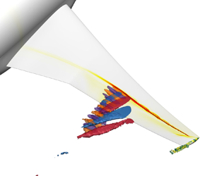
Figure 3. Real part of unsteady surface pressure coefficient ( $\hat {C}_P$) and volumetric isosurfaces of the real part of the
  $x$-momentum perturbation
  $\hat {\rho u}$ at values
  ${\pm }1.5$ showing optimal responses at angle of attack
  $\alpha = 3.5^\circ$ for (a) the long wavelength mode at angular frequency
  $\omega =0.164$, (b) the buffet mode at
  $\omega =3.33$, (c) the wake mode at
  $\omega =19.3$ and (d) the wingtip mode at
  $\omega =51.8$. Underlying vectors are scaled to unit length with respect to the volume-weighted inner product,
  $\langle \hat {\boldsymbol {w}},\hat {\boldsymbol {w}}\rangle = 1$. The base-flow zero-skin-friction line is also shown on the surface. To aid the interpretation of the slices shown in figures 4 through 6, the dimensionless span locations
  $\eta$ are included for long wavelength, buffet and wake modes.
Similar observations about the gain of the buffet and wake modes were previously made in the aerofoil study by Reference Sartor, Mettot and SippSartor et al. (2015), albeit obviously identifying the aerofoil buffet mode rather than the finite-wing buffet modes. Comparing with the aerofoil study in Reference Moise, Zauner, Sandham, Timme and HeMoise, Zauner, Sandham, Timme, and He (in press) shows that modal analysis of data from large-eddy simulations offers similar conclusions within the limits of the underlying modelling assumptions of the different flow models. Speaking of the aerofoil mode, some very weak bumps for angular frequencies  $\omega <1$ can be observed in the same figure 2(b), too. To understand better if we are indeed looking at the finite wing equivalent of the aerofoil-type mode that was also identified in the infinite-wing studies (Reference Crouch, Garbaruk and StreletsCrouch et al., 2019; Reference He and TimmeHe & Timme, 2021; Reference Paladini, Beneddine, Dandois, Sipp and RobinetPaladini et al., 2019), we scrutinised the wavemaker coefficient and the ratio of the two leading singular values,
  $\sigma _1/\sigma _2$, shown in figures 2(c) and 2(d), respectively. We focus on angle of attack
  $\alpha =3.5^\circ$. Interestingly, the wavemaker coefficient defined in (2.8) reveals four clear peaks previously contemplated through the energy gain. Besides the finite-wing buffet and wingtip vortex modal behaviour, the peaks around
  $\omega =0.2$ and
  $20$ are now more pronounced. Finite-wing buffet remains the dominant mechanism. Similar conclusions can be drawn from figure 2(d) showing the ratio. A higher ratio indicates a stronger influence of the leading mode. From a numerical point of view, well-separated singular values are beneficial for the iterative resolvent method to converge rapidly (Reference House, Skene, Ribeiro, Yeh and TairaHouse, Skene, Ribeiro, Yeh, & Taira, 2022). The somewhat erratic behaviour around the wake mode frequencies was found to be linked to competing leading modes and mode switching, but this is not further discussed herein. All four peaks correspond to distinct physics with coherent spatial structures, as discussed next.
Figures 3 through 6 offer a glimpse into the spatial characteristics of the optimal forcing and response modes at angle of attack  $\alpha =3.5^\circ$ and a few selected frequencies corresponding to distinct features discussed earlier. In figure 3 the response modes can be seen for the four angular frequencies
  $\omega = 0.164$,
  $3.33$,
  $19.3$ and
  $51.8$ showing the real part of the perturbation in the surface pressure coefficient as well as volumetric isosurfaces of the real part of the
  $x$-momentum component
  $\hat {\rho u}$. Starting with the angular frequency
  $\omega = 3.33$, which corresponds to the global peak in the energy gain at this angle of attack, the response mode, shown in figures 3(b) and 5(a), reveals a strong resemblance to the finite-wing shock-buffet modes with so-called buffet cells visible aft of the shock front (Reference Houtman and TimmeHoutman & Timme, 2021; Reference TimmeTimme, 2020). Equally, the forcing mode shape, shown in figure 5(b), comes with features resembling the adjoint shock-buffet mode visualised in Reference TimmeTimme (2018). Hence, the major peak discussed in the narrative relating to figure 2 can indeed be regarded as an early indicator (at lower angles of attack) of imminent global aerodynamic instability, even though no weakly damped and, hence, distinguishable eigenmodes can be found. Furthermore, analysing the phase, specifically
  $\angle {\hat {C}_P}=\arctan ({\text {Im}(\hat {C}_P)}/{\text {Re}(\hat {C}_P)})$, this mode is shown to be outboard running, in agreement with the unstable shock-buffet eigenmode. Note that similar statements can be made for the modes at the surrounding frequencies constituting the peak and these are not explicitly shown herein. For instance, at angular frequency
  $\omega = 2.5$, which is close to the frequency of the leading eigenmode at the instability onset angle of attack, similar but coarser-grained features (effectively correlated with the forcing frequency) can be identified. The wavemaker in figure 5(c) suggests that the flow is at its most sensitive at the shock foot and its immediate downstream separation region, indicating this region is likely important to the shock-buffet dynamics. It should be noted that the wavemaker is notably absent around the base-flow shock-wave position itself, which is in contrast to the results on two-dimensional aerofoils and infinite wings (Reference Paladini, Beneddine, Dandois, Sipp and RobinetPaladini et al., 2019).
The discussion now turns to the minor bump at low frequencies, specifically angular frequency  $\omega = 0.168$. In the energy gain plot, this peak is rather subtle, but it is clearly present for the wavemaker coefficient in figure 2(c), indicating the potential for self-excitation. Inspecting the visualisation of the optimal response mode in figures 3(a) and 4(a), it can be seen that the unsteady pressure footprint of the mode has a wavelength of the order of the (semi-)span of the wing and comes with a stronger emphasis on the shock front itself. Note that the strength of the unsteady surface pressure is reduced markedly inboard of the Yehudi break at
  $37\,\%$ semi-span approximately where the two legs of the
  $\lambda$-shock pattern merge into a single shock front coinciding with the inboard extent of the base-flow reverse-flow region, cf. Reference TimmeTimme (2020) and figure 1(c). The response mode shows some resemblance to those aerofoil buffet modes and equivalent span-uniform modes found on infinite wings (Reference He and TimmeHe & Timme, 2020; Reference Paladini, Beneddine, Dandois, Sipp and RobinetPaladini et al., 2019; Reference Sartor, Mettot and SippSartor et al., 2015) and, importantly, this mode is not obtained in a global stability analysis. In this context it is also instructive to mention the long wavelength modes discussed in Reference DandoisDandois (2016) and Reference Masini, Timme and PeaceMasini, Timme, and Peace (2020) (with the latter using modal decomposition of experimental dynamic pressure-sensitive paint data in the vicinity of the actual onset condition, below and above), Reference Ohmichi, Ishida and HashimotoOhmichi, Ishida, and Hashimoto (2018) (using modal decomposition of scale-resolved numerical simulation data in an established shock-buffet regime), and Reference Sansica and HashimotoSansica and Hashimoto (2022) (using a global stability analysis also well beyond their onset point). Similar to the long wavelength aerofoil-equivalent modes in the infinite-wing studies, the direction of these spanwise modes, either inboard or outboard, is often discussed. Herein, we find a propagation direction weakly biased towards outboard that would agree with the
  $80\,\%$-scaled NASA CRM wing study in Reference Ohmichi, Ishida and HashimotoOhmichi et al. (2018), albeit, as stated earlier, being in an established shock-buffet condition. Continuing with the forcing mode and inspecting a slice shown in figure 4(b), some resemblance with the adjoint eigenmode near the shock-buffet onset angle of attack on both a two-dimensional aerofoil (Reference Sartor, Mettot and SippSartor et al., 2015) and a three-dimensional infinite wing (Reference He and TimmeHe & Timme, 2020) can also be noted. Of course, herein we are dealing with a three-dimensional finite wing and, hence, variation in the span direction must be taken into account. A prominent feature is the oblique line impinging on the shock-foot location, where the boundary layer separates and the spatial amplitudes of opposite sign along the wall shear layer are parallel to the wing surface. It was demonstrated that this oblique part of the forcing mode coincides with a right characteristic line within the supersonic region, emphasising the importance to the whole dynamics of the shock-wave/boundary-layer interaction. The reader is referred to Reference Sartor, Mettot and SippSartor et al. (2015) for more discussion on this point. The wavemaker for this mode shown in figure 4(c), similarly to the wavemaker of the finite-wing buffet mode in figure 5(c), highlights the shock foot and immediate separation region, albeit over a smaller spanwise extent and at a more inboard location. Although the response mode exhibits unsteady pressure fluctuations on the entire shock foot along the (semi-)span, the overlap with the forcing mode is rather small as shown in the wavemaker. Carefully interpreting the wavemaker coefficient in figure 2(c), too, the results could potentially point towards the elusive equivalent of an aerofoil (or long wavelength) mode on a finite wing, albeit subdued due to more complex geometric features, including taper, twist, sweep and, of course, finite aspect ratio, and resulting localisation of the reverse-flow region that then is in stark contrast to the description of the proper aerofoil mode.

Figure 4. Long wavelength mode at angle of attack  $\alpha =3.5^\circ$ showing the real part of the
  $x$-momentum component
  $\hat {\rho u}$ for (a) the response at
  $\eta =0.61$, (b) the forcing at
  $\eta =0.51$ and (c) the momentum-only resolvent wavemaker. Inset of wavemaker plot shows three isosurfaces at values
  $\theta = 1\times 10^5$,
  $5\times 10^5$ and
  $1\times 10^6$. The sonic and zero-skin-friction lines are also shown.

Figure 5. Buffet mode at angle of attack  $\alpha =3.5^\circ$ showing the real part of the
  $x$-momentum component
  $\hat {\rho u}$ for (a) the response at
  $\eta =0.62$, (b) the forcing at
  $\eta =0.5$ and (c) the momentum-only resolvent wavemaker. Inset of wavemaker plot shows three isosurfaces at values
  $\theta = 1\times 10^5$,
  $5\times 10^5$ and
  $1\times 10^6$. The sonic and zero-skin-friction lines are also shown.
The bump at angular frequency  $\omega = 19.3$ is discussed next. This mode, shown in figures 3(c) and 6, corresponds to a wake mode, extensively discussed in Reference Sartor, Mettot and SippSartor et al. (2015) and Reference Moise, Zauner and SandhamMoise et al. (2022). The unsteady wake manifests itself over the same spatial region as the coherent structures of the finite-wing buffet modes, emanating from the separation region behind the shock foot, resulting in downstream vortex shedding. It is interesting to observe that its coherent flow structures are aligned approximately parallel to the wing trailing edge, which is in contrast to the inclined appearance of the buffet cells that have an outboard plus downstream direction. Once again, this mode is not found with a global stability analysis, and indeed it is often reported that the wake dynamics is likewise not captured in time-marching simulations within the unsteady Reynolds-averaged Navier–Stokes framework (Reference Moise, Zauner, Sandham, Timme and HeMoise et al., in press). The corresponding forcing mode shows a fine-grained structure over the top surface of the wing. Similarly to the previous two modes, the wavemaker is strongest in the separation region behind the shock foot, whilst also extending over a longer region in the chordwise direction, albeit only along the boundary layer. As shown in the inset, the wavemaker extends well upstream of the shock front almost reaching the wing leading edge, contrary to the aerofoil and buffet modes. The extent of the wavemaker is also more localised in the spanwise direction when compared with the aerofoil and buffet modes.

Figure 6. Wake mode at angle of attack  $\alpha =3.5^\circ$ showing the real part of the
  $x$-momentum component
  $\hat {\rho u}$ for (a) the response at
  $\eta =0.57$, (b) the forcing at
  $\eta =0.57$ and (c) the momentum-only resolvent wavemaker. Inset of wavemaker plot shows three isosurfaces at values
  $\theta = 1\times 10^5$,
  $5\times 10^5$ and
  $1\times 10^6$. The sonic and zero-skin-friction lines are also shown.
Lastly, the peak at angular frequency  $\omega = 51.3$, clearly present at all angles of attack, corresponds to a wingtip vortex mode, as can be seen in figure 3. Although the spatial characteristics of the response mode are shown for completeness, since this mode is unlikely to be important to the shock-buffet dynamics, being the focus of this study, a discussion on the response and forcing modes is omitted. It is briefly noted that, unsurprisingly, the corresponding wavemaker is therefore strongest at the wingtip.
5. Conclusions
Continuing from previous triglobal stability studies, resolvent analysis is discussed herein to further elucidate the modal nature of the finite-wing shock-buffet phenomenon that can limit the flight envelope. The size and complexity of the target application, specifically a contemporary large aircraft model, and resulting big fluid meshes for the high-Reynolds-number transonic flow, rule out the use of matrix-forming solution methods with direct matrix factorisation. Instead, by approximating the underlying SVD of the resolvent operator, a measure can be given to the optimal energy increase at a given frequency together with obtaining the pair of optimal forcing and response modes. This approximation is accomplished through an iterative method, that has been implemented in the industrial DLR-TAU code. The iterative method relies on the robust solution of large sparse linear systems of equations achieved through using an advanced preconditioned Krylov subspace iterative solver. By harmonically forcing an otherwise globally stable (or marginally unstable) system, the optimal energy gain is computed, alongside the respective forcing and response modes. Deflation of converged optimal forcing modes gives access to additional sub-optimal modes, which is useful when the engineers’ interest is in complex physical phenomena such as shock buffet.
The NASA CRM served as the test case at a free-stream Mach number of 0.85 and a chord Reynolds number of  $5\times 10^6$ according to a previous experimental test entry. The assumed rigid (yet statically deformed) case describes a fluid-only aerodynamic problem, that is discussed at four angles of attack, below the onset of large-scale unsteadiness and just above. The resolvent approach is shown to be capable of predicting strong modal behaviour, such as that linked to large-scale transonic flow unsteadiness, well before the instability onset (up to half a degree in angle of attack in our study) when a global stability tool can first identify dominant coherent physics through weakly damped eigenmodes. For the lowest angle of attack, the non-normality of the Jacobian operator is insufficient to cause a significant peak in the energy gain in the range of typical shock-buffet frequencies. This observation changes with increasing angle of attack approaching the critical value, as the typical broadband behaviour is identified. The spatial structures of the underlying optimal forcing and response modes show clear similarities with those of the respective adjoint and direct eigenvectors of the leading buffet modes found through global stability analysis at angles of attack closer to critical conditions. The corresponding resolvent wavemaker, similar in its meaning to the eigenvalue-based wavemaker in indicating the best regions for localised feedback, points towards the shock foot and the immediate downstream separated shear layer as likely important to the global dynamics. Additionally, our study reveals, besides rather interesting wingtip vortex modes, also those wake modes that are not typically observed in the framework of unsteady Reynolds-averaged Navier–Stokes simulations and another weak modal behaviour that resembles to some extent the span-uniform (aerofoil) mode identified in previous infinite-wing studies but remained elusive in near-onset finite-wing global stability analyses.
Appendix A. Assessment of iterative resolvent algorithm
The numerical characteristics of the iterative resolvent algorithm are scrutinised in figures 7 through 9; a representative convergence history of the optimal and first sub-optimal singular solutions, using the same aircraft test case at angle of attack  $\alpha =3.5^\circ$ discussed in § 4, is shown in figure 7. The representative angular frequency was chosen as
  $\omega =2.5$, approximately coinciding with the frequency of the global instability occurring near the angle of attack of onset,
  $\alpha =3.7^\circ$ but remaining below the peak in the energy gain at
  $\alpha =3.5^\circ$, as seen in figure 2(b). This choice ensures rapid convergence of the optimal solution since
  $\sigma _1/\sigma _2\gg 1.0$, as seen in figure 2(d). Even though the second sub-optimal solution was not computed, the slow convergence of the first sub-optimal solution, seen in the figure, suggests that the separation of modes is not strong (
 $\sigma _2/\sigma _3\gtrsim 1.0$). In other words, when strong modal behaviour is present in the system dynamics, the iterative resolvent method is very efficient. For modes that are harder to distinguish in their dominance, convergence can take significantly longer. For such scenarios, when, for instance, no clear winning mode is present or pairs of modes can be found (such as a pair representing port/starboard wings on a full-span aircraft configuration), an Arnoldi method could be explored in the future to enhance convergence rates (Reference Barkley, Blackburn and SherwinBarkley, Blackburn, & Sherwin, 2008; Reference Bugeat, Chassaing, Robinet and SagautBugeat, Chassaing, Robinet, & Sagaut, 2019; Reference Qadri and SchmidQadri & Schmid, 2017). Overall, our results in terms of required iterations for reaching convergence agree nicely with what was stated in Reference Gómez, Sharma and BlackburnGómez et al. (2016) or Reference House, Skene, Ribeiro, Yeh and TairaHouse et al. (2022).

Figure 7. Representative numerical behaviour of iterative resolvent method at angle of attack  $\alpha =3.5^\circ$ showing convergence of (a) singular values and (b) the flow response for optimal and first sub-optimal modes at angular frequency
  $\omega = 2.5$.
The spatial characteristics of the forcing and response modes for the optimal solution obtained at the first two iterations of the resolvent algorithm can be seen in figure 8. Specifically, the  $x$-momentum component at selected spanwise locations is shown. All mode shapes at subsequent iterations, including those at full convergence, are visually identical to the naked eye to those shown at the second iteration (at these chosen slice locations and plotting styles). To be clear, what is visualised in the figure are the right-hand side vectors for either the forward (forcing) or adjoint (response) linear systems of equations in algorithm . Even when an entirely random forcing is applied, the resulting response already shows a strong resemblance to the fully converged response mode that would emerge from an optimal forcing. This demonstrates that the resolvent operator filters the dominant dynamics rapidly, depending on the ratio of the singular values,
  $\sigma _1/\sigma _2$, even without preconditioning the initial forcing field through, e.g. an appropriate gradient weighting to incorporate information from the base flow (Reference Ribeiro, Yeh and TairaRibeiro et al., 2020). Indeed, in our case the strong shock wave comes with significant gradients in the base-flow variables whereas the optimal forcing shows almost no activity around that location. Nevertheless, a smarter, physics-informed selection of the initialisation can be considered in the future.

Figure 8. Convergence of (a,c) forcing and (b,d) response modes for a dominant singular value at angle of attack  $\alpha =3.5^\circ$ and angular frequency
  $\omega = 2.5$, at (a,b) iteration 1 and (c,d) iteration 2. The slices show the real part of the
  $x$-momentum component
  $\hat {\rho u}$ at dimensionless span locations
  $\eta = 0.52$ and
  $0.63$ for the forcing and response modes, respectively. The base-flow sonic line is also shown.
The impact of the specified convergence tolerance of the inner linear solver on the rate of convergence of the resolvent solution is presented in figure 9. The convergence of the forcing mode, in figure 9(a), is shown for different values of the factor  $\delta$, specifically
  $\delta =10^{-3}$,
  $10^{-4}$,
  $10^{-5}$ and
  $10^{-6}$. This factor indicates the inner linear solver tolerance relative to the norm of the latest solution update, specifically the forcing vector (cf. line 10 in algorithm ). For the first two iterations, reaching a level of approximately
  $10^{-5}$ using the measure
  $|1-\langle \boldsymbol {f}^j,\boldsymbol {f}^{(j-1)} \rangle |$, the convergence histories are almost identical. From there on, however, the benefits of a deeper converging inner solver become visible; the outer resolvent solution converges more quickly. Down to a tolerance of
  $10^{-9}$, that terminates the resolvent iterations, the more relaxed inner convergence level using
  $\delta =10^{-3}$ takes roughly twice the number of outer iterations compared with the stricter inner convergence level using
  $\delta =10^{-6}$. Obviously, the ideal choice of the factor
  $\delta$ should consider the number of iterations of the inner linear solver to reach those respective levels of convergence recognising that matrix-vector products with the Jacobian operator and orthogonalisation of the Krylov subspace account for the highest cost of the linear equation solver. Figure 9(b) attempts to visualise this connection for the case
  $\delta =10^{-5}$ (which is the value of
  $\delta$ used for the majority of simulations in this work). To clarify, what is shown in the figure is the relative residual norm over the linear solver iterations for both the direct and adjoint equations for all outer iterations of the resolvent algorithm until convergence. Line thickness is used to distinguish between individual linear solutions. The slower converging group corresponds to the adjoint solutions. The figure reveals three interesting aspects. First, obviously, deeper convergence levels (linked to the norm of the outer solution updates through the factor
  $\delta$) require more iterations. Second, following the first outer resolvent iteration, the inner linear solution histories are almost identical, except the additional iterations needed to reach deeper and deeper convergence depending on the outer solution level. Even though not attempted as part of this study, the results suggest that initialising the direct and adjoint solution vectors from the solutions of the previous outer iteration and using a suitable Krylov iterative method that allows subspace recycling for subsequent linear systems, such as our chosen GCRO-DR solver (Reference Xu, Timme and BadcockXu et al., 2016), can reduce the required number of inner iterations dramatically. Third, it should be noted that the final adjoint solution stalls at low residual levels, even though this does not affect the resolvent solution to converge. Since similar behaviour was observed for all values of
  $\delta$ during the final adjoint solution, we caution that continued development of robust preconditioned Krylov subspace iterative methods is needed.

Figure 9. Convergence behaviour of approximate iterative solution approach with varying factor  $\delta$ (indicating inner linear solver tolerance relative to norm of solution update), showing (a) convergence of forcing mode and (b) convergence history of inner iterations for
  $\delta =10^{-5}$. Symbols in (b) distinguish between direct (circle) and adjoint (triangle) equations, and decreasing line thickness indicates deeper linear solution tolerances.

Figure 10. Circular cylinder test case showing (a) streamwise and (b) cross-stream velocity components of the base flow. The perturbation solutions show the real part of the cross-stream velocity component,  $\hat {w}$, for leading (c) adjoint and (d) direct eigenmodes and optimal (e) forcing and (f) response modes. Also in (a) the recirculation region based on zero streamwise velocity is indicated.
Appendix B. Circular cylinder
The ubiquitous test case of a circular cylinder at a subcritical Reynolds number has been considered while implementing and verifying the methods discussed in this work. The laminar cylinder flow is discussed at a Reynolds number of  $Re=40$ (and low Mach number of
  $M=0.2$). For demonstration purposes, a rather coarse mesh with just under
  $10\,000$ control volumes is used with the domain extending to a far-field boundary of 100 cylinder diameters. The convergence tolerance is set to
  $10^{-12}$ throughout both for nonlinear iterations of the state-steady computation and the linear systems arising from the linearised aerodynamics methods. The base flow as a steady solution of the Navier–Stokes equations is given in figure 10(a,b) showing streamwise and cross-stream velocity components. Stability analysis (both the direct/right and adjoint/left calculation) predicts the leading mode (least damped) with an eigenvalue of
  $\lambda =-0.0275 +{\rm i} 0.7145$, which eventually develops into the vortex shedding instability at the critical Reynolds number of approximately
  $Re=47\unicode{x2013}48$. The corresponding eigenfunctions of the cross-stream velocity component are shown in figure 10(c,d) for the adjoint and direct modes. The underlying eigenvectors in conservative variables were scaled to unit length with respect to the volume-weighted inner product before further post-processing for visualisation. Results are consistent with published results in the literature (Reference Giannetti and LuchiniGiannetti & Luchini, 2007; Reference Sipp and LebedevSipp & Lebedev, 2007). The resolvent analysis is done for a frequency
  $\omega =0.7$, close to the critical frequency of the Hopf bifurcation, and the three leading optimal and sub-optimal modes are computed. The three singular values of those modes are
  $\sigma _1=2158.98$,
  $\sigma _2=162.66$ and
  $\sigma _3=153.86$. For debugging purposes, these calculations were also done using both Matlab functions to compute the largest eigenvalues of
  $\boldsymbol{\mathsf{RR}}^{\dagger}$ and the iterative method, described in algorithm . The TAU implementation gives identical results while also testing parallel processing on different numbers of hardware cores. The first optimal forcing and response modes are shown in figure 10(e,f). The resemblance but not perfect agreement with the eigenmodes is expected due to the frequency proximity (Reference Symon, Rosenberg, Dawson and McKeonSymon, Rosenberg, Dawson, & McKeon, 2018), while noting that the volume scaling ensures consistent magnitude but does not necessarily align the spatial phase.
Supplementary material
The simulation data that support the findings of this study are available from the authors upon reasonable request. The Common Research Model geometry is openly available at https://commonresearchmodel.larc.nasa.gov/.
Acknowledgements
An early version of this work was presented as Paper AIAA 2022-1329. We thank the German Aerospace Center for access to the TAU flow solver and the University of Liverpool for access to the high-performance computing system.
Funding statement
The first author is grateful to the Engineering and Physical Sciences Research Council (EPSRC) in the United Kingdom for the financial support through an Industrial CASE scholarship award (grant number 2271972 as part of EP/T517574/1) in partnership with Airbus. We also acknowledge EPSRC support through the joint grant EP/R037027/1 and EP/R037167/1.
Declaration of interests
The authors declare no conflict of interest.
Author contributions
J.H. created the research plan, ran simulations, post-processed data and wrote the manuscript. S.T. implemented the resolvent solver, ran simulations, advised on the data and edited the manuscript. A.S. advised on the resolvent method overall, proposed the deflation approach for suboptimal modes and reviewed the manuscript.


 Open access