


I
It has been hard to understand modern financial crises because they all appear different. If financial crises are always due to the vulnerability of short-term debt to runs, shouldn't we always see bank runs? Indeed, before the existence of central banks, crises were clearly triggered by bank runs. However, the presence of a central bank complicates matters, rendering a modern crisis timeline different and varied. Bank runs, if they occur at all, may happen late in the crisis. Or there could be no runs at all if, for example, a credible guarantee is issued.Footnote 1
Nowhere is this dynamic more evident than in 1930, the first year of the Great Depression. At the start of the Great Depression, there were no nationwide bank runs, and banks did not avail themselves of the discount window. Yet output dropped substantially: industrial production fell over 20 percent (we plot the monthly industrial production index in Figure 1 Panel A). As a consequence, 1930 is viewed as a puzzle. For example, Romer (Reference Romer1988) writes: ‘The primary mystery surrounding the Great Depression is why output fell so drastically in late 1929 and all of 1930’ (p. 5). Romer (Reference Romer1990) writes: ‘1930 is . . . the most puzzling year of the Great Depression’ (p. 599). And Bernanke (Reference Bernanke1983) notes in his study of the effects of bank failures on output: ‘it should be stated at the outset that my theory does not offer a complete explanation of the Great Depression (for example, nothing is said about 1929–1930)’ (p. 258).

Figure 1. Industrial production and bank loan spreads
Red vertical line denotes October 1929. Shaded area denotes 1930. Monthly data.
Source: Data sources described in Section II.
This article shows that a large part of the output drop in 1930 can be explained by bank actions: the reduction in loans and the switch to safe assets such as Treasuries, Munis, currency and bankers’ balances. We argue that banks realized the severity of economic conditions and took precautionary measures to protect against a potential fallout.
We further argue that this exemplifies a common feature of modern crises where a central bank is present. Banks reduce loans before the crisis while depositors stand pat to see what the central bank does, even if they already recognize crisis conditions. The true start of the crisis, then, can occur before any obvious indications of stress, such as bank failures. Indeed, Boyd et al. (Reference Boyd, De Nicolo and Loukoianova2009) examined the dating of crises in four crisis databases and find that large reductions (25 percent) in loan growth predicted crisis start dates. However, no threshold change in deposits has predictive power. Without observing these actions by the banking sector, modern crises may appear as idiosyncratic events without a common core element.
Our empirical strategy to ascertain the role of banks in output declines in 1930 combines state-industry-level data on output with state-level data on the banking sector. We use data from the Federal Reserve to construct state-level measures of banking sector behavior; we use historical Moody's Industrial Manuals to measure industry-level external finance dependence; we employ data from the Biennial Census of Manufactures to construct measures of state-industry level performance.
In order to identify the effect stemming from the banking sector's decision to cut back – and not from demand side effects – we use an approach along the lines of Rajan and Zingales (Reference Rajan and Zingales1998). We hand-collect firm balance sheet data reported in Moody’s Industrial Manuals from 1922 to 1928 and calculate a measure of external finance dependence. We include this measure of external dependence as a treatment intensity in a cross-sectional regression of industry output on contemporaneous changes in the state-level aggregate bank balance sheet.
We find that from 1929 to 1931, the output of industries that were more dependent on external finance is more severely affected by reductions in loans, reductions in total assets, reductions in deposits and increases in holdings of safe assets by their home state banks, allowing for both state- and industry-level fixed effects. Because of the Census data availability, our main outcome variables are output measures from 1929 to 1931. We discuss various methods to overcome this data limitation in Section III, where we show that this conclusion continues to hold if we measure the bank balance sheet changes from 1929 to 1930 only. We further demonstrate that bank failures do not account for the variation in output drops: our results still hold if we control for the share of deposits in failed banks from 1929 to 1931.
In order to provide a further sense of robustness, we report results from two additional analyses. First, we follow prior literature and show that our baseline estimates are robust to employing two instruments for the fragility of the state-level banking system. These instruments rely on the historical development of the banking system, and we discuss the specific types of endogeneity concerns they help to alleviate in Section III. Secondly, we re-estimate our main specifications using four alternative measures of industry-level external finance dependence from the recent literature. Again, we find results in line with baseline estimates, particularly for the three measures for which we have a good industry-level match.
The behavior of banks during this early stage of the Great Depression is evident from the aggregate balance sheet of the banking sector, shown in Table 1. From 1929 to 1931, banks cut back on loans by over 15 percent. They increased the share of total assets invested in safe assets by five percentage points, where safe assets are Treasuries, Munis, currency and bankers’ balances. At the same time, there was little action stemming from the household side: aggregate deposits fell by just 1.9 percent. This contrasts with a drop in deposits of 27.4 percent in the subsequent two years. Our estimates suggest that the loan reduction accounted for a substantial share of the output decline in 1929–31. Extrapolating from the cross-sectional estimates and nationwide totals in total bank loans, we estimate an approximately 30 percent drop in the three output measures.
Table 1. Aggregate balance sheet, 1929–33. Millions of USD. Levels, changes in levels and percentage change in selected balance sheet items

Source: Data from All-Bank Statistics: United States, 1896–1955.
Aggregate data on the cost of bank credit also backs up this view. In Figure 1 Panel B, we show that the spread between loan rates charged by banks and short-term Treasuries increased markedly in 1930, consistent with the view that banks sought to curtail credit. In fact, as Table 2 shows, the largest increase in this spread occurred in 1930.
Table 2. Bank loan spreads, yearly averages

Our empirical approach is close to that of Mladjan (Reference Mladjan2016) and Lee and Mezzanotti (Reference Lee and Mezzanotti2017). In both of these papers, the authors look at interactions of measures of firm dependence on external finance with bank failures to show effects on measures of economic performance. Mladjan (Reference Mladjan2016) studies the effects of bank failures on output in a panel of state-industry observations over the years 1929–33. Lee and Mezzanotti (Reference Lee and Mezzanotti2017) study a sample of 29 cities from 1929 to 1933. They also find that in locations where bank failures were high, the more financially dependent industries show reductions in the same three outcome variables we use: total output, employment and value-added. These papers use a similar external dependence measure to ours, based on Rajan and Zingales (Reference Rajan and Zingales1998). Nanda and Nicholas (Reference Nanda and Nicholas2014) use the external finance dependence measure to show that financial distress contributed to a slowdown in innovation during the Great Depression. In other related work, Benmelech et al. (Reference Benmelech, Frydman and Papanikolaou2019) employ identification stemming from differences in bond maturity to show that credit frictions played a large role in the employment drop from 1928 to 1933.
In contrast to these studies, we focus on the seemingly anomalous year of 1930. We demonstrate that the early part of the Great Depression, where bank failures were not substantial, can also be explained by the impact of the banking sector on the real economy. We argue there is a large causal impact of the contraction of bank lending on macroeconomic activity before the major bank runs of the Great Depression. Another recent paper focused on 1930: Hausman et al. (Reference Hausman, Rhode and Wieland2019) show that the contraction in 1930 was particularly pronounced for farm-intensive areas.
Finally, we place the crisis dynamics of the Great Depression in a broader context. We find that the unfolding of the Great Depression is typical of modern crises. At the start of the crisis, there was no widespread bank run, but output fell. In contrast, panics during the National Banking Era, 1863–1914, occurred near business cycle peaks. With the establishment of the Federal Reserve in 1914, banks had the opportunity to borrow from the discount window. During one of the first recessions under the watch of the newly established Fed, the recession of 1920–1, banks extensively used the Fed discount window, which was giving out loans at an attractive rate. The broad use of the Fed's discount window to avoid a panic was hailed at the time as having precluded a panic (see Gorton Reference Gorton1988). As described in Section IV, the discount window subsequently became stigmatized as the Fed tried to ensure that it was not used as a permanent funding source. Indeed, as demonstrated in Anbil (Reference Anbil2018), the stigma associated with seeking government assistance was a major consideration of depositors during the Great Depression. We hypothesize that because the use of the discount window had become stigmatized, banks mostly anticipated that they would not make use of it and instead opted to cut back on lending and tilted towards a safer portfolio.
To provide empirical evidence regarding the importance of discount window stigma, we rank Fed districts by the relative tightness of discount window lending in the pre-1929 sample. We show that our results are particularly pronounced in Fed districts that saw lower-than-median discount window borrowing in the pre-1929 period. Secondly, we compare the early stage of the Great Depression, 1929–31, with the prior recession in 1920–1. We re-estimate the same empirical specification and find that bank balance sheet changes do not account for the cross-sectional dispersion in output during the 1920–1 recession.
Our findings regarding the unfolding of the Great Depression suggest a reason for the common thread underlying all modern financial crises. Boyd et al. (Reference Boyd, De Nicolo and Loukoianova2009) show that modern crises are typically preceded by banks reducing loans. These authors examine the dating of crisis starts in the four main modern crisis databases: (1) Demirgüç-Kunt and Detragiache (Reference Demirgüç-Kunt and Detragiache2002, Reference Demirgüç-Kunt and Detragiache2005); (2) Caprio et al. (Reference Caprio, Klingebiel, Laeven, Noguera, Honohan and Laeven2005); (3) Reinhart and Rogoff (Reference Reinhart and Rogoff2008); (4) Laeven and Valencia (Reference Laeven and Valencia2008). These databases pin down the starting dates using an event methodology, usually noting some government intervention. Boyd et al. (Reference Boyd, De Nicolo and Loukoianova2009) find that large reductions in loan growth predict the crisis start dates in the four databases roughly a year before the traditional start date.
In contrast, deposit changes of similar magnitude do not predict the start dates. Depositors appear to wait, perhaps due to explicit or implicit deposit insurance. Loans are reduced significantly, but deposit reductions – meaning runs – only come later, if at all. In other words, banks realize the crisis conditions before any public signs of stress. Also related is Baron et al. (Reference Baron, Verner and Xiong2019), who argue that ‘quiet crises’ – drops in bank equity value without panics – are associated with subsequent credit contractions.
The article proceeds as follows. In the remainder of this section, we provide a brief literature review. Section II describes the data sources and the data construction process. Section III contains our main empirical results on the impact of bank decisions on manufacturing output. In Section IV, we compare crises during the National Banking Era and under the Federal Reserve. We also provide a history of the development of the discount window stigma. We conclude in Section V.
There is an enormous literature on various aspects of the Great Depression. Calomiris (Reference Calomiris1993) and Romer (Reference Romer1993) provide literature reviews. Perhaps closest to our work is Calomiris and Wilson (Reference Calomiris and Wilson2004). The authors do not focus on 1930, but they find evidence of banks shedding risk like us. Their focus is on New York City banks, where they show that in the early 1930s, banks shed risk, reducing dividends and increasing their holdings of safe assets. They argue that they provide ‘an explanation for the decline in bank capital and the increase in bank cash’ (p. 422).
Other related papers on the effects of bank failures and suspensions on output during the Great Depression include, for example, Bernanke (Reference Bernanke1983), Calomiris and Mason (Reference Calomiris and Mason2003), Benmelech et al. (Reference Benmelech, Frydman and Papanikolaou2019), Hausman et al. (Reference Hausman, Rhode and Wieland2019), Lee and Mezzanotti (Reference Lee and Mezzanotti2017), Mladjan (Reference Mladjan2016) and Nanda and Nicholas (Reference Nanda and Nicholas2014). Except for Hausman et al. (Reference Hausman, Rhode and Wieland2019), these authors do not examine 1930 separately. Further, several of these papers study the transmission of the shock to the banking system through the economy (e.g. by measuring dependence on bank financing), taking as given that there was a shock to banks. While this is perhaps more evident later in the Great Depression, after widespread runs on banks, it was less clear in 1930. Our article aims at understanding why banks shed risk early in the depression and how this contributed to economic activity.
Economists have advanced many hypotheses about the cause of the Great Depression: the stock market crash of 1929 (Mishkin Reference Mishkin1978; Romer Reference Romer1990); an autonomous drop in consumption (Temin Reference Temin1976); a dramatic increase in tariffs (Meltzer Reference Meltzer1976; Crucini and Kahn Reference Crucini and Kahn1996); debt deflation (Fisher Reference Fisher1933); and the nonmonetary effects of banking panics (Bernanke Reference Bernanke1983); Friedman and Schwartz (Reference Friedman and Schwartz1971) hypothesize that the primary cause of the US downturn between 1929 and 1933 was that monetary policy failed to offset bank-panic-induced declines in the money supply (also see Bordo et al. Reference Bordo, Erceg and Evans2000); and finally, Cole and Ohanian (Reference Cole and Ohanian1999) argue that technology regress can explain much of the drop in output. This is only a small sample of the vast literature.
‘Cause’ is not necessarily the same as ‘start’. Indeed, many papers on the ‘cause’ focus on the persistence and depth of depression, and not solely on the first year, which is why it remains somewhat of a puzzle. However, there is literature on the start of the Great Depression. Friedman and Schwartz (Reference Friedman and Schwartz1971) emphasize tight monetary policy as a cause of the initial output decline in 1930. However, this is disputed by Temin (Reference Temin1976) and Romer (Reference Romer1993). Romer (Reference Romer1990) points to uncertainty arising from the stock market crash, and Olney (Reference Olney1999) focuses on consumer debt burdens as causes of the large decline in US output before the first banking crisis. Hausman et al. (Reference Hausman, Rhode and Wieland2019) argue that falling farm prices and incomes can partly explain the severity of the drop in output in 1930.
We focus on the start of the Great Depression from the viewpoint of Boyd et al. (Reference Boyd, De Nicolo and Loukoianova2009), who noted the above pattern, namely that drops in loans of 10 or 25 percent forecast the starts of crises. This does not happen with large drops in deposits. So, we argue that despite the lack of depositor runs, bank behavior contributed to the output decline in 1930, as banks cut back on loans in favor of safe assets.
II
Our empirical results establish the importance of the banking sector in capturing the heretofore understudied first year of the Great Depression.
We use the cross-section of state-industry level data to establish the effects of bank behavior on macroeconomic outcomes. We measure variation in the aggregate banking sector balance sheet by state from 1929 to 1931 and link this to output declines in various industries in the corresponding state. To separate out the shock caused by a contraction in lending from a demand-side story (e.g. the particular state faced negative productivity shocks which drove down macroeconomic quantities as well as the demand for bank financing), we employ industry-external finance dependence as a measure of treatment intensity, following Rajan and Zingales (Reference Rajan and Zingales1998).
Our dataset combines information from three main sources: the Biennial Census of Manufactures, Moody's Industrial Manuals from 1922 to 1928 and statistics published by the Board of Governors of the Federal Reserve.
The Biennial Census of Manufactures provides biennial data disaggregated by manufacturing sector (industry) and state. These data are described in detail in Rosenbloom and Sundstrom (Reference Rosenbloom and Sundstrom1999) and available online on the author's website.Footnote 2 We use three measures of output provided in the Census of Manufactures: total wages (value added), value of production (gross output) and employment. Monthly aggregate industrial production data are from the St. Louis Fed FRED database (series INDPRO).
We collect firm-level data from Moody's Industrial Manuals from 1922 to 1928 to construct the measure of dependence on external finance. Firms are assigned to industries based on Ken French's industry classifications.Footnote 3 We collect Moody's Industrial Manuals data for all the firms in the industries captured by the Census of Manufactures. These balance sheet data form the basis of an industry-level proxy of external finance dependence, constructed after Rajan and Zingales (Reference Rajan and Zingales1998). The resulting industry-level measure is based on 1,224 firm-years.
Merging industry-level external finance dependence with the Biennial Census of Manufactures, we are left with 15 industries in 48 states and 387 observations (not all industries are present in all states.) Because the Census data are collected every two years, our regression evidence uses the change in the output measures from 1929 to 1931. The merged industries represent about three quarters of the total output captured by the Census of Manufactures.
State-year bank balance sheet data are from All-Bank Statistics: United States, 1896–1955, published by the Federal Reserve Board of Governors. With these data, we measure changes in state-level total assets, loans and deposits. We also construct a measure of the share of safe assets (‘Safeshare’), defined as the sum of Treasuries, Munis, currency and coin, and bankers’ balances, normalized by total assets. We construct this measure by combining the balance sheets of National and State commercial banks. All-Bank Statistics is also the source for bank loan and short Treasury rates.
Annual data on deposits in suspended banks are from the Federal Reserve Bulletin, September 1937, available online at the St. Louis Federal Reserve Bank FRASER database.Footnote 4
Finally, Fed district-level data on the use of the discount window are from Banking and Monetary Statistics, 1914–1941, published by the Federal Reserve Board of Governors and available online at the St. Louis Federal Reserve Bank FRASER website.Footnote 5
A key difficulty facing our empirical approach is the coarse frequency of industry-level output data and a mismatch in the timing of the three data sources. The Census of Manufactures was carried out every two years, with questionnaires sent out to respondents in January 1930 and January 1932. Therefore, our dependent variable measuring period bleeds into late 1931, where bank suspensions increased in magnitude. In contrast, the bank balance sheet data are captured annually at the end of June and discount window usage is captured at the end of the year. We discuss various methods to overcome this data limitation in Section III
For each firm-year, we calculate dependence on external funding as capital expenditures (Capex) minus lagged cash flow from operations (CFO), divided by Capex:

We lag CFO because the time t variable is unknown when capital expenditure decisions are made. We then sort the firm-year measures into ten buckets and assign integer values to each bucket. We do this to allow for potential nonlinearities in the relationship between CX and the bank measures. The industry-level measure is the firm asset-weighted sum of CX bucket values in industry i:

where i indexes industries; k indexes firms; I represents the set of all firms in industry i; and TAk total assets on the balance sheet of firm k.
The Census of Manufactures contains state-level data on the output and employment of 21 industries. In order to calculate industry finance dependence, we map individual companies from Moody's Manuals to the Census industries. We proceed as follows:
1. Start with Moody's firm-years where each firm has an associated Permno.
2. Use company Permno to match SIC codes provided by CRSP.
3. Match SIC codes to industry classifications by Ken French.Footnote 6
4. Match Ken French classified industries to Census industries.
With the industry match, we collapse firm-level finance dependence measures into an industry-level quantity. The firms in this calculation make up about a third of the entire CRSP market cap in 1928.
Table 3 shows the 15 Census industries for which we can construct a finance dependence measure and corresponding firms and firm-years in the sample. The table also shows the number of states for which we have output data in that category.
Table 3. Firm-level industry finance dependence measure

Note: Fifteen Census of Manufactures industries that are matched to firms in Moody's Manuals. CX VW refers to the main measure of industry external finance dependence, defined in Equation 2.
The 15 of 21 industries we can match to the external finance measure represent most of the output captured by the Census of Manufactures. Namely, the matched industries represent 74 percent of the employment, 67 percent of total wages and 75 percent of value of production. The total wages captured by the Census in 1929 were 4.2 billion USD. The GDP at the time was just over 100 billion USD.
The CX measure constructed in this section is not specific to bank finance. Instead, it captures dependence on all sources of external finance. However, bank lending constituted a substantial share of external finance at the time. As shown in Table 1, total bank loans in 1929 were nearly 42 billion USD. For reference, the total market cap of the 856 companies listed on the New York Stock Exchange (NYSE) was 89.7 billion USD in August 1929, as reported by McGrattan and Prescott (Reference Mcgrattan and Prescott2004).
III
The dynamics we describe are evident in the aggregate balance sheet of the banking sector. Table 1 shows the levels, changes in the levels, and percentage changes in all US banks' aggregate balance sheet items during the Great Depression (based on All-Bank Statistics: United States, 1896–1955). Corresponding to our output measures, the data are shown for 1929, 1931 and 1933.
Most interesting in the table are the categories that show large increases and large declines from 1929 to 1931. Total loans, loans for securities and all other loans show large declines. Safe assets, including Treasuries, Munis, cash and bankers’ balances, show substantial increases. These changes are consistent with the findings of Calomiris and Wilson (Reference Calomiris and Wilson2004), who focus on New York City, the most important banking center in the US. They show that during 1930, total loans divided by cash plus Treasuries declined 81 percent. This was primarily due to loans declining and safe assets increasing. Note that total deposits only declined by 1.9 percent in 1929–31 – the big declines in deposits started in 1932. The time-series behavior of these aggregates is shown in Figure 2.

Figure 2. Total borrowings of depository institutions from the Federal Reserve. Deposits at suspended banks. Bank balance sheet variables. State output measures
Source: Data sources described in Section II.
Our empirical analysis aims to measure the impact of changes in the various bank balance sheet items on contemporaneous output measures. Specifically, our regressions take the form,

where the outcome variable is defined as

for value-added, gross output and total employment of industry i in state s. In our baseline regressions, we weight observations by total assets of all banks in the state.
Similarly, the right-hand-side banking measures Banks are defined as

except for Safeshare, which is measured as a percentage point change. We show the aggregate time-series behavior of the output measures in Figure 2.
The variable CX VWi is an industry-level measure of external finance dependence, constructed in Section II.3. The terms αi are industry-level fixed effects, and the terms βs are state-level fixed effects. The specification does not include time-fixed effects because the regression is a pure cross-section.
By studying the interaction term of the state-level bank measure with the industry-level external finance dependence index, we can alleviate concerns about reverse causality. The underlying assumption is that in a given state, the output in industries with different exposures to external finance would have shrunk at the same rate – relative to the corresponding industry-wide averages – without the shock from the banking sector. Because the states differ in the magnitude of the banking sector shocks, we can identify the effect on output stemming from the shock to external finance availability – and not the effect from the demand side. Put differently, our empirical approach requires that the measure of external finance dependence is not correlated with the exposure of the industry to consumption shocks, or any other demand-side determinants of loan quantities. Note that we cannot include the CX VWi and ΔBanks terms separately because of the full slate of state- and industry-level fixed effects.
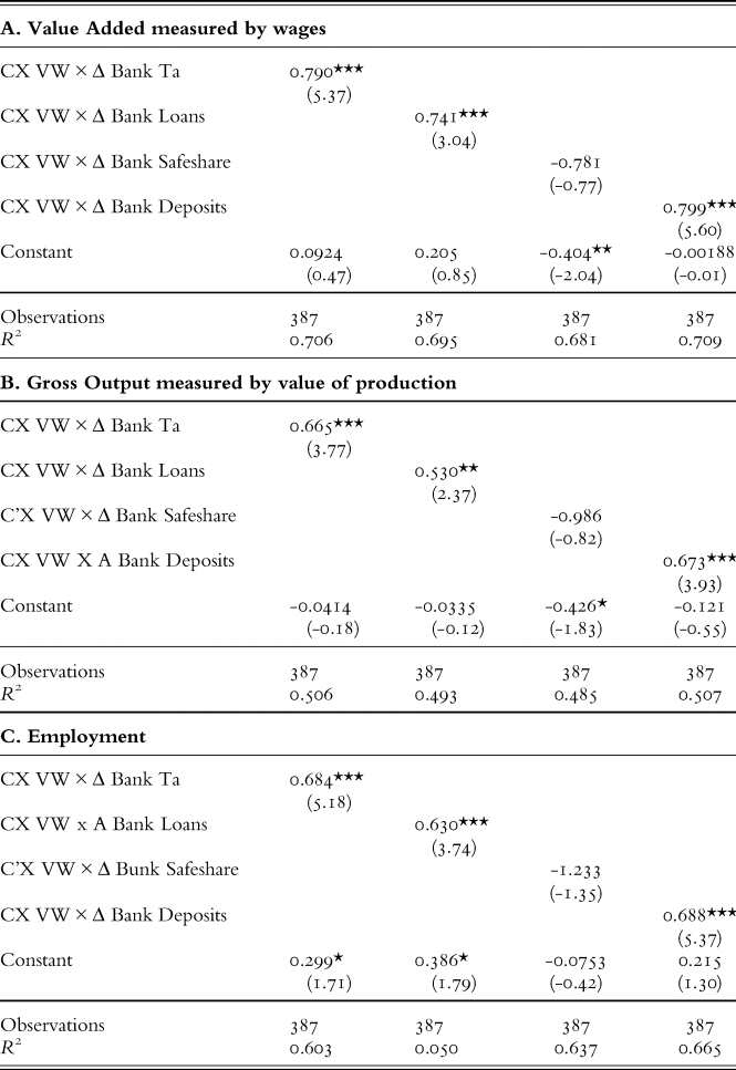
The baseline regression results are shown in Table 4. Panel A examines value added as measured by wages from 1929 to 1931. Panel B repeats the analysis with gross output as the dependent variable. Panel C repeats the same analysis with employment. In all three panels, reductions in total loans and total assets are associated with decreases in the output measures, and this relationship is statistically significant in all cases. In the specifications with value-added and employment as the dependent variable, an increase in average Safeshare in the state is a statistically significant covariate of output changes.
Table 4. OLS regressions, 1929-31

Note: Sample consists of 387 state-industry observations. Left-hand-side variable measured as a log change from 1929 to 1931. ***, ** and * denote significance at the 1%, 5% and 10% levels.
In order to put the estimated magnitudes in context, we calculate the output drop implied by the estimated coefficients of an industry with median exposure to external finance (meaning CX = 5) facing a banking sector whose balance sheet mirrors the national aggregate change. This calculation is provided in Table 5. In the table, ‘Implied aggregate’ refers to the aggregate change in the right-hand side variable under these assumptions. While all four bank balance sheet measures are estimated to have a strong impact on output, the cutback in loans was the deepest, implying the largest output loss, with estimates ranging from 27 to 44 percent.
Table 5. Interpretation of coefficients

Note: SD is the sample standard deviation of output measure, or the bank balance sheet measure. BS drop refers to the change in the total balance sheet item, as reported in Table 1. Implied aggregate measures the implied drop in output assuming an industry with median dependence on bank finance (CX=5) facing a banking sector that mirrors the change on the national level.
We now discuss the robustness of our main finding in Table 4. The first set of potential issues concerns the timing of the output measures. As discussed in Section II, the Census of Manufactures was carried out every two years, limiting us to studying industry-level output from 1929 to 1931. The inclusion of late 1931 is potentially problematic as this period saw the first nationwide banking crisis during the Great Depression era. We seek to demonstrate that including late 1931 is unlikely to drive our results by multiple robustness checks.
Firstly, we re-estimate the regressions by using bank balance sheet measures from 1929 to 1930. These results are reported in Table 6. Except for specifications with Safeshare, the results are practically identical to those reported with the two-year change in bank balance sheet measures. That is, we find that the drop in bank total assets, bank loans and bank deposits in 1929–30 are significant determinants of the drop in 1929–31 output measures.
Table 6. WLS regressions, 1929–30
Note: Right-hand-side variables measured from 1929 to 1930.
***, ** and * denote significance at the 1%, 5% and 10% levels.
Secondly, we include the share of deposits in failed banks as a control variable in our main regressions. Existing work in Mladjan (Reference Mladjan2016) has shown that suspended deposits are a strong determinant of output contraction over the entire Great Depression era. In keeping with the other right-hand-side variables, we calculate the state-level two-year change in suspended deposits and interact it with the industry-level external finance dependence measure. The results in Table 7 show that bank balance sheet variables continue to be strong determinants of industry output when controlling for deposits in suspended banks. We conclude that our results are not likely to be driven by the inclusion of late 1931.
Table 7. WLS regressions, 1929–31

Note: Controlling for change in deposits at suspended banks, normalized by total assets in 1929. ***, ** and * denote significance at the 1%, 5% and 10% levels.
The second set of potential issues concerns identification. As the Section I discusses, our primary source of identifying variation is the industry-level external finance dependence. However, any demand-side shock proportional to this dependence could have caused the changes in bank balance sheet measures. While it is tough to rule out this possibility entirely, existing literature has sought to alleviate this concern by instrumenting for the fragility of the financial sector. We follow Mladjan (Reference Mladjan2016) and use two such measures:
1. Percentage of state's bank offices that belong to branch banks in 1920.
2. Growth of farmland value in the 1910s.
Both instruments use the history of a given state's banking system to measure its ability to absorb shocks, including those brought on by the onset of the Great Depression. Because higher degrees of branching imply better risk-sharing, a higher share of branching implies a more resilient banking sector. Because higher growth in farmland value in the 1910s, on average, increased banks’ exposure to real estate, the states with higher farmland value growth in the 1910s experienced a more severe downturn in agricultural land value in the 1920s, leading to less resilient bank balance sheets. (Lee and Mezzanotti (Reference Lee and Mezzanotti2017) also use this instrument and note that it predicted bank suspensions in 1930–3.) The exclusion restriction for both instruments is that the relative growth rates of industries with different external finance dependence are uncorrelated with the sources of bank fragility.
For the IV analysis we multiply these two measures by the industry-level external finance dependence measure. We test that the instruments predict the bank balance sheet measures in Appendix Table A4. The results of the instrumental variables analysis reported in Table 8 are consistent with the WLS estimates presented in Table 4, with the exception of specifications with Safeshare, which are no longer statistically significant. We also report the F-statistics, which are above 25 in all cases, save for the Safeshare measure.
Table 8. IV regressions, 1929–31

Note: State-level instruments for fragility of the banking sector constructed by Mladjan (Reference Mladjan2016), described in Section III. ***, ** and * denote significance at the 1%, 5% and 10% levels.
Finally, our main estimates weight observations by total assets in each state's banking sector. In Table 9, we re-estimate the regressions in an OLS setting. We find a smaller implied response to the bank balance sheet variables, suggesting that the effect we document stems mostly from large states.
Table 9. OLS regressions, 1929–31

Note: Sample consists of 387 state-industry observations. ***, ** and * denote significance at the 1%, 5% and 10% levels.
In addition to our industry-level finance dependence measure described in Section II, we collect four alternative proxies of industry-level external finance dependence to establish robustness of the main findings.
1. The first alternative is the measure of credit difficulty constructed in Janas (Reference Janas2023) labeled DIFFICULTY. This variable is based on a 1935 Commerce Department survey of credit conditions, and the industry-level measure is the share of manufacturers reporting difficulty obtaining credit. We match industries to the Census classifications, and the match is shown in Appendix Table A2.
2. The second alternative measure is bank loans payable over fixed assets (LOANSFA) as constructed by Nanda and Nicholas (Reference Nanda and Nicholas2014). The raw industry-level data are reported in Table A3 of that paper. We again match industries and report the match in Appendix Table A2.
3. The third and fourth alternative measures are constructed in Mladjan (Reference Mladjan2016) and reported in Table 2 of that paper. External Dependence (ED) is a Rajan–Zingales type of measure like the one used in this article but estimated using Compustat data from 1950–2007, and rescaled to set the median to zero and maximum to one. Inverse Interest Cover (IIC) is constructed using industry-level data from IRS Statistics of Income reports in 1922–8. It equals the ratio of earnings before interest and taxes to total interest expense. The measure is again rescaled to set the median to zero and maximum to one and inverted to make it directionally comparable to the other measures. The industries for these two measures are the same as in our data.
The industry matches and dependence measure values are reported in Panel A of Table A2. Despite differences in industry definitions and coverage, we find a positive pairwise correlation between most of these alternative measures of external finance dependence. As reported in Panel B of Table A2, the pairwise correlations are positive except for the LOANSFA correlation with ED and IIC.
Table 11 presents an abbreviated version of our main analysis using these four alternative proxies for external finance dependence. We use changes in bank loans multiplied by each of the four respective external finance dependence measures as the right-hand-side variables. For three of the four proxies – DIFFICULTY, ED, IIC – we find results well in line with the baseline estimates reported in Table 4. We normalize the dependence measures to have standard deviation of one, making them directly comparable with the coefficients in Table 4 as the standard deviation of CX VW is close to one as well. We find the overall sensitivity with the alternative measures is slightly lower but in the same order of magnitude as in regressions reported in Table 4: the remaining measure, LOANSFA, results in estimates not statistically significantly different from zero. Part of the reason might be the poorer match with the Census of Manufactures industry mappings, with multiple Census industries mapped onto the same LOANSFA industry, also reflected in the smaller number of observations in these specifications. Overall, we find that the regressions employing alternative dependence measures confirm the results from the main analysis.
Table 11. WLS Regressions, 1929–31
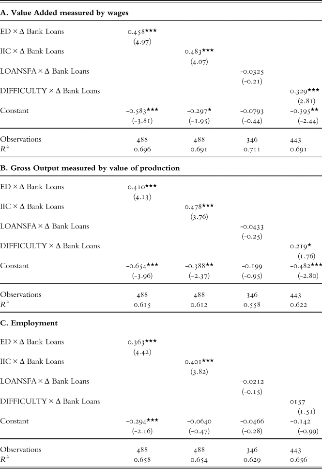
Note: Alternative measures of finance dependence on the right-hand side. Sample sizes differ due to varying industry coverage of alternative measures. ***, ** and * denote significance at the 1%, 5% and 10% levels.
As shown in Figure 2, banks made little use of the discount window in 1929–31. Instead, they opted to cut back on lending. The regression evidence suggests that the decision to cut back on lending strongly impacted economic output.
In order to illustrate the importance of the decision not to go to the discount window, we repeat the analysis presented in Table 4 for the 1920–1 recession. According to the NBER, this recession started in January 1920; the trough was July 1921. Unlike during the Great Depression, the discount rate offered by the Fed was below market rates. As a result, and in direct contrast to the Great Depression, banks extensively used the Fed's discount window during the Recession of 1920–1. As we report in Table 10, the four measures of bank balance sheet changes have little explanatory power over industry-level outcomes. Of course, these regressions assume that the external finance dependence we estimated in the 1922–8 sample also applies to the prior period. Appendix Table A1 shows the evolution of the aggregate bank balance sheet during the 1920–1 recession. We interpret this as evidence of the importance of discount window stigma during the Great Depression. Section IV provides a narrative account of the Fed's attempt to introduce a discount window stigma after the 1920–1 recession.
Table 10. WLS regressions, 1919–21

Note: Sample consists of 387 state-industry observations. Left-hand-side variable measured as a log change from 1929 to 1931. ***, ** and * denote significance at the 1%, 5% and 10% levels.
To provide further evidence that the discount window stigma contributed to banks’ decision-making in 1929–31, we seek to exploit the feature that discount window conditions were set separately by each Fed district. Richardson and Troost (Reference Richardson and Troost2009) document that districts differed in the tightness of discount window borrowing.Footnote 7 In order to capture local discount window tightness, we calculate the average share of discount window borrowing to total bank assets in a given year. We then rank Fed districts yearly and calculate the average annual rank from 1915 to 1928. We interpret this rank as a measure of a given Fed district's discount window strictness.
We then re-estimate the baseline regressions by including a dummy variable for states predominantly in Fed districts below the median in discount window borrowing intensity from 1915 to 1928. Appendix Table A5 shows that our baseline results are particularly pronounced in states where discount window borrowing was tight before 1929. The triple interaction term of bank balance sheet measure with finance dependence with low discount window usage is responsible for most output dependence on bank balance sheet measures.
Of course, this does not establish causality from discount window strictness to output changes in 1929–31. However, we consider this suggestive evidence favoring the view that discount window stigma was paramount.
IV
As discussed, the lack of discount window borrowing in the early part of the Great Depression stands in contrast to the recession of 1920–1. This section summarizes the history of earlier banking panics in the US. Then, we provide a brief history of the Federal Reserve's discount window policy and the development of stigma. The main contrast to bank panics in the National Banking Era is that panics had previously been more strongly tied to business cycle turning points – they regularly occurred shortly after signals of an economic downturn, as shown in Gorton (Reference Gorton1988).
The National Banking Era began with legislation in 1863 that introduced a system of ‘national banks’ that could issue their own currency but required backing by US Treasuries. The legislation aimed to develop a demand for US Treasuries to finance the North in the Civil War. But, in addition, it was thought that with Treasury backing, creating a uniform currency (i.e. one without discounts from face value as had occurred with private bank money prior to the Civil War), there would no longer be banking panics – which did not turn out to be the case. In the National Banking Era panics depositors sought to withdraw their cash in National Bank notes.
Gorton (Reference Gorton1988) analyzes seven panics during this period: 1873, 1884, 1890, 1893, 1893, 1896, 1907 and 1914. These panics occurred at or just after business cycle peaks; see Gorton (Reference Gorton1988) and Calomiris and Gorton (Reference Calomiris, Gorton and Hubbard1991).Footnote 8 Gorton (Reference Gorton1988) showed that banking panics during the National Banking Era, 1863–1914, were information events. The panics occurred when depositors observed an innovation in a leading indicator of recessions: the liabilities of failed businesses.Footnote 9 If this measure exceeded a threshold, it indicated that a large recession was coming and, upon observing this information, there would be a panic. There was never a panic without this threshold being exceeded, and there was no case where the threshold was exceeded without a panic. After the Federal Reserve System came into being, this threshold can be used to determine the counterfactual of when panics could have occurred.
The purpose of the Federal Reserve System was to prevent banking panics by having a permanent discount window that banks could always access.Footnote 10
According to the measure of innovation in the liabilities of failed businesses, estimated over the period 1873–1934, two shocks exceeded the threshold: June 1920 and December 1929. These two dates follow business cycle peaks, just as in the pre-Fed period. However, there was no panic at the start of the recession of January 1920 – July 1921. Banks heavily used the discount window during the 1920–1 recession. Figure 2 shows the dramatic use of the window during the 1920 recession. The successful avoidance of a panic in 1920 was widely remarked upon at the time. For example, Herbert Hoover, then the Commerce Secretary, said, ‘We know now that we have cured [bank panics] through the Federal Reserve System.’Footnote 11 Moreover, Wesley Mitchell wrote in 1922 that: ‘We have learned how to prevent crises from degenerating into panics’ (see Mitchell Reference Mitchell1922).
At that time of the 1920–1 recession, the discount rate was below market rates because the Federal Reserve wanted to support the sale of US Treasuries to pay off the debt from World War I. Background on the Fed–Treasury relations during this period can be found in Beckhart (Reference Beckhart1924), Meltzer (Reference Meltzer2003), Parker and Steiner (Reference Parker and Steiner1926), Whittlesey (Reference Whittlesey1959) and Wicker (Reference Wicker1966, Reference Wicker2015), among others. In any case, banks did avail themselves of the discount window to a significant extent, as seen in Figure 2. However, the Fed became concerned that banks were using the discount window as a permanent source of funding and using the discount window borrowings to lend to speculative stock market investors. To solve these perceived problems, the Fed introduced the discount window stigma. To control discount window borrowing without raising the discount rate (to accommodate the Treasury), the Fed introduced non-pecuniary penalties. The methods used to control credit are listed by Parker and Steiner (Reference Parker and Steiner1926): the issuance of warnings; the use of moral suasion; advising banks to reduce their outstanding lines of credit and to discriminate against speculative and non-essential loans; the rationing of credit; the attempt to drive war paper from the portfolios of reserve member banks; controlling the issue of Federal Reserve notes; closer scrutiny of paper offered for discount.
Parker and Steiner (Reference Parker and Steiner1926) write that: ‘moral pressure was exercised by means of conferences with groups of banks and with individual banks to ascertain the reason for heavy borrowing and if necessary to request them to reduce their aggregate borrowings’ (p. 530). In the beginning of the 1920s there was less stigma. As Carlson and Duygan-Bump (Reference Carlson and Duygan-Bump2016) note: ‘There was notably less stigma associated with borrowing from the discount window in the 1920s, and borrowing was fairly widespread with about one-third of all member banks borrowing in any given month (roughly 3,000 borrowers out of 9,000 member banks)’ (no page). But, this changed, as Armantier et al. (Reference Armantier, Lee and Sarkar2015) find: ‘From the late 1920s, the DW [discount window] gradually fell into disuse as the Fed began to take a dim view of DW borrowing and adopted a stance against this practice’ (no page). Whittlesey (Reference Whittlesey1959) comments: ‘administration of the discount window, in the admonitory, moral suasion sense, has a tendency to strengthen the attitude of mind among bankers, “the instinct against borrowing,” which is the basis of the tradition [against borrowing]. To be admonished is likely to seem embarrassing and even humiliating’ (pp. 213–14).
The introduction of non-pecuniary penalties worked. Discount window borrowing declined, but with unintended consequences. Banks did not borrow from the discount window in 1929 and 1930, as in 1920–1.
Wicker (Reference Wicker1996), speaking of the localized panic in late 1930, wrote:
We can look in vain in the pages of the financial press for an event clearly designated as a panic; it was certainly not the name given to the accelerated bank suspensions in the final two months of 1930. The public had no difficulty in identifying the banking crises in 1873, 1884, 1893, and 1907. The passage of time should not have dulled the recognition of a banking crisis in 1930, especially if the events in those months bore a close resemblance to what had happened earlier. (p. 24)
Our interpretation is that banks realized they were in crisis conditions but did not go, and did not expect to be going to the discount window because of the stigma.
By the end of 1930 there were bank failures as there had been in the 1920s. However, the consensus view is that these were insignificant in turning a recession into a depression. The significant runs came later. White (Reference White1984) concludes: ‘the [1930] banking crisis did not mark the change from a recession to a depression. These results corroborate other recent studies that . . . find that the crisis [in 1930] was primarily regional in nature and had little impact on the national economy’ (p. 120); and ‘The importance of the banking crisis in 1930 in the history of the Great Depression appears to be somewhat inflated. The increased number of bank failures did not represent a radical departure from the 1920s. The characteristics of the banks that failed in 1930 were very similar to those failed in earlier years’ (p. 138). Also, Calomiris (Reference Calomiris1993): ‘the first banking crisis of 1930, may have been primarily of local importance and seems to have had little effect on national economic activity’ (p. 65). While the bank failures in late 1930 were limited, banks started to fail later during all-out panics in 1931 and 1933, as Friedman and Schwartz (Reference Friedman and Schwartz1971) described, for example.
V
The first year of the Great Depression appears to be an anomaly. Industrial output dropped by over 20 percent, but no immediate signs of banking troubles were evident. In this article, we show that the banks’ decision to significantly cut back on lending and invest instead in safe assets contributed to the drop in output. Consistent with the results of Boyd et al. (Reference Boyd, De Nicolo and Loukoianova2009), we find large loan growth declines preceding the start of the crisis. As these authors show, loan growth predicts the start dates of modern financial crises based on when the government or central bank responds. Indeed, this feature is evident in the Global Financial Crisis as well: bank loan issuance peaked in 2007Q2, well before the government action in response to Bear Stearns and Lehman Brothers’ failures in 2008 (for instance, see Panel B of Figure 1 in Ivashina and Scharfstein (Reference Ivashina and Scharfstein2010)).
This observation establishes a common thread through seemingly idiosyncratic modern financial crises. At the start of the Great Depression, depositors did not run to banks, perhaps having faith in the discount window, which was significantly used in the recession of 1920–1. In modern crises, depositors generally wait, perhaps due to explicit or implicit deposit insurance. Therefore, the economy can be in crisis conditions without apparent distress signals.
Our results are complementary to Romer (Reference Romer1990) and Olney (Reference Olney1999). Romer (Reference Romer1990) argues that the stock market crash of 1929 created ‘uncertainty’ which caused a reduction in household purchases. Similarly, the explanation in Olney (Reference Olney1999) centers on households cutting expenditures. These cuts were primarily not due to banks reducing consumer loans as banks did not make significant amounts of consumer loans until later (see Clark Reference Clark1931). With respect to Romer (Reference Romer1990), we offer a possible interpretation of this ‘uncertainty.’ Households observed the leading indicator shock and knew that they would have panicked prior to the Fed – but there was still uncertainty about whether the discount window would work. Banks, however, responded to the leading indicator by cutting lending and investing in safe assets.
Supplementary material
To view supplementary material for this article, please visit https://doi.org/10.1017/S0968565023000124


