


1. Introduction
Time decay of solutions of systems of partial differential equations is a relevant topic to be studied from the viewpoints of Mathematics and Thermomechanics. From the mathematical point of view, we would like to know estimates for the rate of decay of the solutions for a certain mathematical problem. When the system of equations describes the behaviour of a thermomechanical problem, it will be relevant to know when the perturbations can be neglected and this fact can be a consequence of the rate of decay. A situation where we can find this relevance is the study of the thermoelasticity. In fact, the time decay of solutions to thermoelastic systems has generated much literature.
To our knowledge, the first researcher who studied the thermoelastic system from a mathematical point of view was Dafermos [Reference Dafermos5]. Two relevant facts of this study were the proofs of the asymptotic stability in dimension one and the existence of isothermal undamped solutions for certain geometries of the solid (in dimension greater than one). Later, several authors obtained the exponential decay of the solutions in dimension one [Reference Lebeau and Zuazua16, Reference Muñoz-Rivera19, Reference Slemrod25] as well as the slow decay in dimension greater than one [Reference Koch15, Reference Lebeau and Zuazua16]. Some results were also obtained when the thermoelastic theory corresponds to the hyperbolic heat equation proposed by Cattaneo and Maxwell [Reference Cattaneo4] (see, for instance, [Reference Amendola and Lazzari2, Reference Racke24]). A good explanation of the results on this topic until the beginning of this century can be found in the book of Jiang and Racke [Reference Jiang and Racke14]. Some further results with other heat equations can be found in [Reference Quintanilla20, Reference Quintanilla and Racke21].
However, one fact can be concluded from all these studies. We cannot obtain exponential decay of solutions for thermoelastic problems in dimension greater than one if we only consider one dissipation mechanism. To overcome this fact, we could try to consider more than one dissipation mechanism as we can see in reference [Reference Ieşan12]. Indeed, in the recent past [Reference Fernández and Quintanilla6–Reference Fernández and Quintanilla8] we have seen how it is possible to obtain the exponential decay of the solutions if we consider
 $n^2$
-coupling mechanisms (being
$n^2$
-coupling mechanisms (being
 $n$
the dimension of the domain) in linearised elasticity. In the case when we consider the linear theory, the number of coupling mechanisms can be smaller [Reference Bazarra, Fernández and Quintanilla3]. However, it is important to point out that we always need to assume that the coupling coefficients are anisotropic.
$n$
the dimension of the domain) in linearised elasticity. In the case when we consider the linear theory, the number of coupling mechanisms can be smaller [Reference Bazarra, Fernández and Quintanilla3]. However, it is important to point out that we always need to assume that the coupling coefficients are anisotropic.
The analysis described before corresponds to the case of the usual elasticity. However, few attention has been deserved to the case of the strain gradient elasticity. We know that, in dimension one, the solutions are exponentially stable for the Fourier heat conduction in the isotropic case [Reference Fernández-Sare, Muñoz-Rivera and Quintanilla9] and that, when the heat conduction is described by the hyperbolic theories, we cannot expect a similar behaviour [Reference Quintanilla, Racke and Ueda23]. However, we do not know any study concerning time decay of the solutions for strain gradient thermoelasticity for domains with dimension greater than one. Although we do not know any proof, it is natural to expect that the decay will be slow for dimension greater than one. In view of the studies developed for the classical elasticity, we could ask about the number of the dissipative coupling mechanisms that we need to introduce to obtain exponential decay.
We want to highlight that, in the case of the strain gradient elasticity, we have spatial derivatives of fourth order, but we also have coupling terms which have spatial derivatives of second order for non-centrosymmetric materials. This stronger coupling proposed in this case allows us to see that we need only
 $n$
dissipative couplings to guarantee the exponential decay of solutions. This fact is remarkable if we recall that, in the case of the classical elasticity, the number of necessary coupling mechanisms is greater. Nevertheless, it is important to note that our results only apply in the case of Chiral materials (the materials are not centrosymmetric). Indeed, we will see that the solutions are analytic when Fourier law is used. This fact represents a strong regularity of the solutions. We will also consider the problem when the dissipation mechanisms are given by using the Green-Lindsay theory [Reference Green and Lindsay10]. In this case, we will sketch the proof of the exponential decay of solutions.
$n$
dissipative couplings to guarantee the exponential decay of solutions. This fact is remarkable if we recall that, in the case of the classical elasticity, the number of necessary coupling mechanisms is greater. Nevertheless, it is important to note that our results only apply in the case of Chiral materials (the materials are not centrosymmetric). Indeed, we will see that the solutions are analytic when Fourier law is used. This fact represents a strong regularity of the solutions. We will also consider the problem when the dissipation mechanisms are given by using the Green-Lindsay theory [Reference Green and Lindsay10]. In this case, we will sketch the proof of the exponential decay of solutions.
The plan of this paper is the following. In the next section, we propose the problem to be studied as well as the basic assumptions. In Section 3, we show that the problem is well-posed. Later, we impose a ‘relevant’ assumption on the coupling terms, which guarantees the exponential decay of the solution as we prove in Section 4. Analyticity of the solutions is proved in Section 5. Some comments about how to extend the results to the Green-Lindsay theory [Reference Lord and Shulman18] are shown in Section 6. A few comments end the paper in Section 7.
2. Basic equations and assumptions
In this section, we propose the system of equations and the basic conditions under which we are going to work in this article. We consider a two-dimensional domain
 $B$
with a boundary smooth enough (
$B$
with a boundary smooth enough (
 $C^1$
) to apply our arguments (Divergence and Trace theorems).
$C^1$
) to apply our arguments (Divergence and Trace theorems).
We assume that our domain is occupied by a homogeneousFootnote
1
strain gradient elastic material with two dissipative mechanisms that we could think as temperature (
 $\theta _1$
) and mass dissipation (
$\theta _1$
) and mass dissipation (
 $\theta _2$
).
$\theta _2$
).
Our system of equations can be written as
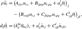 \begin{align} \rho \ddot{u}_i&=\left (A_{ijrs}u_{r,s}+B_{ijpqr}u_{r,pq}+a_{ij}^l\theta _l\right )_{,j}\nonumber \\[5pt] & \quad -\left (B_{rsijk}u_{r,s}+C_{jkipqr}u_{r,pq}+C_{ijk}^l\theta _l\right )_{,jk}\!,\\[5pt] d_{lj}\dot{\theta }_j&=(k_{ij}^{lm}\theta _{m,j})_{,i}+a_{ij}^l \dot{u}_{i,j}+C_{ijk}^l\dot{u}_{i,jk}, \nonumber \end{align}
where
 $i,j,k,m,p,q,r,s,l=1,2$
.
$i,j,k,m,p,q,r,s,l=1,2$
.
We are going to assume the initial conditions, for a.e.
 ${\boldsymbol{x}}\in B$
,
${\boldsymbol{x}}\in B$
,
 \begin{equation} u_i({\boldsymbol{x}},0)=u_i^0({\boldsymbol{x}}),\quad \dot{u}_i({\boldsymbol{x}},0)=v_i^0({\boldsymbol{x}}),\quad \theta _j({\boldsymbol{x}},0)=\theta _j^0({\boldsymbol{x}}), \end{equation}
and the boundary conditions:
 \begin{equation} u_i({\boldsymbol{x}},t)=u_{i,j}({\boldsymbol{x}},t)=\theta _i({\boldsymbol{x}},t)=0\quad{\boldsymbol{x}}\in \partial B, \,\, t\gt 0. \end{equation}
In system (2.1),
 $u_i$
is the two-dimensional displacement,
$u_i$
is the two-dimensional displacement,
 $\theta _1$
is the temperature,
$\theta _1$
is the temperature,
 $\theta _2$
is the mass dissipation variable,
$\theta _2$
is the mass dissipation variable,
 $A_{ijrs}$
,
$A_{ijrs}$
,
 $B_{ijpqr}$
and
$B_{ijpqr}$
and
 $C_{ijkpqr}$
define the strain gradient elasticity,
$C_{ijkpqr}$
define the strain gradient elasticity,
 $\rho$
is the mass density,
$\rho$
is the mass density,
 $d_{ij}$
plays a role similar to the thermal capacity in the classical heat equation, and
$d_{ij}$
plays a role similar to the thermal capacity in the classical heat equation, and
 $k_{ij}^{lm}$
has a role similar to the thermal conductivity, and
$k_{ij}^{lm}$
has a role similar to the thermal conductivity, and
 $a_{ij}^l$
and
$a_{ij}^l$
and
 $C_{ijk}^l$
are the coupling terms.
$C_{ijk}^l$
are the coupling terms.
From now on, we are going to assume that
-
(i)
 $\rho \gt 0$
,
$d_{ij}$
is a positive definite matrix.
$\rho \gt 0$
,
$d_{ij}$
is a positive definite matrix. -
(ii) There exists a positive constant
$C$
such that(2.4)for every vector function
\begin{equation} \begin{array}{l} \displaystyle \int _B\Big ( A_{ijrs}u_{i,j}u_{r,s}+2B_{ijpqr}u_{i,j}u_{r,pq}+C_{ijlpqr}u_{l,ij}u_{r,pq}\Big )\, dA\\[5pt] \qquad \displaystyle \qquad \geqslant C\int _B \Big (u_{i,j}u_{i,j}+u_{r,pq}u_{r,pq}\Big )\, dA \end{array} \end{equation}
$u_i$
vanishing on the boundary.
-
(iii) There exists a positive constant
$D$
such that(2.5)
\begin{equation} k_{ij}^{lm}\theta _{l,i}\theta _{m,j}\geqslant D \theta _{i,j}\theta _{i,j}. \end{equation}
-
(iv) The terms
$A_{ijrs}$
,
$B_{ijpqr}$
,
$C_{ijkpqr}$
,
$C_{ijk}^l$
,
$d_{ij}$
and
$k_{ij}^{lm}$
are symmetric in the sense that(2.6)
\begin{equation} \begin{array}{l} A_{ijrs}=A_{rsij},\quad B_{ijpqr}=B_{ijqpr},\quad C_{ijkpqr}=C_{jikpqr},\quad C_{ijk}^l=C_{ikj}^l,\\[5pt] d_{ij}=d_{ji},\quad k_{ij}^{lm}=k_{ji}^{ml}. \end{array} \end{equation}


We note that assumptions (i)–(iv) are natural in the study of strain gradient thermoelasticity. The meaning of (i) is obvious, the condition (ii) can be interpreted in the context of the elastic stability, condition (iii) guarantees that the dissipation is positive and conditions (iv) are also natural in the context of two dissipation mechanisms.
We are going to transform our problem as a Cauchy problem defined on a suitable Hilbert space. From now on, we denote by
 $\mathcal{H}$
the space:
$\mathcal{H}$
the space:
 \begin{equation*}\mathcal {H}={\boldsymbol{W}}_0^{2,2}(B)\times {\boldsymbol{L}}^2(B)\times {\boldsymbol{L}}^2(B),\end{equation*}
where
 ${\boldsymbol{W}}_0^{2,2}(B)=[W_0^{2,2}(B)]^2$
and
${\boldsymbol{W}}_0^{2,2}(B)=[W_0^{2,2}(B)]^2$
and
 ${\boldsymbol{L}}^2(B)=[L^2(B)]^2$
, with
${\boldsymbol{L}}^2(B)=[L^2(B)]^2$
, with
 $W_0^{2,2}(B)$
and
$W_0^{2,2}(B)$
and
 $L^2(B)$
being the usual Sobolev spaces [Reference Adams and Fournier1] (i.e. the boldface is used to define vectors). An element in our space can be determined by
$L^2(B)$
being the usual Sobolev spaces [Reference Adams and Fournier1] (i.e. the boldface is used to define vectors). An element in our space can be determined by
 $(u_1,u_2,v_1,v_2,\theta _1,\theta _2)$
. Moreover, the vector
$(u_1,u_2,v_1,v_2,\theta _1,\theta _2)$
. Moreover, the vector
 ${\boldsymbol{v}}=(v_1,v_2)$
is considered for the time derivative of the displacement vector.
${\boldsymbol{v}}=(v_1,v_2)$
is considered for the time derivative of the displacement vector.
If we consider the vector
 $({\boldsymbol{u}},{\boldsymbol{v}},{\boldsymbol{\theta }})$
, we can define the square of the norm:
$({\boldsymbol{u}},{\boldsymbol{v}},{\boldsymbol{\theta }})$
, we can define the square of the norm:
 \begin{align*} \|({\boldsymbol{u}},{\boldsymbol{v}},{\boldsymbol{\theta }})\|^2&=\frac{1}{2}\int _B \Big (\rho v_i\overline{v_i}+A_{ijrs}u_{i,j}\overline{u_{r,s}}+ B_{ijpqr}(u_{i,j}\overline{u_{r,pq}}+\overline{u_{i,j}}u_{r,pq})\\[5pt] &\quad +C_{ijlpqr}u_{l,ij}\overline{u_{r,pq}}+d_{ij}\theta _i\overline{\theta _j}\Big )\,dA, \end{align*}
where the bar means the conjugated complex. We consider the inner product associated to this norm. In view of the previous assumptions, our inner product defines a norm which is equivalent to the usual product in the Hilbert space
 $\mathcal{H}$
defined previously.
$\mathcal{H}$
defined previously.
We can define the following operator:
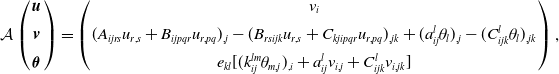 \begin{align*} \mathcal{A}\left (\begin{array}{c}{\boldsymbol{u}}\\[5pt] {\boldsymbol{v}}\\[5pt] {\boldsymbol{\theta }} \end{array}\right )= \left (\begin{array}{c} v_i\\[5pt] (A_{ijrs}u_{r,s}+B_{ijpqr}u_{r,pq})_{,j}-(B_{rsijk}u_{r,s}+C_{kjipqr}u_{r,pq})_{,jk} +(a_{ij}^l\theta _l)_{,j}-(C_{ijk}^l\theta _l)_{,jk}\\[5pt] e_{kl}[(k_{ij}^{lm}\theta _{m,j})_{,i}+a_{ij}^lv_{i,j}+C_{ijk}^lv_{i,jk}] \end{array}\right ), \end{align*}
where
 $e_{kl}$
is the inverse of the matrix
$e_{kl}$
is the inverse of the matrix
 $d_{lj}$
.
$d_{lj}$
.
We remark that the domain of the operator
 $\mathcal{A}$
is the subspace made by elements
$\mathcal{A}$
is the subspace made by elements
 $({\boldsymbol{u}},{\boldsymbol{v}},{\boldsymbol{\theta }})$
such that
$({\boldsymbol{u}},{\boldsymbol{v}},{\boldsymbol{\theta }})$
such that
 ${\boldsymbol{v}}\in{\boldsymbol{W}}_0^{2,2}(B)$
,
${\boldsymbol{v}}\in{\boldsymbol{W}}_0^{2,2}(B)$
,
 $(k_{ij}^{lm}\theta _{,j})_{,i}\in{\boldsymbol{L}}^2(B)$
and
$(k_{ij}^{lm}\theta _{,j})_{,i}\in{\boldsymbol{L}}^2(B)$
and
 $(A_{ijrs}u_{r,s}+B_{ijpqr}u_{r,pq})_{,j}-(B_{rsijk}u_{r,s}+C_{kjipqr}u_{r,pq})_{,jk} +(a_{ij}^l\theta _l)_{,j}-(C_{ijk}^l\theta _l)_{,jk}\in{\boldsymbol{L}}^2(B)$
. Obviously, it is a dense subspace in
$(A_{ijrs}u_{r,s}+B_{ijpqr}u_{r,pq})_{,j}-(B_{rsijk}u_{r,s}+C_{kjipqr}u_{r,pq})_{,jk} +(a_{ij}^l\theta _l)_{,j}-(C_{ijk}^l\theta _l)_{,jk}\in{\boldsymbol{L}}^2(B)$
. Obviously, it is a dense subspace in
 $\mathcal{H}$
.
$\mathcal{H}$
.
It is relevant noting that we can write our problem in the form:
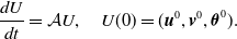 \begin{equation} \frac{dU}{dt}=\mathcal{A}U,\quad U(0)=({\boldsymbol{u}}^0,{\boldsymbol{v}}^0,{\boldsymbol{\theta }}^0). \end{equation}
This is the Cauchy problem which is defined in the space
 $\mathcal{H}$
that we will study in the next sections.
$\mathcal{H}$
that we will study in the next sections.
3. Well-posedness
In this section, we will prove that the operator
 $\mathcal{A}$
generates a contractive semigroup of linear operators. Therefore, the existence, uniqueness and the continuous dependence with respect to the initial conditions will be concluded.Footnote
2
$\mathcal{A}$
generates a contractive semigroup of linear operators. Therefore, the existence, uniqueness and the continuous dependence with respect to the initial conditions will be concluded.Footnote
2
Lemma 1.
For every
 $U=({\boldsymbol{u}},{\boldsymbol{v}},{\boldsymbol{\theta }})\in \mathrm{Dom}(\mathcal{A})$
, the following inequality
$U=({\boldsymbol{u}},{\boldsymbol{v}},{\boldsymbol{\theta }})\in \mathrm{Dom}(\mathcal{A})$
, the following inequality
 \begin{equation*}Re\langle \mathcal {A}U,U\rangle \leqslant 0\end{equation*}
holds.
Proof. If we apply the definition of the operator and we use boundary conditions (2.3), after the use of the divergence theorem we obtain that
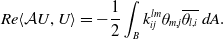 \begin{equation*}Re\langle \mathcal {A}U,U\rangle =-\frac {1}{2}\int _B k_{ij}^{lm}\theta _{m,j}\overline {\theta _{l,i}}\, dA.\end{equation*}
In view of the assumptions (iii)–(iv), we see that the lemma is proved.
Lemma 2.
The resolvent of the operator
 $\mathcal{A}$
contains the origin.
$\mathcal{A}$
contains the origin.
Proof. Let us consider
 $({\boldsymbol{f}}_1,{\boldsymbol{f}}_2,{\boldsymbol{f}}_3)\in \mathcal{H}$
. We need to solve the system:
$({\boldsymbol{f}}_1,{\boldsymbol{f}}_2,{\boldsymbol{f}}_3)\in \mathcal{H}$
. We need to solve the system:
 \begin{align*} \mathcal{A}\left (\begin{array}{c}{\boldsymbol{u}}\\[5pt] {\boldsymbol{v}}\\[5pt] {\boldsymbol{\theta }} \end{array}\right )= \left (\begin{array}{c}{\boldsymbol{f}}_1\\[5pt] {\boldsymbol{f}}_2\\[5pt] {\boldsymbol{f}}_3 \end{array}\right ). \end{align*}
That is, we find that
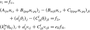 \begin{equation} \begin{array}{l} v_i=f_{1i},\\[5pt] (A_{ijrs}u_{r,s}+B_{ijpqr}u_{r,pq})_{,j} -(B_{rsijk}u_{r,s}+C_{kjipqr}u_{r,pq})_{,jk}\\[5pt] \qquad +\;(a_{ij}^l\theta _{,l})_{,j}-(C_{ijk}^l\theta _l)_{,jk}=f_{2i},\\[5pt] (k_{ij}^{lm}\theta _{m,j})_{,i}+a_{ij}^lv_{i,j}+C_{ijk}^lv_{i,jk}=e_{kl}f_{3k}. \end{array} \end{equation}
We can obtain
 $\boldsymbol{v}$
from the first equation. Then, we find that
$\boldsymbol{v}$
from the first equation. Then, we find that
 \begin{equation*}(k_{ij}^{lm}\theta _{m,j})_{,i}=e_{kl}f_{3k}-a_{ij}^l\,f_{1i,j}-C_{ijk}^l\,f_{1i,jk}.\end{equation*}
It is clear that we can solve this system assuming null Dirichlet boundary conditions. In fact, the solution satisfies the conditions for the third component of the domain of the operator. If we substitute
 $\boldsymbol{\theta }$
into the second component of the system (3.1), we can get the solution after the use of the Lax-Milgram lemma (see [Reference Ieşan13]). Indeed, we can prove that
$\boldsymbol{\theta }$
into the second component of the system (3.1), we can get the solution after the use of the Lax-Milgram lemma (see [Reference Ieşan13]). Indeed, we can prove that
 \begin{equation*}\|({\boldsymbol{u}},{\boldsymbol{v}},{\boldsymbol {\theta }})\|\leqslant K \|({\boldsymbol{f}}_1,{\boldsymbol{f}}_2,{\boldsymbol{f}}_3)\|,\end{equation*}
where
 $K$
is independent of the solution.
$K$
is independent of the solution.
Since the domain of the operator is dense, we can apply the Lumer-Phillips corollary to the Hille-Yosida theorem to prove the following.
Theorem 3.1.
The operator
 $\mathcal{A}$
generates a contractive semigroup on the Hilbert space
$\mathcal{A}$
generates a contractive semigroup on the Hilbert space
 $\mathcal{H}$
.
$\mathcal{H}$
.
In view of this theorem, we can conclude that our problem is well-posed in the sense of Hadamard.
4. Exponential stability
The aim of this section is to provide a sufficient condition on the coupling terms to guarantee the exponential stability of the solutions to our problem.
We start by considering the operator
 \begin{equation*}P_l({\boldsymbol{u}})=a_{ij}^lu_{i,j}+C_{ijk}^lu_{i,jk}\quad \hbox {for}\quad l=1,2.\end{equation*}
From now on, we will assume that
-
(v) The operator
${\boldsymbol{P}}=(P_1,P_2)$
is elliptic in
$B$
.


It is relevant to note that, in view of the boundary conditions (2.3), we can conclude that (see [Reference Liu and Zheng17, p. 14])
 \begin{equation} \|{\boldsymbol{u}}\|_{{\boldsymbol{W}}^{2,2}(B)}\leqslant C\|{\boldsymbol{P}}({\boldsymbol{u}})\|_{{\boldsymbol{L}}^2(B)}, \end{equation}
where
 $C$
is a positive constant which is independent of
$C$
is a positive constant which is independent of
 $\boldsymbol{u}$
.
$\boldsymbol{u}$
.
With the proposed assumption, and thanks to estimate (4.1), we can obtain the following result.
Theorem 4.1.
Let us assume that the operator
 $\boldsymbol{P}$
satisfies condition (v). Then, there exist two positive constants
$\boldsymbol{P}$
satisfies condition (v). Then, there exist two positive constants
 $M$
and
$M$
and
 $\omega$
such that
$\omega$
such that
 \begin{equation*}\|U(t)\|\leqslant M e^{-\omega t}\|U(0)\|\end{equation*}
for every
 $U(0)$
in the domain of the operator
$U(0)$
in the domain of the operator
 $\mathcal{A}$
.
$\mathcal{A}$
.
The proof of this theorem is based in the following lemmas.
Lemma 3.
The imaginary axis is included at the resolvent of the operator
 $\mathcal{A}$
.
$\mathcal{A}$
.
Proof. In order to prove this lemma, we start by following the arguments used in the book of Liu and Zheng [Reference Liu and Zheng17, p. 25]. There, the proof uses a contradiction procedure. It is assumed that the thesis of the lemma does not hold and then, in view of a series of comments, and that zero belongs to the resolvent of
 $\mathcal{A}$
, we can find (see, again, [Reference Liu and Zheng17, p. 25]) a sequence of real numbers
$\mathcal{A}$
, we can find (see, again, [Reference Liu and Zheng17, p. 25]) a sequence of real numbers
 $\beta _n\in \mathbb{R}$
, with
$\beta _n\in \mathbb{R}$
, with
 $\beta _n\rightarrow \beta \neq 0$
, and a sequence of elements
$\beta _n\rightarrow \beta \neq 0$
, and a sequence of elements
 $U_n=({\boldsymbol{u}}_n,{\boldsymbol{v}}_n,{\boldsymbol{\theta }}_n)$
in the domain of the operator, with unit norm, such that
$U_n=({\boldsymbol{u}}_n,{\boldsymbol{v}}_n,{\boldsymbol{\theta }}_n)$
in the domain of the operator, with unit norm, such that
 \begin{equation} \|(i\beta _n I-\mathcal{A})U_n\|_{\mathcal{H}}\rightarrow 0\quad \hbox{as}\quad n\rightarrow \infty. \end{equation}
This condition is equivalent to assume that
 \begin{align} i\beta u_i-v_i\rightarrow 0 \quad \hbox{in}\quad W^{2,2}_0(B), \end{align}
 \begin{align} &i\beta v_i-\Big ((A_{ijrs}u_{r,s}+B_{ijpqr}u_{r,pq})_{,j}-(B_{rsijk}u_{r,s}+C_{kjipqr}u_{r,pq})_{,jk}\nonumber \\[5pt] &\quad +(a_{ij}^l\theta _{,l})_{,j}-(C_{ijk}^l\theta _l)_{,jk}\Big ) \rightarrow 0 \quad \hbox{in}\quad L^2(B), \end{align}
 \begin{align} i\beta d_{lk}\theta _k-\Big ((k_{ij}^{lm}\theta _{m,j})_{,i}+a_{ij}^lv_{i,j}+C_{ijk}^lv_{i,jk}\Big ) \rightarrow 0 \quad \hbox{in}\quad L^2(B). \end{align}
We note that we have omitted the sub-index
 $n$
in convergences (4.3)–(4.5) for the sake of simplicity in the notation.
$n$
in convergences (4.3)–(4.5) for the sake of simplicity in the notation.
Now, from the dissipation inequality and the assumption on the thermal variables, we have that
 \begin{equation*}{\boldsymbol {\theta }}\rightarrow {\textbf{0}} \quad \hbox {in}\quad {\boldsymbol{W}}^{1,2}(B).\end{equation*}
If we multiply convergence (4.5) by
 $\displaystyle \frac{1}{\beta }{\boldsymbol{P}}({\boldsymbol{u}})$
, we find that
$\displaystyle \frac{1}{\beta }{\boldsymbol{P}}({\boldsymbol{u}})$
, we find that
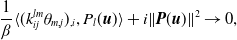 \begin{equation*}\frac {1}{\beta } \langle (k_{ij}^{lm}\theta _{m,j})_{,i}, P_l({\boldsymbol{u}})\rangle +i\|{\boldsymbol{P}}({\boldsymbol{u}})\|^2\rightarrow 0,\end{equation*}
and we can apply the divergence theorem to obtain that
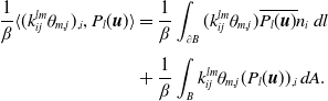 \begin{align} \frac{1}{\beta } \langle (k_{ij}^{lm}\theta _{m,j})_{,i}, P_l({\boldsymbol{u}})\rangle & = \frac{1}{\beta }\int _{\partial B} (k_{ij}^{lm}\theta _{m,j}) \overline{P_l({\boldsymbol{u}})}n_i\, dl \nonumber \\[5pt] & +\frac{1}{\beta }\int _B k_{ij}^{lm}\theta _{m,j} (P_l({\boldsymbol{u}}))_{,i}\,dA. \end{align}
where
 $n_i$
is the normal vector to
$n_i$
is the normal vector to
 $\partial B$
.
$\partial B$
.
We note that
 $\frac{1}{\beta }({\boldsymbol{P}}({\boldsymbol{u}}))_{,i}$
is bounded in view of convergences (4.4) and (4.5) and the fact that the operator defining the elastic part is elliptic. Therefore, the last integral in (4.6) vanishes since
$\frac{1}{\beta }({\boldsymbol{P}}({\boldsymbol{u}}))_{,i}$
is bounded in view of convergences (4.4) and (4.5) and the fact that the operator defining the elastic part is elliptic. Therefore, the last integral in (4.6) vanishes since
 ${\boldsymbol{\theta }}\rightarrow{\textbf{0}}$
in
${\boldsymbol{\theta }}\rightarrow{\textbf{0}}$
in
 ${\boldsymbol{W}}^{1,2}(B)$
. To show that the first integral tends to zero, we note that we can apply the following estimates
${\boldsymbol{W}}^{1,2}(B)$
. To show that the first integral tends to zero, we note that we can apply the following estimates
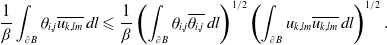 \begin{equation*}\frac {1}{\beta }\int _{\partial B} \theta _{i,j}\overline {u_{k,lm}}\, dl\leqslant \frac {1}{\beta }\left (\int _{\partial B}\theta _{i,j}\overline {\theta _{i,j}}\,dl\right )^{1/2} \left (\int _{\partial B}u_{k,lm}\overline {u_{k,lm}}\,dl\right )^{1/2}.\end{equation*}
But we also have
 \begin{equation*}\frac {1}{\beta ^{1/2}}\left (\int _{\partial B}\theta _{i,j}\overline {\theta _{i,j}}\,dl\right )^{1/2} \leqslant C_1 \left (\int _{B}\nabla \theta _{i}\overline {\nabla \theta _{i}}\,dA\right )^{1/4} \frac {1}{\beta ^{1/2}}\left (\int _{B}\Delta \theta _{i}\overline {\Delta \theta _{i}}\,dA\right )^{1/4}\end{equation*}
since
 $\theta _i$
vanishes at the boundary. At the same time, we find that
$\theta _i$
vanishes at the boundary. At the same time, we find that
 \begin{equation*}\frac {1}{\beta ^{1/2}} \left (\int _{\partial B}u_{k,lm}\overline {u_{k,lm}}\,dl\right )^{1/2}\leqslant C_2 \left (\int _B \Delta u_k \overline {\Delta u_k}\, dA\right )^{1/4} \frac {1}{\beta ^{1/2}} \left (\int _B \Delta ^2 u_k\overline {\Delta ^2 u_k}\, dA\right )^{1/4}\end{equation*}
whenever
 $u_i$
and
$u_i$
and
 $\nabla u_i$
vanish at the boundary. The parameters
$\nabla u_i$
vanish at the boundary. The parameters
 $C_1$
and
$C_1$
and
 $C_2$
are independent of the functions.
$C_2$
are independent of the functions.
But we note that
 $\displaystyle \beta ^{-1}\Big (\int _B\Delta \theta _i\overline{\Delta \theta _i}\, dA\Big )^{1/2}$
and
$\displaystyle \beta ^{-1}\Big (\int _B\Delta \theta _i\overline{\Delta \theta _i}\, dA\Big )^{1/2}$
and
 $\displaystyle \beta ^{-1}\Big (\int _B\Delta ^2 u_k \overline{\Delta ^2 u_k}\, dA\Big )^{1/2}$
are boundedFootnote
3
as well as
$\displaystyle \beta ^{-1}\Big (\int _B\Delta ^2 u_k \overline{\Delta ^2 u_k}\, dA\Big )^{1/2}$
are boundedFootnote
3
as well as
 $\displaystyle \int _B \Delta u_k\Delta u_k \, dA$
. Since
$\displaystyle \int _B \Delta u_k\Delta u_k \, dA$
. Since
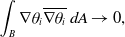 \begin{equation*}\int _B \nabla \theta _{i}\overline {\nabla \theta _{i}}\, dA\rightarrow 0,\end{equation*}
we can conclude that the first integral in (4.6) also tends to zero, and therefore, it follows that
 $\|{\boldsymbol{P}}({\boldsymbol{u}})\|\rightarrow 0$
. But, as we can see the estimate (4.1) we also conclude that
$\|{\boldsymbol{P}}({\boldsymbol{u}})\|\rightarrow 0$
. But, as we can see the estimate (4.1) we also conclude that
 ${\boldsymbol{u}}\rightarrow{\textbf{0}}$
in
${\boldsymbol{u}}\rightarrow{\textbf{0}}$
in
 ${\boldsymbol{W}}^{2,2}(B)$
. Now, an easy argument also shows that
${\boldsymbol{W}}^{2,2}(B)$
. Now, an easy argument also shows that
 ${\boldsymbol{v}}\rightarrow{\textbf{0}}$
in
${\boldsymbol{v}}\rightarrow{\textbf{0}}$
in
 ${\boldsymbol{L}}^2(B)$
and we arrive to a contradiction. It comes from the fact that we assume that there would exist an element of the imaginary axis at the spectrum. Therefore, the lemma is proved.
${\boldsymbol{L}}^2(B)$
and we arrive to a contradiction. It comes from the fact that we assume that there would exist an element of the imaginary axis at the spectrum. Therefore, the lemma is proved.
Lemma 4. The asymptotic condition
 \begin{equation*}\overline {\lim _{|\beta |\rightarrow \infty }} \|(i\beta I-\mathcal {A})^{-1}\| \lt \infty \end{equation*}
holds.
Proof. The proof follows a similar strategy to the one used in the proof of the previous lemma. Let us assume that the above asymptotic condition does not hold. Therefore, there will exist a sequence of real numbers
 $\beta _n\rightarrow \infty$
and a sequence of unit norm vectors
$\beta _n\rightarrow \infty$
and a sequence of unit norm vectors
 $U_n$
, at the domain of the operator
$U_n$
, at the domain of the operator
 $\mathcal{A}$
, such that convergence (4.2) is satisfied. In view of the fact that the arguments used in the proof of the previous lemma hold whenever
$\mathcal{A}$
, such that convergence (4.2) is satisfied. In view of the fact that the arguments used in the proof of the previous lemma hold whenever
 $\beta _n$
does not tend to zero, we can conclude the thesis of this lemma.
$\beta _n$
does not tend to zero, we can conclude the thesis of this lemma.
We have proved the exponential decay result for the solutions to our problem. It is worth saying that an easy example (for a given operator
 $\boldsymbol{P}$
to be elliptic) corresponds to assume
$\boldsymbol{P}$
to be elliptic) corresponds to assume
 \begin{equation*}C_{1,ij}^1 u_{1,ij}=\Delta u_1,\quad C_{2,ij}^2u_{2,ij}=\Delta u_2,\end{equation*}
meanwhile the remaining coefficients
 $\beta _{ij}^l$
and
$\beta _{ij}^l$
and
 $C_{ijk}^l$
vanish.
$C_{ijk}^l$
vanish.
5. Analyticity of the semigroup
The aim of this section is to prove the analyticity of the solutions to problem (2.7) whenever the conditions (i)–(v) hold. As a consequence, we will obtain the uniqueness of the backward in time problem, and so, it will be proved that the unique solution vanishing for every time, after a certain value, is the null solution.
Theorem 5.1.
The semigroup generated by the operator
 $\mathcal{A}$
is analytic.
$\mathcal{A}$
is analytic.
Proof. Since we have shown that the imaginary axis is contained at the resolvent of the operator, the theorem will be concluded if we see that
 \begin{equation} \overline{\lim _{|\beta |\rightarrow \infty }}\|\beta ^{-1}(i\beta I-\mathcal{A})^{-1}\|\lt \infty. \end{equation}
We will prove condition (5.1) by contradiction. Let us assume the existence of a sequence
 $\beta _n\rightarrow \infty$
and a sequence of unit norm vectors
$\beta _n\rightarrow \infty$
and a sequence of unit norm vectors
 $U_n$
(at the domain of the operator) such that
$U_n$
(at the domain of the operator) such that
 \begin{equation} i U_n-\beta _n^{-1}\mathcal{A}U_n\rightarrow 0\quad \hbox{in}\quad \mathcal{H}, \end{equation}
and we will conclude that
 $U_n\rightarrow 0$
, which is a contradiction. We note that condition (5.2) is equivalent to the convergences:
$U_n\rightarrow 0$
, which is a contradiction. We note that condition (5.2) is equivalent to the convergences:
 \begin{align} i u_i-\beta ^{-1}v_i \rightarrow 0 \quad \hbox{in}\quad W^{2,2}(B), \end{align}
 \begin{align} & i v_i-\beta ^{-1}\Big ((A_{ijrs}u_{r,s}+B_{ijpqr}u_{r,pq})_{,j}-(B_{rsijk}u_{r,s}+C_{kjipqr}u_{r,pq})_{,jk}\nonumber \\[5pt] &\qquad +(a_{ij}^l\theta _{,l})_{,j}-(C_{ijk}^l\theta _l)_{,jk}\Big ) \rightarrow 0 \quad \hbox{in}\quad L^{2}(B), \end{align}
 \begin{align} i d_{lk}\theta _k-\beta ^{-1}\Big ((k_{ij}^{lm}\theta _{m,j})_{,i}+a_{ij}^lv_{i,j}+C_{ijk}^lv_{i,jk}\Big ) \rightarrow 0 \quad \hbox{in}\quad L^{2}(B), \end{align}
where we omit again the sub-index ‘
 $n$
’ to simplify the notation.
$n$
’ to simplify the notation.
If we multiply convergence (5.2) by
 $U_n$
, we obtain that
$U_n$
, we obtain that
 \begin{equation} \beta ^{-1/2}{\boldsymbol{\theta }} \rightarrow{\textbf{0}}\quad \hbox{in}\quad{\boldsymbol{W}}^{1,2}(B). \end{equation}
Gagliardo-Niremberg’s inequality implies that
 \begin{equation*}\|\beta ^{-1/2}{\boldsymbol{v}}\|_{{\boldsymbol{W}}^{1,2}(B)}^2\leqslant C \beta ^{-1}\|{\boldsymbol{v}}\|_{{\boldsymbol{W}}^{2,2}(B)}\|{\boldsymbol{v}}\|_{{\boldsymbol{L}}^2(B)}.\end{equation*}
As
 $\beta ^{-1}\|{\boldsymbol{v}}\|_{{\boldsymbol{W}}^{2,2}(B)}$
and
$\beta ^{-1}\|{\boldsymbol{v}}\|_{{\boldsymbol{W}}^{2,2}(B)}$
and
 $\|{\boldsymbol{v}}\|_{{\boldsymbol{L}}^2(B)}$
are bounded, we see that
$\|{\boldsymbol{v}}\|_{{\boldsymbol{L}}^2(B)}$
are bounded, we see that
 $\|\beta ^{-1/2}{\boldsymbol{v}}\|_{{\boldsymbol{W}}^{1,2}(B)}$
is bounded.
$\|\beta ^{-1/2}{\boldsymbol{v}}\|_{{\boldsymbol{W}}^{1,2}(B)}$
is bounded.
If we multiply convergence (5.5) by
 $\boldsymbol{\theta }$
, we get
$\boldsymbol{\theta }$
, we get
 \begin{equation*}i\langle d_{kl}\theta _k,\theta _l\rangle +\langle \beta ^{-1/2} C_{ijk}^lv_{i,j},\beta ^{-1/2}\theta _{l,k}\rangle \rightarrow 0.\end{equation*}
In view of convergence (5.6) and that
 $\|\beta ^{-1/2}{\boldsymbol{v}}\|_{{\boldsymbol{W}}^{1/2}(B)}$
is bounded, we conclude that
$\|\beta ^{-1/2}{\boldsymbol{v}}\|_{{\boldsymbol{W}}^{1/2}(B)}$
is bounded, we conclude that
 \begin{equation*}{\boldsymbol {\theta }}\rightarrow {\textbf{0}} \quad \hbox {in}\quad {\boldsymbol{L}}^2(B).\end{equation*}
It follows that
 \begin{equation*}i{\boldsymbol{P}}({\boldsymbol{u}})+\beta ^{-1}(k_{ij}^{lm}\theta _{m,j})_{,i}\rightarrow 0 \quad \hbox {in} \quad {\boldsymbol{L}}^2(B).\end{equation*}
Since
 $\boldsymbol{u}$
is bounded in
$\boldsymbol{u}$
is bounded in
 ${\boldsymbol{W}}^{2,2}(B)$
and, in view of condition (iii), we see that
${\boldsymbol{W}}^{2,2}(B)$
and, in view of condition (iii), we see that
 \begin{equation*}\|\beta ^{-1} {\boldsymbol {\theta }}\|_{{\boldsymbol{W}}^{2,2}(B)}\lt \infty .\end{equation*}
From convergence (5.4) and condition (iv) we have
 \begin{equation*}\|\beta ^{-1} {\boldsymbol{u}}\|_{{\boldsymbol{W}}^{4,2}(B)}\lt \infty .\end{equation*}
We use again the Gagliardo-Niremberg’s inequality to see
 \begin{equation*}\|\beta ^{-1/2}{\boldsymbol{u}}\|^2_{{\boldsymbol{W}}^{3,2}(B)}\leqslant C\beta ^{-1}\|{\boldsymbol{u}}\|_{{\boldsymbol{W}}^{4,2}(B)}\|{\boldsymbol{u}}\|_{{\boldsymbol{W}}^{2,2}(B)}.\end{equation*}
In the next step, we multiply convergence (5.5) by
 ${\boldsymbol{P}}({\boldsymbol{u}})$
to find that
${\boldsymbol{P}}({\boldsymbol{u}})$
to find that
 \begin{equation} i\|{\boldsymbol{P}}({\boldsymbol{u}})\|^2-\langle \beta ^{-1/2}k_{ij}^{lm}\theta _{m,j},\beta ^{-1/2}(P_l({\boldsymbol{u}}))_{,i}\rangle +\beta ^{-1} \int _{\partial B}k_{ij}^{lm}\theta _{m,j}\overline{P_l({\boldsymbol{u}})}n_i\, dl\rightarrow 0. \end{equation}
Now, we want to see that this last integral tends to zero. We note that
 \begin{equation*}\beta ^{-1} \int _{\partial B}k_{ij}^{lm}\theta _{m,j}\overline {P_l({\boldsymbol{u}})}n_i\, dl \leqslant C\beta ^{-3/4}\|\nabla {\boldsymbol {\theta }}\|_{{\boldsymbol{L}}^2(\partial B)}\beta ^{-1/4}\|\Delta {\boldsymbol{u}}\|_{{\boldsymbol{L}}^2(\partial B)}.\end{equation*}
But we have
 \begin{align} \displaystyle \beta ^{-3/4}\|\nabla{\boldsymbol{\theta }}\|_{{\boldsymbol{L}}^2(\partial B)} \leqslant C\left ( \beta ^{-1}\|{\boldsymbol{\theta }}\|_{{\boldsymbol{W}}^{2,2}(B)}\right )^{1/2} \left ( \beta ^{-1/2}\|{\boldsymbol{\theta }}\|_{{\boldsymbol{W}}^{1,2}(B)}\right )^{1/2}, \end{align}
 \begin{align} \beta ^{-1/4}\|\Delta{\boldsymbol{u}}\|_{{\boldsymbol{L}}^2(\partial B)} \leqslant C\left ( \beta ^{-1/2}\|\Delta{\boldsymbol{u}}\|_{{\boldsymbol{W}}^{1,2}(B)}\right )^{1/2} \|\Delta{\boldsymbol{u}}\|_{{\boldsymbol{L}}^2(B)}^{1/2}. \end{align}
We note that the right hand-side of (5.9) is bounded and the right hand-side of (5.8) tends to zero. Then, we obtain that the last integral of convergence (5.7) converges to zero. We also note that the inner product in (5.8) tends to zero thanks to convergence (5.6) and the fact that
 $\beta ^{-1}\|{\boldsymbol{u}}\|_{{\boldsymbol{W}}^{4,2}(B)}$
is bounded. Thus, we see that
$\beta ^{-1}\|{\boldsymbol{u}}\|_{{\boldsymbol{W}}^{4,2}(B)}$
is bounded. Thus, we see that
 \begin{equation*}{\boldsymbol{u}}\rightarrow {\textbf{0}} \quad \hbox {in}\quad {\boldsymbol{W}}^{2,2}(B).\end{equation*}
If we multiply convergence (5.4) by
 $\boldsymbol{v}$
, we also obtain
$\boldsymbol{v}$
, we also obtain
 \begin{equation*}{\boldsymbol{v}}\rightarrow {\textbf{0}}\quad \hbox {in}\quad {\boldsymbol{L}}^2(B).\end{equation*}
We have arrived to a contradiction because we assumed that
 $\|U_n\|=1$
, and so, the theorem is proved.
$\|U_n\|=1$
, and so, the theorem is proved.
In view of the fact that the semigroup generated by operator
 $\mathcal{A}$
is analytic, we can conclude the following.
$\mathcal{A}$
is analytic, we can conclude the following.
Corollary 1.
Let us assume that the solution
 $U(t)$
to problem (2.7) vanishes for every
$U(t)$
to problem (2.7) vanishes for every
 $t\geqslant t_0\geqslant 0$
. Then,
$t\geqslant t_0\geqslant 0$
. Then,
 $U(t)\equiv 0$
.
$U(t)\equiv 0$
.
6. Hyperbolic case
In this section, we sketch how to extend the exponential stability of the solutions to the case of the Green-Lindsay dissipation mechanisms (see [Reference Green and Lindsay10] for further details regarding this theory).
In this case, the system of equations is (see [Reference Ieşan and Quintanilla11]):
 \begin{equation} \begin{array}{l} \rho \ddot{u}_i=\Big (A_{ijrs} u_{r,s}+B_{ijpqr}u_{r,pq}+a_{ij}^l(\theta _l+\alpha \dot{\theta }_l)\Big )_{,j}\\[5pt] \qquad \qquad -\Big ( B_{rsijk}u_{r,s}+C_{kjipqr}u_{r,pq}+C_{ijk}^l(\theta _l+\alpha \dot{\theta }_l)\Big )_{,jk},\\[5pt] m_{lp}\ddot{\theta }_p+d_{lp}\dot{\theta }_p=(k_{ij}^{lm}\theta _{m,j})_{,i}+a_{ij}^l\dot{{u}}_{i,j}+C_{ijk}^l\dot{{u}}_{i,jk} +b^{jl}_i\dot{\theta }_{j,i}+(b_{i}^{jl}\dot{\theta }_j)_{,i}. \end{array} \end{equation}
We note that, in this system,
 $\rho$
,
$\rho$
,
 $u_i$
,
$u_i$
,
 $A_{ijrs}$
,
$A_{ijrs}$
,
 $B_{ijpqr}$
,
$B_{ijpqr}$
,
 $C_{ijkpqr}$
,
$C_{ijkpqr}$
,
 $a_{ij}^l$
,
$a_{ij}^l$
,
 $C_{ijk}^l$
,
$C_{ijk}^l$
,
 $d_{lp}$
,
$d_{lp}$
,
 $k_{ij}^{lm}$
and
$k_{ij}^{lm}$
and
 $\theta _l$
were defined in the previous sections. However, we have now introduced several new elements. Here,
$\theta _l$
were defined in the previous sections. However, we have now introduced several new elements. Here,
 $\alpha$
is a positive constant which is considered as a relaxation parameter. We also have a new symmetric matrix
$\alpha$
is a positive constant which is considered as a relaxation parameter. We also have a new symmetric matrix
 $m_{lp}$
which is assumed to satisfy that
$m_{lp}$
which is assumed to satisfy that
 \begin{equation*}\alpha d_{ij}-m_{ij}\quad \hbox {and}\quad m_{ij}\end{equation*}
are positive definite matrices. Another new component is the matrix
 $b_i^{jl}$
which is assumed to satisfy the following symmetry:
$b_i^{jl}$
which is assumed to satisfy the following symmetry:
 \begin{equation*}b_i^{jl}=b_i^{lj}.\end{equation*}
It is also worth to note that we need to modify assumption (iii), which is now replaced by the following one:
-
(iii*) There exists a positive constant
$D$
such that
\begin{equation*}k_{ij}^{lm}\theta _{l,i}\theta _{m,j}+2 b_i^{jl}\dot {\theta }_j\theta _{l,i}+(d_{ij}\alpha -m_{ij})\dot {\theta }_i\dot {\theta }_j \geqslant D(\theta _{i,j}\theta _{i,j}+\dot {\theta }_i\dot {\theta }_i).\end{equation*}


In this case, we also need to impose the initial conditions (2.2) and
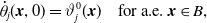 \begin{equation} \dot{\theta }_j({\boldsymbol{x}},0)=\vartheta _j^0({\boldsymbol{x}})\quad \hbox{for a.e. }{\boldsymbol{x}}\in B, \end{equation}
and boundary conditions (2.3).
We can consider the problem defined by the system (6.1), the initial conditions (2.2) and (6.2), and the boundary conditions (2.3).
This problem can be written in the abstract form (2.7), where
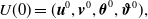 \begin{equation*}U(0)=({\boldsymbol{u}}^0,{\boldsymbol{v}}^0,{\boldsymbol {\theta }}^0,{\boldsymbol {\vartheta }}^0),\end{equation*}
and
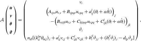 \begin{align*} \mathcal{A}\left (\begin{array}{c}{\boldsymbol{u}}\\[5pt] {\boldsymbol{v}}\\[5pt] {\boldsymbol{\theta }}\\[5pt] {\boldsymbol{\vartheta }} \end{array}\right )= \left (\begin{array}{c} v_i\\[5pt] \Big (A_{ijrs} u_{r,s}+B_{ijpqr}u_{r,pq}+a_{ij}^l(\theta _l+\alpha \dot{\theta }_l)\Big )_{,j}\\[5pt] \qquad \qquad -\Big ( B_{rsijk}u_{r,s}+C_{kjipqr}u_{r,pq}+C_{ijk}^l(\theta _l+\alpha \dot{\theta }_l)\Big )_{,jk}\\[5pt] \vartheta _i\\[5pt] n_{dl}[(k_{ij}^{lm}\theta _{m,j})_{,i}+a_{ij}^lv_{i,j}+C_{ijk}^lv_{i,jk}+b_i^{jl}\vartheta _{j,i}+(b_i^{jl}\vartheta _j)_{,i} -d_{lp}\vartheta _p] \end{array}\right ), \end{align*}
where
 $n_{dl}$
is the inverse of the matrix
$n_{dl}$
is the inverse of the matrix
 $m_{lp}$
.
$m_{lp}$
.
This problem is defined in the modified Hilbert space:
 \begin{equation*}\mathcal {H}={\boldsymbol{W}}^{2,2}_0(B)\times {\boldsymbol{L}}^2(B)\times {\boldsymbol{W}}_0^{1,2}(B)\times {\boldsymbol{L}}^2(B).\end{equation*}
We note that we can consider the inner product with the following square of the norm:
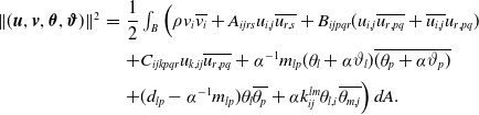 \begin{align*} \begin{array}{lll} \|({\boldsymbol{u}},{\boldsymbol{v}},{\boldsymbol{\theta }},{\boldsymbol{\vartheta }})\|^2&=&\dfrac{1}{2}\int _B \Big (\rho v_i\overline{v_i}+A_{ijrs}u_{i,j}\overline{u_{r,s}}+ B_{ijpqr}(u_{i,j}\overline{u_{r,pq}}+\overline{u_{i,j}}u_{r,pq})\\[9pt] && +C_{ijkpqr}u_{k,ij}\overline{u_{r,pq}}+\alpha ^{-1}m_{lp}(\theta _l+\alpha \vartheta _l)\overline{(\theta _p +\alpha \vartheta _p)}\\[5pt] && +(d_{lp}-\alpha ^{-1}m_{lp})\theta _l\overline{\theta _p}+ \alpha k_{ij}^{lm}\theta _{l,i}\overline{\theta _{m,j}}\Big )\,dA. \end{array} \end{align*}
This norm is equivalent to the usual one in the Hilbert space
 $\mathcal{H}$
.
$\mathcal{H}$
.
We also note that the domain of the operator
 $\mathcal{A}$
is dense and it can be obtained as the elements of the Hilbert space
$\mathcal{A}$
is dense and it can be obtained as the elements of the Hilbert space
 $\mathcal{H}$
such that
$\mathcal{H}$
such that
 \begin{align*} \begin{array}{l}{\boldsymbol{v}}\in{\boldsymbol{W}}_0^{2,2}(B),\quad{\boldsymbol{\vartheta }}\in{\boldsymbol{W}}_0^{1,2}(B),\\[5pt] (B_{ijpqr}u_{r,pq})_{,j}+(B_{rsijk}u_{r,s}+C_{ijkpqr}u_{r,pq}+C_{ijk}^l(\theta _l+\alpha \vartheta _l))_{,jk}\in{\boldsymbol{L}}^2(B),\\[5pt] (k_{ij}^{lm}\theta _{m,j})_{,i}\in{\boldsymbol{L}}^2(B). \end{array} \end{align*}
We note that, if
 $U=({\boldsymbol{u}},{\boldsymbol{v}},{\boldsymbol{\theta }},{\boldsymbol{\vartheta }})$
belongs to the domain of the operator
$U=({\boldsymbol{u}},{\boldsymbol{v}},{\boldsymbol{\theta }},{\boldsymbol{\vartheta }})$
belongs to the domain of the operator
 $\mathcal{A}$
, we have
$\mathcal{A}$
, we have
 \begin{equation*}Re\langle \mathcal {A}U,U\rangle =-\frac {1}{2}\int _B \Big ( k_{ij}^{lm}\theta _{l,i}\overline {\theta _{m,j}} +b_i^{jl}(\vartheta _j\overline {\theta _{l,i}}+\overline {\vartheta _j}\theta _{l,i}) +(d_{ij}\alpha -m_{ij})\vartheta _i\overline {\vartheta _j}\Big )\, dA,\end{equation*}
which is less or equal than zero thanks to condition (iii
 $^*$
).
$^*$
).
We can also follow a similar argument to the one used previously to show that zero belongs to the resolvent of the operator. Therefore, we can obtain the same result provided in Theorem 3.1 in our case.
We could also prove that Theorem 4.1 also holds in this hyperbolic case. Following the same strategy used in the proof of Lemma 3, we arrive to a sequence
 $U_n=({\boldsymbol{u}}_n,{\boldsymbol{v}}_n,{\boldsymbol{\theta }}_n,{\boldsymbol{\vartheta }}_n)$
of unit norm vectors in the domain of the operator and a sequence
$U_n=({\boldsymbol{u}}_n,{\boldsymbol{v}}_n,{\boldsymbol{\theta }}_n,{\boldsymbol{\vartheta }}_n)$
of unit norm vectors in the domain of the operator and a sequence
 $\beta _n\rightarrow \beta$
(finite or infinite but different from zero) such that condition (4.2) holds.
$\beta _n\rightarrow \beta$
(finite or infinite but different from zero) such that condition (4.2) holds.
This is equivalent to write
 \begin{align} i\beta u_i-v_i\rightarrow 0 \quad \hbox{in}\quad W^{2,2}_0(B), \end{align}
 \begin{align} & i\beta v_i-\Big (A_{ijrs} u_{r,s}+B_{ijpqr}u_{r,pq}+a_{ij}^l(\theta _l+\alpha \dot{\theta }_l)\Big )_{,j}\nonumber \\[5pt] &\qquad -\Big ( B_{rsijk}u_{r,s}+C_{kjipqr}u_{r,pq}+C_{ijk}^l(\theta _l+\alpha \dot{\theta }_l)\Big )_{,jk} \rightarrow 0 \quad \hbox{in}\quad L^2(B), \end{align}
 \begin{align} i\beta \theta _i-\vartheta _i\rightarrow 0 \quad \hbox{in}\quad W^{1,2}_0(B), \end{align}
 \begin{align} & i\beta d_{lk}\theta _k-\Big ((k_{ij}^{lm}\theta _{m,j})_{,i}+a_{ij}^lv_{i,j}+C_{ijk}^lv_{i,jk} +b^{jl}_i\vartheta _{j,i}+(b_{i}^{jl}\vartheta _j)_{,i}\nonumber \\[5pt] &\qquad -m_{lk}\vartheta _k\Big ) \rightarrow 0 \quad \hbox{in}\quad L^2(B). \end{align}
Again, the dissipation inequality implies that
 \begin{equation*}{\boldsymbol {\theta }}\rightarrow {\textbf{0}} \quad \hbox {in} \quad {\boldsymbol{W}}_0^{1,2}(B),\quad {\boldsymbol {\vartheta }}\rightarrow {\textbf{0}} \quad \hbox {in} \quad {\boldsymbol{L}}^{2}(B).\end{equation*}
The remaining part of the proof follows the same points as in the proof of Lemma 3. Therefore, we have obtained the following.
Theorem 6.1.
The problem proposed by system (6.1) with the initial conditions (2.2) and (6.2), and the boundary conditions (2.3) admits a unique solution. Furthermore, if
 $U(0)=({\boldsymbol{u}}^0,{\boldsymbol{v}}^0,{\boldsymbol{\theta }}^0,{\boldsymbol{\vartheta }}^0)$
belongs to the domain of the operator
$U(0)=({\boldsymbol{u}}^0,{\boldsymbol{v}}^0,{\boldsymbol{\theta }}^0,{\boldsymbol{\vartheta }}^0)$
belongs to the domain of the operator
 $\mathcal{A}$
, then there exist two positive constants
$\mathcal{A}$
, then there exist two positive constants
 $M$
and
$M$
and
 $\omega$
such that
$\omega$
such that
 \begin{equation*}\|U(t)\|\leqslant Me^{-\omega t}\|U(0)\|.\end{equation*}
7. Further comments
In this paper, we have proved the analyticity and the exponential decay of the solutions to the two-dimensional strain gradient thermoelasticity, with two dissipative mechanisms, in the case that we assume that the coupling terms define an elliptic operator and the dissipation is of the type of Fourier. Exponential decay has been also obtained when the dissipative structure is defined by the Green and Lindsay theory. However, it is suitable to say that the extension of these arguments to the three-dimensional case is obvious and we have restricted to the two-dimensional one for the sake of simplicity in the notation. It is important to remark that, in order to guarantee that the coupling terms define an elliptic operator, it is needed that we consider chiral materials since the tensor
 $C_{ijk}^l$
cannot vanish. Therefore, in the case of isotropic materials our analysis cannot be applied. It is also remarkable that, in the case of the strain gradient theory, we need a number of dissipative mechanisms smaller than in the case of the usual elasticity. This is because the coupling in this case is stronger.
$C_{ijk}^l$
cannot vanish. Therefore, in the case of isotropic materials our analysis cannot be applied. It is also remarkable that, in the case of the strain gradient theory, we need a number of dissipative mechanisms smaller than in the case of the usual elasticity. This is because the coupling in this case is stronger.
One could ask if the arguments and results presented in the previous sections can be applied to other thermoelastic theories. We want to express that we have tried to extend them to the Lord-Shulmann theory but we have not been able to obtain the exponential decay in this case. In view of the mathematical similarity of our problem with the plate problem, and taking into account that we cannot prove the exponential decay for the Lord-Shulmann plate [Reference Quintanilla and Racke22] but it is possible to obtain the exponential decay for the Green-Lindsay plate [Reference Quintanilla, Racke and Ueda23], one suspects that, in the general case, we cannot expect the exponential decay for the Lord-Shulmann theory of strain gradient elasticity. However, this is an open question that we hope to address in the near future.
Acknowledgements
This paper is part of the project PID2019-105118GB-I00, funded by the Spanish Ministry of Science, Innovation and Universities and FEDER ‘A way to make Europe’.
Competing interests
The authors declare none.


 Open access