


Introduction
Biological diversity has experienced significant losses as a result of a number of factors that directly or indirectly affect species. Amphibians and reptiles are among the groups most affected (Böhm et al., Reference Böhm, Collen, Baillie, Bowles, Chanson and Cox2013; Ceballos et al., Reference Ceballos, Ehrlich, Barnosky, García, Pringle and Palmer2015). Reptiles are specifically threatened by habitat loss, degradation and fragmentation, introduction of invasive species, pollution, pathogens and climate change, resulting in global population declines (Cox & Temple, Reference Cox and Temple2009).
Global climate change plays a key role in the biodiversity crisis (Butchart et al., Reference Butchart, Walpole, Collen, van Strien, Scharlemann and Almond2010), as it causes a redistribution of biodiversity patterns (Pecl et al., Reference Pecl, Araújo, Bell, Blanchard, Bonebrake and Chen2017). Many species are predicted to shift their range, mostly towards the poles or higher altitudes (Hickling et al., Reference Hickling, Roy, Hill, Fox and Thomas2006; Chen et al., Reference Chen, Hill, Ohlemüller, Roy and Thomas2011). Species adapted to high altitude habitats are thus particularly threatened by climate change because they often have low dispersal ability, a high level of habitat specialization and fragmented distributions, all of which predict low probability of range shift (Davies et al., Reference Davies, Margules and Lawrence2004). Ectothermic animals such as reptiles are further threatened by climate change because of their sensitivity to changes in the thermal landscape and low dispersal ability (Sinervo et al., Reference Sinervo, Méndez-de-la-Cruz, Miles, Heulin, Bastiaans and Villagrán-Santa Cruz2010). Mountain-dwelling species usually escape the changing thermal landscape by shifting their distributions to higher altitudes (Haines et al., Reference Haines, Stuart-Fox, Sumner, Clemann, Chapple and Melville2017) but this is possible only if the local topography allows this (Şekercioğlu et al., Reference Şekercioğlu, Schneider, Fay and Loarie2008).
Meadow vipers (Vipera ursinii complex) are among the most threatened reptiles of Europe. The Greek meadow viper Vipera graeca, a small venomous snake endemic to the Pindos mountain range of Greece and Albania that has recently been recognized as a separate species (Mizsei et al., Reference Mizsei, Jablonski, Roussos, Dimaki, Ioannidis, Nilson and Nagy2017), is the least known meadow viper in Europe and is categorized as Endangered on the IUCN Red List (Mizsei et al., Reference Mizsei, Szabolcs, Dimaki, Roussos and Ioannidis2018). The species has only 17 known populations, inhabiting alpine–subalpine meadows above 1,600 m on isolated mountaintops (Mizsei et al., Reference Mizsei, Üveges, Vági, Szabolcs, Lengyel and Pfliegler2016). The occupied habitats are the highest and coldest in the region; as the species is adapted to cold environments it is sensitive to climate change. These alpine habitats are threatened by overgrazing and habitat degradation, which simplify vegetation structure and reduce cover against potential predators. The species is strictly insectivorous, specializing on bush crickets and grasshoppers (Mizsei et al., Reference Mizsei, Boros, Lovas-Kiss, Szepesváry, Szabolcs and Rák2019), and thus it is vulnerable to changes in its primary prey resource caused by land use. Shepherds are known to intentionally kill these snakes, which are held responsible for 1–4% of lethal bites to sheep annually in Albania (E. Mizsei, unpubl. data).
Here we identify priority areas that could facilitate the long-term persistence of V. graeca. We performed single species spatial prioritization to identify areas based on conservation value attributes of the currently suitable landscape. We aimed to identify any populations likely to disappear by the 2080s and any populations likely to be strongholds where the species could benefit from targeted management and conservation. To provide guidelines for conservation, we studied the overlap between priority areas and protected areas and explored the interrelationships of the conservation value variables to identify opportunities for potential interventions.
Methods
Approach
We used spatial prioritization, an approach rarely applied to single species (Adam-Hosking et al., Reference Adam-Hosking, McAlpine, Rhodes, Moss and Grantham2015), which is based on quantifying known threats and transforming them into variables describing conservation value based on current conditions. The process consisted of (1) delimiting the study area, (2) collecting and processing data on threats to derive conservation value variables, (3) spatial prioritization of the study area based on the conservation value variables, and (4) evaluation of overlaps with current protected areas and analysis of any interrelationships between conservation value variables (Fig. 1).

Fig. 1 Flow chart of data processing and conservation value layer construction and analysis. For abbreviations, see Methods.
Habitat suitability modelling to define the study area
We defined our study area to include all V. graeca habitats identified by a habitat suitability model (Fig. 2). The model was constructed using 351 records of V. graeca, 83% of which were taken from our previous publications (Mizsei et al., Reference Mizsei, Üveges, Vági, Szabolcs, Lengyel and Pfliegler2016, Reference Mizsei, Jablonski, Roussos, Dimaki, Ioannidis, Nilson and Nagy2017) and 17% of which were new, unpublished records. Our dataset contained all known localities of V. graeca, and also included absence data from 31 localities (55 records) predicted in an earlier habitat suitability model (Mizsei et al., Reference Mizsei, Üveges, Vági, Szabolcs, Lengyel and Pfliegler2016), and where the species has not been found despite extensive searches. To account for potential spatial biases in sampling effort among sites, we resampled the presence dataset to obtain a spatially balanced subset of 71 presence records, which represented all known populations (Fig. 2). We used BIOCLIM climate variables, which have been successfully used to model the distribution of several European reptiles, including vipers (Scali et al., Reference Scali, Mangiacotti, Sacchi and Gentilli2011; Martínez-Freiria, Reference Martínez-Freiría2015; Mizsei et al., Reference Mizsei, Üveges, Vági, Szabolcs, Lengyel and Pfliegler2016). To ensure compatibility with our previous work (Mizsei et al., Reference Mizsei, Üveges, Vági, Szabolcs, Lengyel and Pfliegler2016), we used the same set of predictors: annual mean temperature (BIO1), temperature seasonality (BIO4), annual precipitation (BIO12) and precipitation seasonality (BIO15). These variables had high predictive performance and low intercorrelations (r < 0.7). We obtained these variables for current climatic conditions (mean of 1950–2000) from the WorldClim 1.4 database at 30 arc seconds resolution (Hijmans et al., Reference Hijmans, Cameron, Parra, Jones and Jarvis2005). We generated the habitat suitability model using ensemble modelling (Thuiller et al., Reference Thuiller, Georges and Engler2012) in the BIOMOD2 package in R 3.3.0 (R Core Team, 2016). We used two linear model algorithms (Generalized Linear Models, GLM; Generalized Additive Models, GAM) and three machine learning algorithms (Artificial Neural Networks, ANN; Random Forest, RF; Maximum Entropy, MaxEnt). Default settings were used to build the models (Thuiller et al., Reference Thuiller, Georges and Engler2012). To increase model accuracy we generated 10 datasets of pseudo-absences, which included real absence data and random points at least 5 km from the presence localities (a total of 10,000 points per dataset). We ran 10 replicates with each of the five modelling algorithms for the 10 pseudo-absence datasets, which resulted in 500 habitat suitability model replicates. In each model replicate we randomly divided the presence data into training (70%) and testing subsets (30%). We used the four BIOCLIM variables as predictors. We scored all individual model replicates by the true skill statistic (TSS; Allouche et al., Reference Allouche, Tsoar and Kadmon2006), retaining only models with TSS > 0.95. This filtering resulted in 275 models, which always correctly classified the testing subset and that were used to produce ensemble projections by consensus (i.e. raster cells predicted suitable in each of the 275 models). Finally, we generated a binary suitability map using the ensemble projection of the best models and defined the resulting patches as the study area for the analysis (Fig. 2).
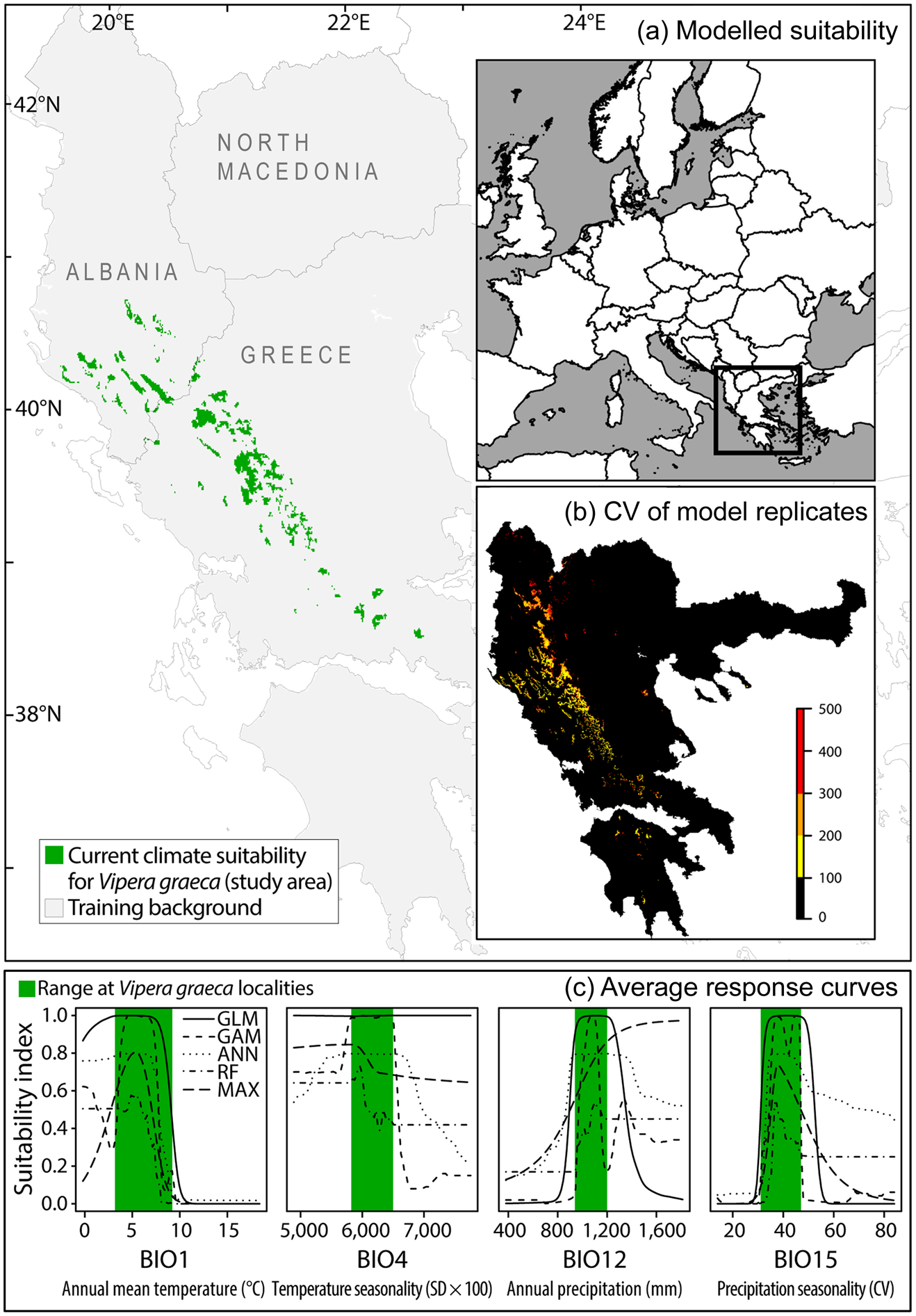
Fig. 2 (a) Area identified by the climate habitat suitability model for V. graeca in the western Balkans, (b) coefficient of variation (CV) of habitat suitability model replicates, and (c) average response curves of modelling algorithms for each predictor variable of the model, with range of values measured at V. graeca presence locations.
Variables for estimating conservation value
We used nine environmental variables of three classes to estimate the conservation value of planning units (1 ha raster cells) over the entire study area: (1) habitat suitability: climate suitability, habitat size, habitat occupancy, vegetation suitability; (2) climate change: future persistence, potential for altitudinal range shift, (3) land-use impact: habitat alteration, habitat degradation, disturbance (Fig. 1). Each variable was standardized to 0–1, where 0 represented minimum and 1 represented maximum conservation value.
Climate suitability
Annual mean temperature (BIO1) and precipitation seasonality (BIO15) were the most important climate variables in the habitat suitability models, and thus we selected these variables as the primary predictors for the distribution of V. graeca. The response curves of predictors showed that V. graeca preferred habitats where the annual mean temperature was < 8 °C, temperature seasonality was less than average, and precipitation was high and seasonal across the coldest quarter (Fig. 2). We produced an ensemble projection of habitat suitability model replicates (TSS > 0.95) for current weather conditions and used the suitability values to represent climate suitability of sites downscaled from 30 arc seconds (c. 720 × 920 m) to a cell size of 100 × 100 m using bilinear interpolation.
Habitat size
We calculated habitat size based on the area of suitable patches resulting from the species distribution model built to define the study area. We transformed this raster to polygons of climatically suitable habitats, and then calculated the area of each polygon. We then rasterized the polygons so that each cell inside the former polygons had the value of patch area and rescaled the area values to 0–1.
Habitat occupancy
To assess habitat occupancy we visited all locations identified as climatically suitable for V. graeca (Mizsei et al., Reference Mizsei, Üveges, Vági, Szabolcs, Lengyel and Pfliegler2016), carrying out 32 surveys in Albania and Greece during 2010–2016. We spent multiple days at each location, with a search effort adequate to infer V. graeca presence or absence (Mizsei et al., Reference Mizsei, Üveges, Vági, Szabolcs, Lengyel and Pfliegler2016). To determine habitat occupancy we used data for 351 individuals found in our surveys. We transformed the study area raster to polygons (climatically suitable patches) and allocated 0 (absence) or 1 (presence) to each patch. The polygons were then rasterized, with all cells within a patch receiving either a 0 (unoccupied patches) or 1 (occupied patches). This ensured higher scores in the prioritization for sites where V. graeca populations are known to be present.
Vegetation suitability
We modelled the spatial distribution of suitable vegetation using the Normalized Difference Vegetation Index (NDVI), which quantifies the amount of phytomass on the surface from satellite-based imagery data. Because the availability of these data depends on satellite activity, we employed data from three Landsat sensors: Landsat 5 (TM; Thematic Mapper) from 2003, Landsat 7 (ETM+; Enhanced Thematic Mapper Plus) from 2007 and Landsat 8 (OLI; Operational Land Imager) from 2013. We used a 30 × 30 m spatial resolution and ArcGIS 10.2 (Esri, Redlands, USA) to pre-process satellite data. We built a habitat suitability model similar to that built for climate suitability but using one response variable (NDVI) and only the GLM algorithm (10 pseudo-absence datasets with 10 model replicates) with the BIOMOD2 package, as described above. We then projected the consensus model (based on 53 models, TSS > 0.95) and used the estimated suitability values to represent vegetation suitability of sites upscaled to the spatial resolution used in this study (1 ha).
Future persistence in the face of climate change
We used scenario modelling to predict areas with high population persistence under future climate change. Data on future climate were obtained from the Global Circulation Model (GCM) database (CCAFS, 2016), which is projected based on the Fourth Assessment Report of the Intergovernmental Panel on Climate Change and on the CMIP3 protocol (IPCC, Reference van Oldenborgh, Collins, Arblaster, Christensen, Marotzke, Power, Rummukainen, Zhou, Stocker, Qin, Plattner, Tognor, Allen, Boschung, Nauels, Xia, Bex and Midgley2013). Future climate data have the same resolution as contemporary climate variables, and we used three frequently used GCMs available for use with BIOCLIM variables: CSIRO Mk 3 (Gordon et al., Reference Gordon, Rotstayn, Mcgregor, Dix, Kowalczyk and O'Farrel2002), MIROC 3.2 (Watanabe et al., Reference Watanabe, Sudo, Nagashima, Takemura, Kawase and Nozawa2011) and HadCM 3 (Collins et al., Reference Collins, Tett and Cooper2001). To account for the uncertainty in modelling future climatic patterns, we modelled climate suitability for V. graeca under two scenarios based on climate data from the Special Reports on Emissions Scenarios (SRES; Carter, Reference Carter2007): under scenario A1B (a pessimistic scenario), 1.4–6.4 °C global change in mean temperature is expected, and under scenario B1 (an optimistic scenario), the expected change is 1.1–2.9 °C. We projected the most reliable (TSS > 0.95) habitat suitability model replicates (N = 275) for future climate in six combinations (three GCMs, two SRES) for the decades beginning in 2020, 2040, 2060 and 2080, applying the BIOMOD_EnsembleForecasting function of the BIOMOD2 package (Thuiller et al., Reference Thuiller, Georges and Engler2012). For each decade and SRES we calculated the mean suitability of the three GCMs. Finally, we calculated a mean of each SRES from all the decades as a value of persistence of suitable sites.
Potential for altitudinal range shift
Upward altitudinal shifts of species' ranges are a common response to climate change but are limited by mountain height. We considered this by calculating a variable describing potential altitudinal shift based on elevation data from the Shuttle Radar Topography Mission (Jarvis et al., Reference Jarvis, Reuter, Nelson and Guevara2008) at a resolution of 30 × 30 m. We calculated the ratio of the elevation of the highest site in the species distribution model patch and the elevation of individual raster cells using the calc function from the R package raster (Hijmans, Reference Hijmans2016) and assigned this value to characterize the opportunity for altitudinal shift for each raster cell.
Habitat alteration by humans
We inferred habitat alteration from the presence and density of artificial objects in the landscape (Plieninger, Reference Plieninger2006). We identified 3,680 objects using satellite imagery from Google Earth (Google, Mountain View, USA) from 2017. These were mainly roads (2,079), livestock folds (768), shepherds' buildings (494), drinking troughs for livestock (325), other buildings (e.g. ski resort infrastructure, 313) and open-pit mines (194). We performed kernel smoothing to estimate spatial density of these objects using the bkd2D function of the R package Kernsmooth (Wand, Reference Wand2015). Conservation values were specified to be inversely related to the density of artificial objects in the raster cells.
Habitat degradation by grazing
Because grazing by livestock (sheep and cattle) is a major driver of habitat quality in V. graeca habitats (Mizsei et al., Reference Mizsei, Üveges, Vági, Szabolcs, Lengyel and Pfliegler2016), we estimated the degree of habitat degradation by quantifying grazing pressure from the mean annual change in phytomass. We used two seasonal intervals: (1) after snowmelt but before the start of livestock grazing (summer, 1–15 July) and (2) at the end of grazing but before snowfall (autumn, 1–15 October), for 2003, 2007 and 2013. We estimated grazing pressure by changes in phytomass between summer and autumn, as quantified by NDVI values taken before and after the livestock grazing period. We estimated the phytomass decrease from summer to autumn by subtracting the summer NDVI values from the autumn values. We then upscaled the 30 × 30 m resolution to 100 × 100 m using the resample function of the R package raster (Hijmans, Reference Hijmans2016).
Disturbance by traditional grazing
Grazing pressure is not homogeneously distributed in these high mountain landscapes and is concentrated near livestock folds. To account for this spatial heterogeneity we calculated a proxy for disturbance by livestock grazing (Blanco et al., Reference Blanco, Aguilera, Paruelo and Biurrun2008). We selected 768 livestock folds from the artificial objects dataset and weighted them by phytomass decrease values. We then performed an inverse weighted distance interpolation using the spatial linear model fit of grazing pressure values over distance from the coordinates of the folds using the R packages gstat and spatstat (Baddeley et al., Reference Baddeley, Rubak and Turner2015).
Spatial prioritization
We used the Zonation systematic conservation planning tool for spatial prioritization, with our raster data layers as inputs, because this tool primarily uses raster data (Lehtomäki & Moilanen, Reference Lehtomäki and Moilanen2013). We performed the prioritization separately for both future climate scenarios (A1B, B1). We used the R package rzonation (Morris, Reference Morris2016), which runs Zonation 1.0 (Moilanen, Reference Moilanen2007). Finally, we calculated the mean conservation value of each cell, to compare the results of the spatial priorities.
Evaluation of current protection and opportunities for future conservation
We used the high-priority raster cell networks obtained by the spatial prioritization to evaluate the degree of overlap with current protected areas. We aimed to identify areas where current protection ensures the long-term persistence of V. graeca populations and areas where further conservation actions such as protection, habitat management and/or restoration are necessary to ensure long-term persistence. We first converted the high-priority networks identified in the spatial prioritization into polygons and then intersected them with polygons of current protected areas. Spatial data on current protected areas were obtained from the World Database of Protected Areas (UNEP-WCMC, 2018), which included areas protected by both national and European Union laws (Natura 2000 sites). Finally, we examined the interrelationships of the conservation value variables using a cluster analysis, to identify closely related variables that can identify targets for future conservation.
Results
Spatial priorities for long-term persistence
The consensus of Zonation solutions for the two future climate scenarios identified eight separate mountain ranges as high priority areas (priority rank > 0.8; Fig. 3). However, only three of these mountain ranges are known to hold at least 10 km2 of contiguous suitable habitat that will also be suitable by the 2080s (Nemercke in Albania, Tymfi and the Lakmos-Tzoumerka chain in Greece) and can thus be considered as key areas for the persistence of V. graeca (Fig. 4). Other known populations have high probability of extinction in the future, mainly as a result of climate change. Some mountain ranges that are not known to hold V. graeca populations are high-priority areas (Fig. 3). The Zonation solutions for both climate scenarios protected a larger area than the sum of the areas with high mean conservation value (Fig. 3). This was because core sites with high spatial compactness but with a number of low-ranking cells were selected, and marginal and low-connectivity cells were discarded in the prioritization (Fig. 3). Priority rank increased with conservation value of the cells in both scenarios (Fig. 4; linear regression, b = 0.732, P < 0.0001 for A1B; b = 1.883, P < 0.0001 for B1).
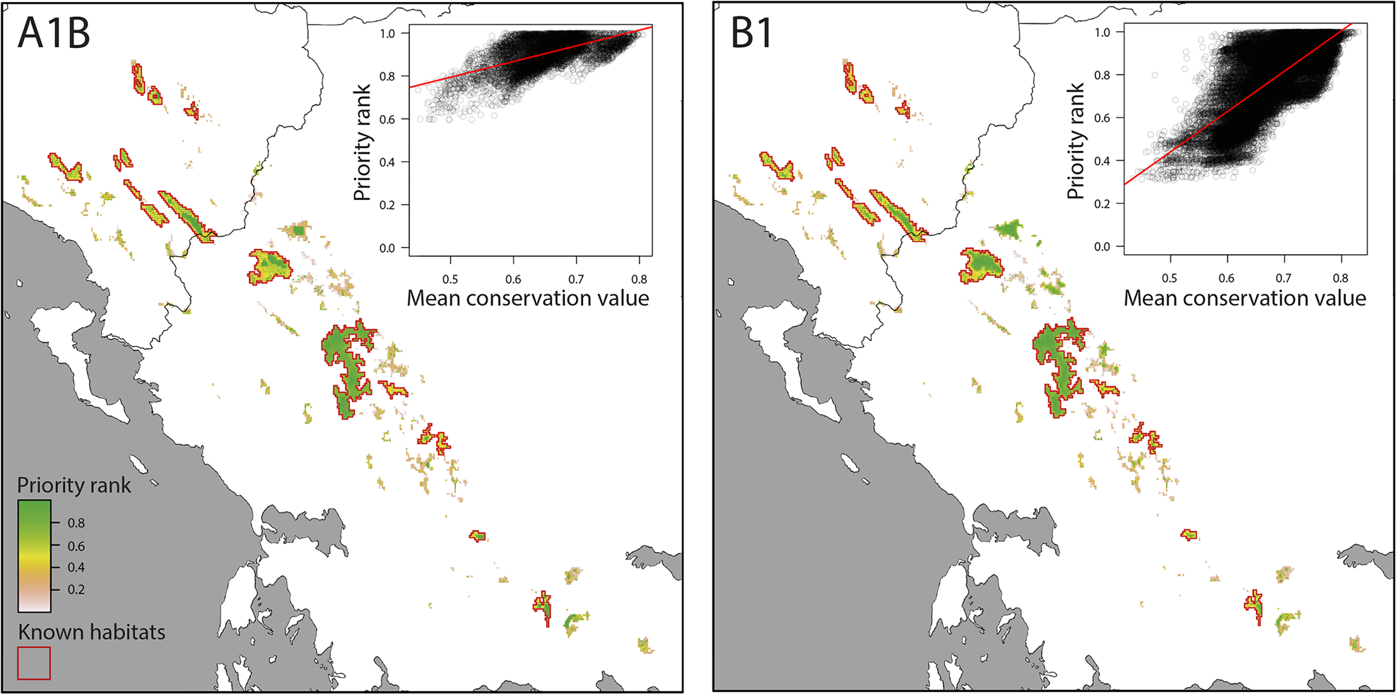
Fig. 3 Spatial conservation priorities for pessimistic (A1B) and optimistic (B1) future climate scenarios (main panels) and linear regression of priority rank over mean conservation value per cell (insets).

Fig. 4 Key areas for the persistence of V. graeca populations and their inclusion in protected areas in pessimistic (A1B) and optimistic (B1) future climate scenarios. SCI, Site of community importance (EU Natura 2000 Habitats Directive site); SPA, Special protection area (EU Natura 2000 Birds Directive site).
Current protection
Protected areas covered 13.3% of the area known to hold V. graeca populations in Albania and 90.6% in Greece (Fig. 4). Under the A1B scenario, the total area of high-priority cells covered by protected areas was 242.7 km2, or 81.8% of the high-priority areas that are protected, but none of the high priority areas were located in protected areas in Albania and all high priority areas were in protected areas in Greece (Fig. 4). Under the B1 scenario the total protected high priority area was 221.2 km2 or 83.5% of all high priority areas, all of which were in Greece (Fig. 4, Table 1).
Table 1 Areas of high-priority landscapes predicted by spatial prioritization under two climate scenarios (A1B, B2) until 2080 for the conservation of Vipera graeca and that are covered by various categories of the current network of protected areas.

Interrelationships of conservation value variables
Cluster analysis revealed four clusters of conservation value variables (Fig. 5). Habitat alteration was mostly independent of other variables. Vegetation suitability was clustered with disturbance and habitat degradation, and climate suitability was related to habitat size. Population persistence was closely related to the opportunity of altitudinal shift (r = 0.64, r = 0.73 for A1B and B1, respectively). No site had maximum conservation value for all variables.
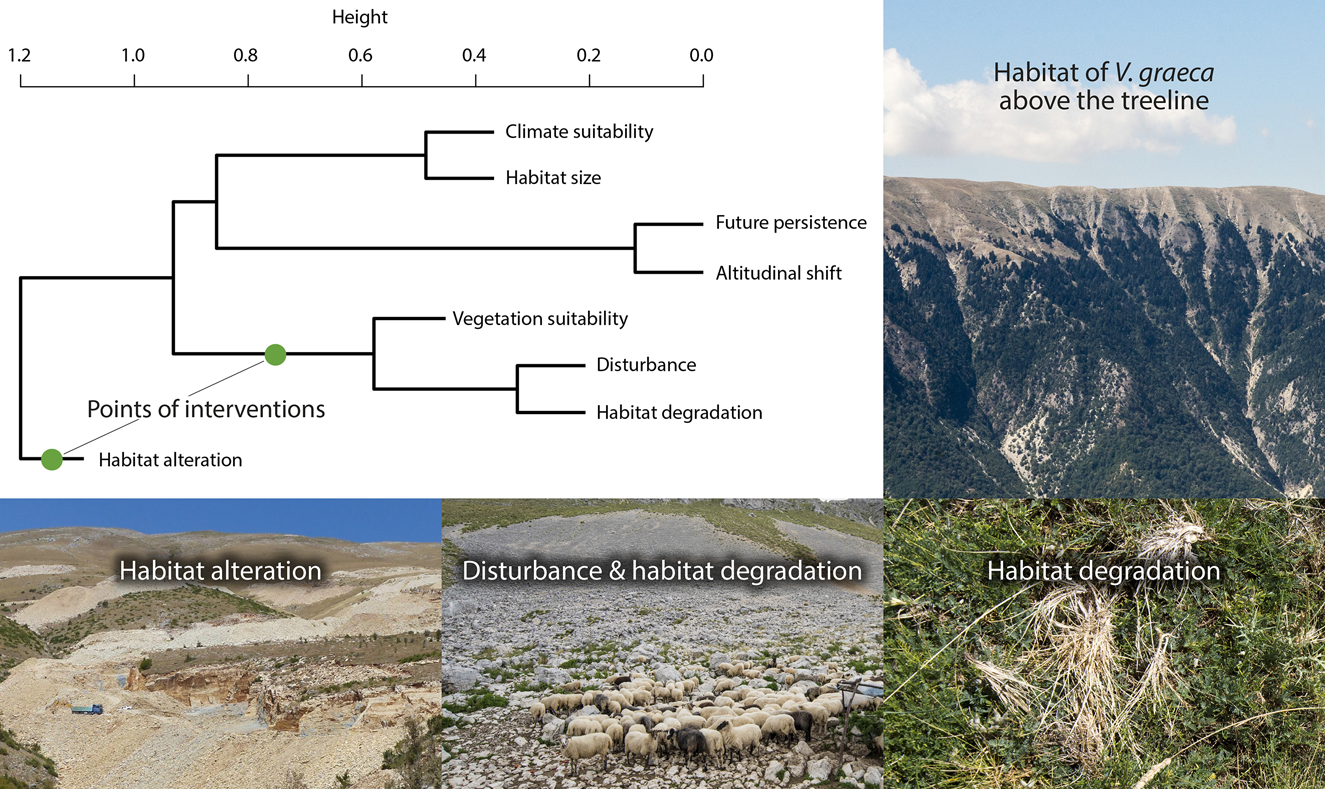
Fig. 5 Agglomerative hierarchical clustering of conservation value layers and illustrations of the habitat of V. graeca and the most important threats. Conservation management actions should be targeted at the points of interventions. Note that the binary habitat occupancy variable is not included.
Discussion
Our study provides four main results. Firstly, the modelling of future climatic conditions showed a significant 81–90% reduction in the area of habitats suitable for V. graeca by the end of the 2080s. Secondly, current protection appears adequate for the persistence of the species in Greece but not in Albania. Thirdly, conservation efforts are most likely to succeed if they target habitat alteration, degradation and disturbance as these have similar effects and the other threats are not easy to address at local scales (Fig. 5). Fourthly, our approach shows that threats can be mapped and used to estimate the conservation value of areas, which can then be used in spatial conservation prioritization for single species.
Expected impact of climate change
Our analyses support the previous results of Mizsei et al. (Reference Mizsei, Üveges, Vági, Szabolcs, Lengyel and Pfliegler2016) showing that the distribution of V. graeca is limited to the coldest and highest elevation habitats in the Southern Balkans. However, based on future climate scenarios, there will not be any remaining suitable habitats (i.e. with mean annual temperature < 10 °C ) in the Southern Balkans by 2100 within the current range of the species (Lelieveld et al., Reference Lelieveld, Hadjinicolaou, Kostopoulo, Chenoweth, El Maayar and Giannakopoulos2012). Thus, the probability of the extinction of V. graeca is high, as unassisted long-distance dispersal to other high elevation mountains that may be suitable in the future is not possible. Besides increases in temperature, substantial aridification is expected throughout the Mediterranean basin (Foufopoulos & Ives, Reference Foufopoulos and Ives1999). Precipitation quantity and frequency are predicted to decrease and the number of dry days is predicted to increase considerably by 2100 (Lelieveld et al., Reference Lelieveld, Hadjinicolaou, Kostopoulo, Chenoweth, El Maayar and Giannakopoulos2012; Mariotti et al., Reference Mariotti, Pan, Zeng and Alessandri2015). For ectotherms, a change in the thermal landscape will probably reduce the time available for daily activity, which will affect foraging, feeding and breeding success (Walther et al., Reference Walther, Post, Convey, Menzel, Parmesan and Beebee2002). For a cold-adapted species such as V. graeca, these changes will have an impact on the persistence of the species as it already occupies a narrow niche in a harsh environment.
Novelties and limitations in estimating land use impact
Our approach involved two rarely used methods. Our layer for habitat degradation characterized grazing pressure by the decrease in phytomass between spring and autumn, which adequately represents grazing pressure in grasslands (Todd et al., Reference Todd, Hoffer and Milchunas1998; Senay & Elliott, Reference Senay and Elliott2000; Kawamura et al., Reference Kawamura, Akiyama, Yokota, Tsutsumi, Yasuda, Watanabe and Wang2005). We developed this further by spatial interpolation of the distribution of livestock folds weighted by phytomass decrease, which is a novel approach to estimating the intensity of land use or the degree of disturbance. Further studies are needed to calibrate this type of derived variable accurately with on-site measurements or experiments.
One potential limitation of our study is that land-use intensity is probably higher at the lower elevations of V. graeca habitats (1,500–1,800 m) than at higher elevations. Lower elevations are easier to access for people and grazing livestock, snow melts are earlier, and thus the grazing season is longer than at higher elevations. Therefore it is possible that V. graeca may already have disappeared from lower elevations as a result of anthropogenic impacts, and that our suitability models based on current conditions are biased to colder climates and/or higher elevations. This is unlikely, however, because lower elevations are often secondary grasslands established in previously wooded areas below the former treeline, as evidenced by wooded areas remaining on slopes too steep for grazing livestock (Fig. 5). It is therefore unlikely that these lower elevation areas were formerly suitable for V. graeca. Moreover, overgrazing also occurs at higher elevations, where the species is present, albeit in lower abundance. Nevertheless, because the species was discovered only in the 1980s there are no historical data to test temporal patterns in habitat occupancy.
Prioritization for single species
Systematic conservation planning techniques were developed for multiple species (Lehtomäki & Moilanen, Reference Lehtomäki and Moilanen2013) and have only recently been applied for single species (Adam-Hosking et al., Reference Adam-Hosking, McAlpine, Rhodes, Moss and Grantham2015). Single species conservation planning follows the same protocol but ranks sites according to the spatial distribution of threat factors (or conservation value), and/or the cost of protection (Adams-Hosking et al., Reference Adam-Hosking, McAlpine, Rhodes, Moss and Grantham2015; Nori et al., Reference Nori, Torres, Lescano, Cordier, Periago and Baldo2016). The scarcity of systematic conservation planning for single species is probably a result of the primary importance of biodiversity protection as opposed to species protection. Our study shows that the approach can provide information of value for the conservation of umbrella, flagship or keystone species.
Recommendations for the conservation of V. graeca
Our study shows that V. graeca habitats may face significant losses or further fragmentation up to 2089, although some populations in a few contiguous habitats are predicted to persist. These results suggest that conservation should focus on sites of high importance by improving habitat quality, reducing disturbance and degradation, effectively protecting the species, educating local stakeholders and continuing to monitor the populations.
Raising awareness and involvement of local communities is central to any conservation action, to ensure its success, and to establish sustainable land use (Adele et al., Reference Adele, Stevens and Bridgewater2015). Research by the Greek Meadow Viper Working Group on human–wildlife conflict resulting from sheep mortality as a result of snake bites is already underway and is trying to identify ways to involve local communities. This project has already recommended that shepherds follow two guidelines for grazing livestock in V. graeca habitats: avoid grazing on south-eastern slopes where vipers are more abundant, or, if the shepherd must utilize these slopes, do so between 11.00–15.00, when vipers usually shelter from the midday heat.
Our findings warrant slightly different recommendations for sustainable land use in the two countries. In Albania grazing pressure needs to be reduced to achieve an improved, more natural vegetation structure in meadows. In Greece a shift from cattle grazing to sheep grazing is required. Cattle grazing has a stronger and more negative impact because cattle uproot vegetation, which is detrimental to both the top soil layer and vegetation. Eradication of fescue tussocks (Fig. 5) has already changed the vegetation, resulting in the homogenization of microhabitats: there are fewer structures that provide shelter and shade for snakes, which in turn increases predation by birds of prey and reduces the abundance of the viper's Orthopteran prey (Lemonnier-Darcemont et al., Reference Lemonnier-Darcemont, Kati, Willemse and Darcemont2018).
Along with habitat conservation, we recommend the launch of an ex situ breeding programme, similar to that for the threatened Hungarian meadow viper Vipera ursinii rakosiensis (Péchy et al., Reference Péchy, Halpern, Sós and Walzer2015), to help reinforce populations that are suffering from the symptoms of an extinction vortex. We suggest that a combination of ex situ and in situ conservation plans and continued research on the ecology and population genetics of V. graeca in high priority areas are necessary to ensure persistence. Further research, in conjunction with local and governmental support, is key for the development of a species conservation programme that will ensure the long-term survival of this Endangered, cold-adapted species trapped on mountaintops in the warming Mediterranean basin.
Acknowledgements
Financial support was provided by the Mohamed bin Zayed Species Conservation Fund (no. 150510498), Rufford Small Grant (no. 15478-1), Chicago Zoological Society's Chicago Board of Trade Endangered Species Fund, Campus Hungary (no. B2/1CS/19196/9), ERASMUS+, the Visegrad Scholarship and two grants from the National Research, Development and Innovation Office of Hungary (NKFIH-OTKA K106133, GINOP 2.3.3-15-2016-00019). Permits for fieldwork were provided by the Ministry for Environment and Energy of Greece (number 158977/1757) and the Ministry of Environment of Albania (number 6584).
Author contributions
Study design: EM, MS, SL; collection and processing of spatial data: EM, LS, ZB, KM; collection of field data: EM, MS, SAR, MD, ZB, SL, YI; data analysis: EM, ZV; writing: EM, MS, SAR; contribution to writing: all authors.
Conflicts of interest
None.
Ethical standards
This research abided by the Oryx guidelines on ethical standards. Individual snakes were not collected or harmed in any way in the course of this study.
Data accessibility
The R script of conservation value layers and the produced ASCII files are available as supplementary material. Occurrence data are not provided, to protect the species, but are available for bona fide researchers upon request from the corresponding author.


 Open access