


1 Introduction
Studies of the turbulent transport of mass, momentum and energy have composed a significant fraction of plasma physics research over the last half-century. Of particular interest is the question of what mechanisms extract energy from the turbulent cascade, damping electromagnetic fluctuations and eventually irreversibly heating the plasma. The answer to this question will improve the understanding of a wide array of plasma systems, ranging from laboratory devices, planetary magnetospheres, the Sun and its extended atmosphere and accretion disks around massive astrophysical bodies.
Proposed mechanisms for the dissipation of turbulence in weakly collisional plasmas can broadly be grouped into three classes: resonant mechanisms, such as Landau damping, transit-time damping or cyclotron damping (Landau Reference Landau1946; Barnes Reference Barnes1966; Coleman Reference Coleman1968; Denskat, Beinroth & Neubauer Reference Denskat, Beinroth and Neubauer1983; Isenberg & Hollweg Reference Isenberg and Hollweg1983; Goldstein, Roberts & Fitch Reference Goldstein, Roberts and Fitch1994; Leamon et al. Reference Leamon, Smith, Ness, Matthaeus and Wong1998; Quataert Reference Quataert1998; Gary Reference Gary1999; Hollweg & Isenberg Reference Hollweg and Isenberg2002; TenBarge & Howes Reference TenBarge and Howes2013); non-resonant mechanisms, such as the stochastic heating of ions in large amplitude, low-frequency Alfvénic turbulence (McChesney, Stern & Bellan Reference McChesney, Stern and Bellan1987; Chen, Lin & White Reference Chen, Lin and White2001; Johnson & Cheng Reference Johnson and Cheng2001; Bourouaine, Marsch & Vocks Reference Bourouaine, Marsch and Vocks2008; Chandran Reference Chandran2010; Chandran et al. Reference Chandran, Li, Rogers, Quataert and Germaschewski2010; Bourouaine & Chandran Reference Bourouaine and Chandran2013); and intermittent dissipation in current sheets and magnetic reconnection sites (Dmitruk, Matthaeus & Seenu Reference Dmitruk, Matthaeus and Seenu2004; Markovskii & Vasquez Reference Markovskii and Vasquez2011; Matthaeus & Velli Reference Matthaeus and Velli2011; Servidio et al. Reference Servidio, Greco, Matthaeus, Osman and Dmitruk2011; Karimabadi et al. Reference Karimabadi, Roytershteyn, Wan, Matthaeus, Daughton, Wu, Shay, Loring, Borovsky and Leonardis2013; Zhdankin et al. Reference Zhdankin, Uzdensky, Perez and Boldyrev2013; Osman et al. Reference Osman, Kiyani, Chapman and Hnat2014a ,Reference Osman, Matthaeus, Gosling, Greco, Servidio, Hnat, Chapman and Phan b ; Zhdankin, Uzdensky & Boldyrev Reference Zhdankin, Uzdensky and Boldyrev2015). All three classes couple electromagnetic fluctuations to the plasma particle velocity distribution, leading to energy transfer and damping. This coupling occurs through the nonlinear wave–particle interaction term in the Vlasov equation (Howes Reference Howes2015; Howes, Klein & Li Reference Howes, Klein and Li2017). Each mechanism produces distinct structures in velocity space that are characteristic of that mechanism. For example, resonant mechanisms preferentially energize particles near a resonant velocity with a change in sign in the energy transfer across that resonant velocity, while the stochastic heating described by Chandran et al. (Reference Chandran, Li, Rogers, Quataert and Germaschewski2010) will only energize thermal and sub-thermal particles, producing a platykurtic distribution (Klein & Chandran Reference Klein and Chandran2016).
The solar wind, a low-density and high-temperature plasma accelerated from the Sun that flows radially outward through the heliosphere, is a heavily sampled space plasma system, with measurements dating back to the dawn of the space age. The large quantity of measurements of this super-Alfvénic plasma flow makes it a unique system with which various plasma and turbulence theories, including descriptions of damping and dissipation, can be tested across a wide range of physical scales and plasma parameters. A significant limitation of such in situ measurements is that most observations occur at a single point, or at most a few points, in space. Any attempts to use the solar wind to test theories of turbulence must take this limitation into consideration.
A novel field–particle correlation technique has been proposed (Klein & Howes Reference Klein and Howes2016; Howes et al. Reference Howes, Klein and Li2017) which uses single-point measurements to capture the non-oscillatory, or secular, transfer of energy associated with the net removal of energy from turbulent fluctuations. This correlation isolates the secular energy transfer by averaging the nonlinear field–particle interaction term in the Vlasov equation over a time interval longer than the time scale characteristic of the turbulent fluctuations involved in the energy transfer. Crucially, not only can the secular energy transfer be isolated, but the velocity-space structure of this correlation can be used to discriminate between various collisionless damping mechanisms using only single-point measurements of the type accessible to spacecraft in the solar wind.
A fundamental question at the forefront of heliophysics research is whether Landau damping, and other resonant wave–particle interactions, can effectively remove energy from turbulent plasmas given the highly nonlinear nature of strong plasma turbulence (Plunk Reference Plunk2013; Schekochihin et al. Reference Schekochihin, Parker, Highcock, Dellar, Dorland and Hammett2016). In this work, we seek evidence of Landau damping in turbulent plasmas by the application of field–particle correlations to data extracted from a series of gyrokinetic simulations of three-dimensional electromagnetic plasma turbulence. This extends previous work applying such correlations to monochromatic, electrostatic waves (Klein & Howes Reference Klein and Howes2016; Howes et al. Reference Howes, Klein and Li2017; Klein Reference Klein2017) and the Landau damping of a single kinetic Alfvén wave (Howes Reference Howes2017) to a system of strong turbulence where the role of resonant interactions is a matter of current debate.
The remainder of this paper is organized as follows. The electromagnetic form of the field–particle correlation is developed in § 2. A presentation of the expected structure of damping in low-frequency turbulence is found in § 3, followed by a discussion of the simulation code employed, AstroGK, in § 4. In § 5, we apply the correlation to a single kinetic Alfvén wave, followed by an application to turbulent simulations in § 6. Discussion, summary and future applications are found in § 7. Even in the presence of strong turbulence and spatially inhomogeneous heating, the secular energy transfer from the turbulent fields to the protons is shown to be localized in velocity space near the resonant velocities associated with Landau damping. This work motivates future application to data from turbulence simulations which contain other damping mechanisms, as well as spacecraft observations, with the ultimate goal to determine which mechanisms act to dissipate turbulence in the solar wind.
2 Field–particle correlations for electromagnetic fluctuations
The novel approach of using field–particle correlations to diagnose the energy transfer between fields and particles has been described for electrostatic fluctuations in the Vlasov–Poisson system (Howes et al. Reference Howes, Klein and Li2017) and been applied to both damped and linearly unstable systems (Klein & Howes Reference Klein and Howes2016; Howes Reference Howes2017; Klein Reference Klein2017). Here we describe the application of the field–particle correlation technique to the case of electromagnetic fluctuations in the Vlasov–Maxwell system.
The Boltzmann equation describes the dynamics and energetics of weakly collisional plasmas relevant to heliospheric environments, such as the solar corona and the solar wind, determining the evolution of the six-dimensional velocity distribution function
 $f_{s}(\boldsymbol{r},\boldsymbol{v},t)$
for a plasma species
$f_{s}(\boldsymbol{r},\boldsymbol{v},t)$
for a plasma species
 $s$
,
$s$
,
 $$\begin{eqnarray}\frac{\unicode[STIX]{x2202}f_{s}}{\unicode[STIX]{x2202}t}+\boldsymbol{v}\boldsymbol{\cdot }\unicode[STIX]{x1D735}f_{s}+\frac{q_{s}}{m_{s}}\left[\boldsymbol{E}+\frac{\boldsymbol{v}\times \boldsymbol{B}}{c}\right]\boldsymbol{\cdot }\frac{\unicode[STIX]{x2202}f_{s}}{\unicode[STIX]{x2202}\boldsymbol{v}}=\left(\frac{\unicode[STIX]{x2202}f_{s}}{\unicode[STIX]{x2202}t}\right)_{\text{coll}}.\end{eqnarray}$$
The species charge and mass are
 $q_{s}$
and
$q_{s}$
and
 $m_{s}$
respectively,
$m_{s}$
respectively,
 $\boldsymbol{v}$
the velocity,
$\boldsymbol{v}$
the velocity,
 $\boldsymbol{E}$
and
$\boldsymbol{E}$
and
 $\boldsymbol{B}$
the electric and magnetic fields, and
$\boldsymbol{B}$
the electric and magnetic fields, and
 $c$
the speed of light. Combining the Boltzmann equation for each plasma species together with Maxwell’s equations forms the closed set of Maxwell–Boltzmann equations that govern the nonlinear evolution of turbulent fluctuations in a magnetized kinetic plasma.
$c$
the speed of light. Combining the Boltzmann equation for each plasma species together with Maxwell’s equations forms the closed set of Maxwell–Boltzmann equations that govern the nonlinear evolution of turbulent fluctuations in a magnetized kinetic plasma.
Here we focus strictly on the collisionless dynamics of the energy transfer between fields and particles, so we drop the collision operator on the right-hand side of (2.1) to obtain the Vlasov equation. Multiplying the Vlasov equation by
 $m_{s}v^{2}/2$
, integrating over all position and velocity space, and using an integration by parts in velocity for the Lorentz force term yields the expression
$m_{s}v^{2}/2$
, integrating over all position and velocity space, and using an integration by parts in velocity for the Lorentz force term yields the expression
 $$\begin{eqnarray}\frac{\unicode[STIX]{x2202}W_{s}}{\unicode[STIX]{x2202}t}=\int \text{d}^{3}\boldsymbol{r}\int \text{d}^{3}\boldsymbol{v}q_{s}\boldsymbol{v}\boldsymbol{\cdot }\boldsymbol{E}f_{s}=\int \text{d}^{3}\boldsymbol{r}\boldsymbol{j}_{s}\boldsymbol{\cdot }\boldsymbol{E},\end{eqnarray}$$
where the current density of species
 $s$
is defined as
$s$
is defined as
 $\boldsymbol{j}_{s}\equiv \int \text{d}^{3}\boldsymbol{v}q_{s}\boldsymbol{v}f_{s}$
and the microscopic particle kinetic energy for species
$\boldsymbol{j}_{s}\equiv \int \text{d}^{3}\boldsymbol{v}q_{s}\boldsymbol{v}f_{s}$
and the microscopic particle kinetic energy for species
 $s$
is given by
$s$
is given by
 $$\begin{eqnarray}W_{s}\equiv \int \text{d}^{3}\boldsymbol{r}\int \text{d}^{3}\boldsymbol{v}\frac{1}{2}m_{s}v^{2}f_{s}(\boldsymbol{r},\boldsymbol{v},t).\end{eqnarray}$$
Note that the ballistic term (the second term on the left-hand side of (2.1)) and the magnetic part of the Lorentz term (the third term on the left-hand side) yield zero net energy transfer upon integration over all position and velocity space, assuming suitable boundary conditions, such as periodic boundaries or infinitely distant boundaries with vanishing
 $f_{s}$
. Summing (2.2) over species and combining with Poynting’s theorem
$f_{s}$
. Summing (2.2) over species and combining with Poynting’s theorem
 $$\begin{eqnarray}\frac{\unicode[STIX]{x2202}}{\unicode[STIX]{x2202}t}\int \text{d}^{3}\boldsymbol{r}\frac{|\boldsymbol{E}|^{2}+|\boldsymbol{B}|^{2}}{8\unicode[STIX]{x03C0}}+\frac{c}{4\unicode[STIX]{x03C0}}\oint \text{d}^{2}\boldsymbol{S}\boldsymbol{\cdot }(\boldsymbol{E}\times \boldsymbol{B})=-\int \text{d}^{3}\boldsymbol{r}\boldsymbol{j}\boldsymbol{\cdot }\boldsymbol{E},\end{eqnarray}$$
where
 $\boldsymbol{j}=\sum _{s}\boldsymbol{j}_{s}$
is the total current density, we may obtain the conserved Vlasov–Maxwell energy,
$\boldsymbol{j}=\sum _{s}\boldsymbol{j}_{s}$
is the total current density, we may obtain the conserved Vlasov–Maxwell energy,
 $W$
, for electromagnetic fluctuations in a collisionless, magnetized plasma,
$W$
, for electromagnetic fluctuations in a collisionless, magnetized plasma,
 $$\begin{eqnarray}W=\int \text{d}^{3}\boldsymbol{r}\frac{|\boldsymbol{E}|^{2}+|\boldsymbol{B}|^{2}}{8\unicode[STIX]{x03C0}}+\mathop{\sum }_{s}\int \text{d}^{3}\boldsymbol{r}\int \text{d}^{3}\boldsymbol{v}\frac{1}{2}m_{s}v^{2}f_{s}.\end{eqnarray}$$
Note that, for periodic or infinitely distant boundaries, the Poynting flux term, the second term on the left-hand side of (2.4), yields zero net change in the energy
 $W$
.
$W$
.
In the Vlasov–Maxwell system, equation (2.2) shows clearly that the change in the microscopic energy of the particles is accomplished by interactions of the particles with the electric field, where
 $\boldsymbol{j}_{s}\boldsymbol{\cdot }\boldsymbol{E}$
is the (spatially) local rate of change of the energy density of particle species
$\boldsymbol{j}_{s}\boldsymbol{\cdot }\boldsymbol{E}$
is the (spatially) local rate of change of the energy density of particle species
 $s$
. But, as pointed out in the previous description of how to use field–particle correlations to explore the conversion of turbulent energy into microscopic particle energy (Howes et al.
Reference Howes, Klein and Li2017), this energy transfer between fields and particles includes both the conservative oscillating energy transfer associated with undamped wave motion and the secular energy transfer associated with the collisionless damping of the turbulent fluctuations. Here we specifically define the turbulence as the sum of the fluctuations in the electromagnetic fields and the fluctuations of the bulk flows of the plasma (Howes Reference Howes2015). Collisionless interactions between the fields and the particles, governed by the Lorentz force term (third term on the left-hand side) in (2.1), remove the energy from the turbulent fluctuations, transferring it into microscopic particle kinetic energy that is not associated with bulk plasma motions. Diagnosing this net transfer of energy between fields and particles is the key aim of the field–particle correlation method, using a time average over an appropriately chosen correlation interval to eliminate the often large signal of the oscillating energy transfer, exposing the smaller signal of the secular energy transfer.
$s$
. But, as pointed out in the previous description of how to use field–particle correlations to explore the conversion of turbulent energy into microscopic particle energy (Howes et al.
Reference Howes, Klein and Li2017), this energy transfer between fields and particles includes both the conservative oscillating energy transfer associated with undamped wave motion and the secular energy transfer associated with the collisionless damping of the turbulent fluctuations. Here we specifically define the turbulence as the sum of the fluctuations in the electromagnetic fields and the fluctuations of the bulk flows of the plasma (Howes Reference Howes2015). Collisionless interactions between the fields and the particles, governed by the Lorentz force term (third term on the left-hand side) in (2.1), remove the energy from the turbulent fluctuations, transferring it into microscopic particle kinetic energy that is not associated with bulk plasma motions. Diagnosing this net transfer of energy between fields and particles is the key aim of the field–particle correlation method, using a time average over an appropriately chosen correlation interval to eliminate the often large signal of the oscillating energy transfer, exposing the smaller signal of the secular energy transfer.
A significant limitation of spacecraft measurements is that information is generally limited to a single point, or at most a few points, in space. Therefore, the spatial integration necessary to simplify the energy transfer in the Vlasov equation to the form given by (2.2) is not possible. To explore the energy transfer between fields and particles at a single point in space, we define the phase-space energy density for a particle species
 $s$
by
$s$
by
 $w_{s}(\boldsymbol{r},\boldsymbol{v},t)=m_{s}v^{2}f_{s}(\boldsymbol{r},\boldsymbol{v},t)/2$
. Multiplying the Vlasov equation by
$w_{s}(\boldsymbol{r},\boldsymbol{v},t)=m_{s}v^{2}f_{s}(\boldsymbol{r},\boldsymbol{v},t)/2$
. Multiplying the Vlasov equation by
 $m_{s}v^{2}/2$
, but not integrating over space or velocity, we obtain an expression for the rate of change of the phase-space energy density,
$m_{s}v^{2}/2$
, but not integrating over space or velocity, we obtain an expression for the rate of change of the phase-space energy density,
 $$\begin{eqnarray}\frac{\unicode[STIX]{x2202}w_{s}(\boldsymbol{r},\boldsymbol{v},t)}{\unicode[STIX]{x2202}t}=-\boldsymbol{v}\boldsymbol{\cdot }\unicode[STIX]{x1D735}w_{s}-q_{s}\frac{v^{2}}{2}\boldsymbol{E}\boldsymbol{\cdot }\frac{\unicode[STIX]{x2202}f_{s}}{\unicode[STIX]{x2202}\boldsymbol{v}}-\frac{q_{s}}{c}\frac{v^{2}}{2}(\boldsymbol{v}\times \boldsymbol{B})\boldsymbol{\cdot }\frac{\unicode[STIX]{x2202}f_{s}}{\unicode[STIX]{x2202}\boldsymbol{v}}.\end{eqnarray}$$
When integrated over velocity space, an integration by parts of the last term on the right-hand side of (2.6) yields an integrand containing
 $\boldsymbol{v}\boldsymbol{\cdot }(\boldsymbol{v}\times \boldsymbol{B})=0$
, so the magnetic field cannot accomplish any net change of energy of the particles. In addition, when integrated over volume, the first term on the right-hand side of (2.6) yields zero net energy change for either periodic or infinite boundary conditions. Therefore, we focus here on the second term on the right-hand side of (2.6), the term that determines the effect of the electric field on the rate of change of phase-space energy density.Footnote
1
$\boldsymbol{v}\boldsymbol{\cdot }(\boldsymbol{v}\times \boldsymbol{B})=0$
, so the magnetic field cannot accomplish any net change of energy of the particles. In addition, when integrated over volume, the first term on the right-hand side of (2.6) yields zero net energy change for either periodic or infinite boundary conditions. Therefore, we focus here on the second term on the right-hand side of (2.6), the term that determines the effect of the electric field on the rate of change of phase-space energy density.Footnote
1
Examining the electric field term, we can write the form of the field–particle correlation at a single point
 $\boldsymbol{r}_{0}$
for the general Vlasov–Maxwell case, separating the contributions from the parallel and perpendicular parts of the electric field,
$\boldsymbol{r}_{0}$
for the general Vlasov–Maxwell case, separating the contributions from the parallel and perpendicular parts of the electric field,
 $$\begin{eqnarray}\displaystyle & \displaystyle C_{E_{\Vert }}(\boldsymbol{v},t,\unicode[STIX]{x1D70F})=C\left(-q_{s}\frac{v_{\Vert }^{2}}{2}\frac{\unicode[STIX]{x2202}f_{s}(\boldsymbol{r}_{0},\boldsymbol{v},t)}{\unicode[STIX]{x2202}v_{\Vert }},E_{\Vert }(\boldsymbol{r}_{0},t)\right) & \displaystyle\end{eqnarray}$$
 $$\begin{eqnarray}\displaystyle & \displaystyle C_{E_{\bot }}(\boldsymbol{v},t,\unicode[STIX]{x1D70F})=C\left(-q_{s}\frac{v_{x}^{2}}{2}\frac{\unicode[STIX]{x2202}f_{s}(\boldsymbol{r}_{0},\boldsymbol{v},t)}{\unicode[STIX]{x2202}v_{x}},E_{x}(\boldsymbol{r}_{0},t)\right)+C\left(-q_{s}\frac{v_{y}^{2}}{2}\frac{\unicode[STIX]{x2202}f_{s}(\boldsymbol{r}_{0},\boldsymbol{v},t)}{\unicode[STIX]{x2202}v_{y}},E_{y}(\boldsymbol{r}_{0},t)\right), & \displaystyle \nonumber\\ \displaystyle & & \displaystyle\end{eqnarray}$$
where we define the non-normalized correlation
 $$\begin{eqnarray}C(A,B)\equiv \frac{1}{N}\mathop{\sum }_{j=i}^{i+N}A_{j}B_{j}\end{eqnarray}$$
for quantities
 $A$
and
$A$
and
 $B$
measured at discrete times
$B$
measured at discrete times
 $t_{j}=j\unicode[STIX]{x0394}t$
with correlation interval
$t_{j}=j\unicode[STIX]{x0394}t$
with correlation interval
 $\unicode[STIX]{x1D70F}\equiv N\unicode[STIX]{x0394}t$
. Note that the
$\unicode[STIX]{x1D70F}\equiv N\unicode[STIX]{x0394}t$
. Note that the
 $v^{2}=v_{\Vert }^{2}+v_{\bot }^{2}$
factor is reduced to
$v^{2}=v_{\Vert }^{2}+v_{\bot }^{2}$
factor is reduced to
 $v_{\Vert }^{2}$
for
$v_{\Vert }^{2}$
for
 $C_{E_{\Vert }}$
because the net energy change is zero for the
$C_{E_{\Vert }}$
because the net energy change is zero for the
 $v_{\bot }^{2}$
contribution when integrated over velocity. Similarly, for
$v_{\bot }^{2}$
contribution when integrated over velocity. Similarly, for
 $C_{E_{\bot }}$
, one uses
$C_{E_{\bot }}$
, one uses
 $v_{x}^{2}$
for the energy change due to
$v_{x}^{2}$
for the energy change due to
 $E_{x}$
and
$E_{x}$
and
 $v_{y}^{2}$
for the energy change due to
$v_{y}^{2}$
for the energy change due to
 $E_{y}$
, where we assume for notational simplicity that the local magnetic field is in the
$E_{y}$
, where we assume for notational simplicity that the local magnetic field is in the
 $\hat{\boldsymbol{z}}$
direction,
$\hat{\boldsymbol{z}}$
direction,
 $\boldsymbol{B}=B(r_{0})\hat{\boldsymbol{z}}$
.
$\boldsymbol{B}=B(r_{0})\hat{\boldsymbol{z}}$
.
Note that, depending on the physical mechanism to be investigated, one will choose the appropriate correlation, either
 $C_{E_{\Vert }}$
or
$C_{E_{\Vert }}$
or
 $C_{E_{\bot }}$
. One would choose
$C_{E_{\bot }}$
. One would choose
 $C_{E_{\Vert }}$
to investigate Landau damping, since it is mediated by the parallel electric field, and one would choose
$C_{E_{\Vert }}$
to investigate Landau damping, since it is mediated by the parallel electric field, and one would choose
 $C_{E_{\bot }}$
to study cyclotron damping or stochastic ion heating, since these mechanisms are mediated by the perpendicular electric field. Importantly, regardless of the underlying mechanism,
$C_{E_{\bot }}$
to study cyclotron damping or stochastic ion heating, since these mechanisms are mediated by the perpendicular electric field. Importantly, regardless of the underlying mechanism,
 $C_{E_{\Vert }}$
and
$C_{E_{\Vert }}$
and
 $C_{E_{\bot }}$
measure the energy density transfer mediated by the associated electric field component.
$C_{E_{\bot }}$
measure the energy density transfer mediated by the associated electric field component.
Since taking the velocity gradient of noisy or low resolution phase-space measurements of particle velocity distribution functions can lead to large errors, one can define a related correlation
 $C^{\prime }$
that is derived by an integration by parts in velocity (Howes et al.
Reference Howes, Klein and Li2017). These alternative forms are
$C^{\prime }$
that is derived by an integration by parts in velocity (Howes et al.
Reference Howes, Klein and Li2017). These alternative forms are
 $$\begin{eqnarray}\displaystyle & \displaystyle C_{E_{\Vert }}^{\prime }(\boldsymbol{v},t,\unicode[STIX]{x1D70F})=C(q_{s}v_{\Vert }\,f_{s}(\boldsymbol{r}_{0},\boldsymbol{v},t),E_{\Vert }(\boldsymbol{r}_{0},t)) & \displaystyle\end{eqnarray}$$
 $$\begin{eqnarray}\displaystyle & \displaystyle C_{E_{\bot }}^{\prime }(\boldsymbol{v},t,\unicode[STIX]{x1D70F})=C(q_{s}v_{x}\,f_{s}(\boldsymbol{r}_{0},\boldsymbol{v},t),E_{x}(\boldsymbol{r}_{0},t))+C(q_{s}v_{y}\,f_{s}(\boldsymbol{r}_{0},\boldsymbol{v},t),E_{y}(\boldsymbol{r}_{0},t)). & \displaystyle\end{eqnarray}$$
When integrated over velocity,
 $C_{E_{\Vert }}^{\prime }$
simply yields the time averaged
$C_{E_{\Vert }}^{\prime }$
simply yields the time averaged
 $j_{s\Vert }E_{\Vert }$
and
$j_{s\Vert }E_{\Vert }$
and
 $C_{E_{\bot }}^{\prime }$
yields the time averaged
$C_{E_{\bot }}^{\prime }$
yields the time averaged
 $\boldsymbol{j}_{s\bot }\boldsymbol{\cdot }\boldsymbol{E}_{\bot }$
, which is the net electromagnetic work done on the particles. And since the alternative forms
$\boldsymbol{j}_{s\bot }\boldsymbol{\cdot }\boldsymbol{E}_{\bot }$
, which is the net electromagnetic work done on the particles. And since the alternative forms
 $C^{\prime }$
are equivalent to the
$C^{\prime }$
are equivalent to the
 $C$
forms of the field–particle correlations when integrated over velocity, the original forms
$C$
forms of the field–particle correlations when integrated over velocity, the original forms
 $C$
given by (2.7) and (2.8) also yield, upon velocity integration, the net electromagnetic work done on the particles.
$C$
given by (2.7) and (2.8) also yield, upon velocity integration, the net electromagnetic work done on the particles.
3 Resonant energy transfer in low-frequency turbulence
We next describe the damping mechanisms accessible to turbulence in solar and astrophysical plasmas and predict where in velocity space the related energy transfer is expected to appear. The resonant mechanisms that can remove energy from weakly collisional plasma turbulence depend strongly on the frequency of the turbulent fluctuations. Direct multi-spacecraft observations of the solar wind find that turbulent fluctuations at length scales near ion kinetic scales are anisotropic, with
 $k_{\bot }\gg k_{\Vert }$
, with
$k_{\bot }\gg k_{\Vert }$
, with
 $\bot$
and
$\bot$
and
 $\Vert$
defined with respect to the local mean magnetic field (Sahraoui et al.
Reference Sahraoui, Belmont, Goldstein and Rezeau2010; Narita et al.
Reference Narita, Gary, Saito, Glassmeier and Motschmann2011; Roberts, Li & Li Reference Roberts, Li and Li2013; Roberts, Li & Jeska Reference Roberts, Li and Jeska2015). The frequency of such fluctuations depends on the normal-mode response of the plasma: fast/whistler fluctuations have frequencies
$\Vert$
defined with respect to the local mean magnetic field (Sahraoui et al.
Reference Sahraoui, Belmont, Goldstein and Rezeau2010; Narita et al.
Reference Narita, Gary, Saito, Glassmeier and Motschmann2011; Roberts, Li & Li Reference Roberts, Li and Li2013; Roberts, Li & Jeska Reference Roberts, Li and Jeska2015). The frequency of such fluctuations depends on the normal-mode response of the plasma: fast/whistler fluctuations have frequencies
 $\unicode[STIX]{x1D714}\sim \unicode[STIX]{x1D6FA}_{p}$
at
$\unicode[STIX]{x1D714}\sim \unicode[STIX]{x1D6FA}_{p}$
at
 $k_{\bot }d_{p}\sim 1$
, while both Alfvén/kinetic Alfvén waves (KAWs) and slow/kinetic slow waves have lower frequencies,
$k_{\bot }d_{p}\sim 1$
, while both Alfvén/kinetic Alfvén waves (KAWs) and slow/kinetic slow waves have lower frequencies,
 $\unicode[STIX]{x1D714}\ll \unicode[STIX]{x1D6FA}_{p}$
, where
$\unicode[STIX]{x1D714}\ll \unicode[STIX]{x1D6FA}_{p}$
, where
 $\unicode[STIX]{x1D6FA}_{p}$
is the proton cyclotron frequency and
$\unicode[STIX]{x1D6FA}_{p}$
is the proton cyclotron frequency and
 $d_{p}=v_{A}/\unicode[STIX]{x1D6FA}_{p}$
is the proton inertial length (Howes et al.
Reference Howes, Bale, Klein, Chen, Salem and TenBarge2012; Howes, Klein & TenBarge Reference Howes, Klein and TenBarge2014). Many of these multi-spacecraft observations of the solar wind find that
$d_{p}=v_{A}/\unicode[STIX]{x1D6FA}_{p}$
is the proton inertial length (Howes et al.
Reference Howes, Bale, Klein, Chen, Salem and TenBarge2012; Howes, Klein & TenBarge Reference Howes, Klein and TenBarge2014). Many of these multi-spacecraft observations of the solar wind find that
 $\unicode[STIX]{x1D714}\ll \unicode[STIX]{x1D6FA}_{p}$
, suggesting that fast/whistler fluctuations play a minor role in governing the turbulence of these systems. Both historic and recent in situ observations of the solar wind find that the measured fluctuations have polarizations consistent with low-frequency Alfvén waves at larger scales (Belcher & Davis Reference Belcher and Davis1971) and KAWs at ion scales (Podesta & TenBarge Reference Podesta and TenBarge2012; Salem et al.
Reference Salem, Howes, Sundkvist, Bale, Chaston, Chen and Mozer2012; TenBarge et al.
Reference TenBarge, Podesta, Klein and Howes2012; Chen et al.
Reference Chen, Boldyrev, Xia and Perez2013; Kiyani et al.
Reference Kiyani, Chapman, Sahraoui, Hnat, Fauvarque and Khotyaintsev2013). This body of evidence, combined with theoretical (Schekochihin et al.
Reference Schekochihin, Cowley, Dorland, Hammett, Howes, Quataert and Tatsuno2009) and numerical (Howes et al.
Reference Howes, Dorland, Cowley, Hammett, Quataert, Schekochihin and Tatsuno2008) studies, suggests that the turbulence is dominated by low-frequency, anisotropic Alfvénic fluctuations with
$\unicode[STIX]{x1D714}\ll \unicode[STIX]{x1D6FA}_{p}$
, suggesting that fast/whistler fluctuations play a minor role in governing the turbulence of these systems. Both historic and recent in situ observations of the solar wind find that the measured fluctuations have polarizations consistent with low-frequency Alfvén waves at larger scales (Belcher & Davis Reference Belcher and Davis1971) and KAWs at ion scales (Podesta & TenBarge Reference Podesta and TenBarge2012; Salem et al.
Reference Salem, Howes, Sundkvist, Bale, Chaston, Chen and Mozer2012; TenBarge et al.
Reference TenBarge, Podesta, Klein and Howes2012; Chen et al.
Reference Chen, Boldyrev, Xia and Perez2013; Kiyani et al.
Reference Kiyani, Chapman, Sahraoui, Hnat, Fauvarque and Khotyaintsev2013). This body of evidence, combined with theoretical (Schekochihin et al.
Reference Schekochihin, Cowley, Dorland, Hammett, Howes, Quataert and Tatsuno2009) and numerical (Howes et al.
Reference Howes, Dorland, Cowley, Hammett, Quataert, Schekochihin and Tatsuno2008) studies, suggests that the turbulence is dominated by low-frequency, anisotropic Alfvénic fluctuations with
 $\unicode[STIX]{x1D714}\ll \unicode[STIX]{x1D6FA}_{p}$
, though the importance of higher-frequency fluctuations is still an open question; a recent review of this topic can be found in the introduction of Cerri et al. (Reference Cerri, Califano, Jenko, Told and Rincon2016).
$\unicode[STIX]{x1D714}\ll \unicode[STIX]{x1D6FA}_{p}$
, though the importance of higher-frequency fluctuations is still an open question; a recent review of this topic can be found in the introduction of Cerri et al. (Reference Cerri, Califano, Jenko, Told and Rincon2016).
Kinetic plasma theory dictates that resonant collisionless damping mechanisms satisfy the resonance condition
 $\unicode[STIX]{x1D714}-k_{\Vert }v_{\Vert }-n\unicode[STIX]{x1D6FA}_{p}=0$
, where
$\unicode[STIX]{x1D714}-k_{\Vert }v_{\Vert }-n\unicode[STIX]{x1D6FA}_{p}=0$
, where
 $n$
is any integer. For low-frequency, anisotropic turbulence with
$n$
is any integer. For low-frequency, anisotropic turbulence with
 $\unicode[STIX]{x1D714}\ll \unicode[STIX]{x1D6FA}_{p}$
, the collisionless damping arising through the cyclotron, or
$\unicode[STIX]{x1D714}\ll \unicode[STIX]{x1D6FA}_{p}$
, the collisionless damping arising through the cyclotron, or
 $n\neq 0$
, resonances is expected to be negligible (Lehe, Parrish & Quataert Reference Lehe, Parrish and Quataert2009). The dominant resonant damping mechanisms in such systems are those which approximately satisfy the
$n\neq 0$
, resonances is expected to be negligible (Lehe, Parrish & Quataert Reference Lehe, Parrish and Quataert2009). The dominant resonant damping mechanisms in such systems are those which approximately satisfy the
 $n=0$
condition
$n=0$
condition
 $\unicode[STIX]{x1D714}-k_{\Vert }v_{\Vert }=0$
, known as the Landau resonance. Two specific collisionless damping mechanisms, Landau damping (Landau Reference Landau1946) and transit time damping (Barnes Reference Barnes1966), operate via this resonance; the former is mediated by the electric force of the parallel electric field on the particle charge, while the latter is mediated by the magnetic mirror force from the variations in the magnetic field magnitude on the particle magnetic moment
$\unicode[STIX]{x1D714}-k_{\Vert }v_{\Vert }=0$
, known as the Landau resonance. Two specific collisionless damping mechanisms, Landau damping (Landau Reference Landau1946) and transit time damping (Barnes Reference Barnes1966), operate via this resonance; the former is mediated by the electric force of the parallel electric field on the particle charge, while the latter is mediated by the magnetic mirror force from the variations in the magnetic field magnitude on the particle magnetic moment
 $\unicode[STIX]{x1D707}_{s}=m_{s}v_{\bot }^{2}/2|B|$
. In this work, we focus on capturing the signature of Landau damping using the field–particle correlation
$\unicode[STIX]{x1D707}_{s}=m_{s}v_{\bot }^{2}/2|B|$
. In this work, we focus on capturing the signature of Landau damping using the field–particle correlation
 $C_{E_{\Vert }}$
in strong plasma turbulence. Application of the perpendicular electric field correlation
$C_{E_{\Vert }}$
in strong plasma turbulence. Application of the perpendicular electric field correlation
 $C_{E_{\bot }}$
, which is expected to capture cyclotron damping, will be considered in later work using a simulation model that captures the physics of the cyclotron resonance, since the gyrokinetic approximation orders out the cyclotron physics, eliminating this damping mechanism in gyrokinetic simulations (Howes et al.
Reference Howes, Cowley, Dorland, Hammett, Quataert and Schekochihin2006).
$C_{E_{\bot }}$
, which is expected to capture cyclotron damping, will be considered in later work using a simulation model that captures the physics of the cyclotron resonance, since the gyrokinetic approximation orders out the cyclotron physics, eliminating this damping mechanism in gyrokinetic simulations (Howes et al.
Reference Howes, Cowley, Dorland, Hammett, Quataert and Schekochihin2006).
Previous applications of field–particle correlations of the type described in § 2 were used on relatively simple systems of one or a few wave modes which damp via resonant interactions with one velocity (Klein & Howes Reference Klein and Howes2016; Howes Reference Howes2017; Howes et al. Reference Howes, Klein and Li2017) or a few velocities (Klein Reference Klein2017). One might naively expect a spectrum of turbulent fluctuations potentially to interact with a broad range of velocities, eliminating any coherent signature that may be used to diagnose the nature of the damping mechanism. However, by examining the linear properties of low-frequency Alfvén waves, we predict that the turbulent fluctuations should preferentially interact with ions over a relatively narrow band of resonant velocities.

Figure 1. Linear characteristics of the collisionless, low-frequency Alfvén dispersion relation as a function of
 $k_{\bot }\unicode[STIX]{x1D70C}_{p}$
for
$k_{\bot }\unicode[STIX]{x1D70C}_{p}$
for
 $\unicode[STIX]{x1D6FD}_{p}=0.3$
(a,d,g),
$\unicode[STIX]{x1D6FD}_{p}=0.3$
(a,d,g),
 $1.0$
(b,e,h) and
$1.0$
(b,e,h) and
 $3.0$
(c,f,i) and reduced mass ratio
$3.0$
(c,f,i) and reduced mass ratio
 $m_{p}/m_{e}=32$
. Panels (a–c) plot the linear damping rate
$m_{p}/m_{e}=32$
. Panels (a–c) plot the linear damping rate
 $|\unicode[STIX]{x1D6FE}|/\unicode[STIX]{x1D714}$
(red line) and proton
$|\unicode[STIX]{x1D6FE}|/\unicode[STIX]{x1D714}$
(red line) and proton
 $|\unicode[STIX]{x1D6FE}_{p}|/\unicode[STIX]{x1D714}$
(black) and electron
$|\unicode[STIX]{x1D6FE}_{p}|/\unicode[STIX]{x1D714}$
(black) and electron
 $|\unicode[STIX]{x1D6FE}_{e}|/\unicode[STIX]{x1D714}$
(green) power absorption. The resonant proton velocities (black lines) are plotted in (d–f) and the electric field ratio
$|\unicode[STIX]{x1D6FE}_{e}|/\unicode[STIX]{x1D714}$
(green) power absorption. The resonant proton velocities (black lines) are plotted in (d–f) and the electric field ratio
 $|E_{\Vert }|/|E_{\bot }|$
(red lines) is shown in (g–i).
$|E_{\Vert }|/|E_{\bot }|$
(red lines) is shown in (g–i).
In figure 1, linear Vlasov–Maxwell damping rates for an Alfvén wave are presented as a function of
 $k_{\bot }\unicode[STIX]{x1D70C}_{p}$
with constant
$k_{\bot }\unicode[STIX]{x1D70C}_{p}$
with constant
 $k_{\Vert }\unicode[STIX]{x1D70C}_{p}=10^{-3}$
, where
$k_{\Vert }\unicode[STIX]{x1D70C}_{p}=10^{-3}$
, where
 $\unicode[STIX]{x1D70C}_{p}$
is the proton gyroradius. The following plasma parameters were used:
$\unicode[STIX]{x1D70C}_{p}$
is the proton gyroradius. The following plasma parameters were used:
 $T_{p}=T_{e}$
,
$T_{p}=T_{e}$
,
 $T_{\bot ,s}=T_{\Vert ,s}$
,
$T_{\bot ,s}=T_{\Vert ,s}$
,
 $v_{\text{tp}}/c=10^{-4}$
,
$v_{\text{tp}}/c=10^{-4}$
,
 $m_{p}/m_{e}=32$
, with
$m_{p}/m_{e}=32$
, with
 $\unicode[STIX]{x1D6FD}_{p}=0.3,1.0,$
and
$\unicode[STIX]{x1D6FD}_{p}=0.3,1.0,$
and
 $3.0$
, where
$3.0$
, where
 $\unicode[STIX]{x1D6FD}_{p}=8\unicode[STIX]{x03C0}n_{p}T_{p}/B^{2}$
. All of the characteristics of the linear, magnetized, collisionless, fully ionized, proton–electron plasma response are calculated using the the PLUME dispersion solver (Klein & Howes Reference Klein and Howes2015). We constrain the values of
$\unicode[STIX]{x1D6FD}_{p}=8\unicode[STIX]{x03C0}n_{p}T_{p}/B^{2}$
. All of the characteristics of the linear, magnetized, collisionless, fully ionized, proton–electron plasma response are calculated using the the PLUME dispersion solver (Klein & Howes Reference Klein and Howes2015). We constrain the values of
 $\unicode[STIX]{x1D6FD}_{p}$
to those near unity to match typical solar wind observations. Additionally, we model a plasma with a reduced mass ratio, shifting significant electron damping to larger scales by the reduction of the ratio of the species Larmor radii,
$\unicode[STIX]{x1D6FD}_{p}$
to those near unity to match typical solar wind observations. Additionally, we model a plasma with a reduced mass ratio, shifting significant electron damping to larger scales by the reduction of the ratio of the species Larmor radii,
 $\unicode[STIX]{x1D70C}_{e}/\unicode[STIX]{x1D70C}_{p}=\sqrt{m_{e}/m_{p}}$
.Footnote
2
With this choice of reduced mass ratio, there is sufficient resolved collisionless damping by the electrons within the limited dynamic range of our simulations to achieve a steady-state turbulent cascade, with no need for artificial dissipation at small scales, which could corrupt our results.
$\unicode[STIX]{x1D70C}_{e}/\unicode[STIX]{x1D70C}_{p}=\sqrt{m_{e}/m_{p}}$
.Footnote
2
With this choice of reduced mass ratio, there is sufficient resolved collisionless damping by the electrons within the limited dynamic range of our simulations to achieve a steady-state turbulent cascade, with no need for artificial dissipation at small scales, which could corrupt our results.
The collisionless power absorption by species
 $s$
due to a normal mode in one wave period is calculated following Stix (Reference Stix1992) § 11.8 and Quataert (Reference Quataert1998) as
$s$
due to a normal mode in one wave period is calculated following Stix (Reference Stix1992) § 11.8 and Quataert (Reference Quataert1998) as
 $$\begin{eqnarray}\frac{\unicode[STIX]{x1D6FE}_{s}(\boldsymbol{k})}{\unicode[STIX]{x1D714}(\boldsymbol{k})}=\frac{\boldsymbol{E}^{\ast }(\boldsymbol{k})\boldsymbol{\cdot }\unicode[STIX]{x1D74C}_{s}^{a}(\boldsymbol{k})\boldsymbol{\cdot }\boldsymbol{E}(\boldsymbol{k})}{4W_{\text{EM}}(\boldsymbol{k})},\end{eqnarray}$$
where
 $\unicode[STIX]{x1D74C}_{s}^{a}$
is the anti-Hermitian part of the linear susceptibility tensor for species
$\unicode[STIX]{x1D74C}_{s}^{a}$
is the anti-Hermitian part of the linear susceptibility tensor for species
 $s$
evaluated at the real component of the normal-mode frequency,
$s$
evaluated at the real component of the normal-mode frequency,
 $\boldsymbol{E}$
and
$\boldsymbol{E}$
and
 $\boldsymbol{E}^{\ast }$
are the vector electric field associated with the normal mode and its complex conjugate and
$\boldsymbol{E}^{\ast }$
are the vector electric field associated with the normal mode and its complex conjugate and
 $W_{\text{EM}}$
is the electromagnetic wave energy. The sum
$W_{\text{EM}}$
is the electromagnetic wave energy. The sum
 $\unicode[STIX]{x1D6FE}_{p}+\unicode[STIX]{x1D6FE}_{e}$
equals the total damping rate
$\unicode[STIX]{x1D6FE}_{p}+\unicode[STIX]{x1D6FE}_{e}$
equals the total damping rate
 $\unicode[STIX]{x1D6FE}$
in the limit
$\unicode[STIX]{x1D6FE}$
in the limit
 $\unicode[STIX]{x1D6FE}/\unicode[STIX]{x1D714}\lesssim 1$
. Values for
$\unicode[STIX]{x1D6FE}/\unicode[STIX]{x1D714}\lesssim 1$
. Values for
 $\unicode[STIX]{x1D6FE}_{p}$
and
$\unicode[STIX]{x1D6FE}_{p}$
and
 $\unicode[STIX]{x1D6FE}_{e}$
are shown in figure 1(a–c) with the regions for which
$\unicode[STIX]{x1D6FE}_{e}$
are shown in figure 1(a–c) with the regions for which
 $\unicode[STIX]{x1D6FE}/\unicode[STIX]{x1D714}\gtrsim 1$
, where the calculation of
$\unicode[STIX]{x1D6FE}/\unicode[STIX]{x1D714}\gtrsim 1$
, where the calculation of
 $\unicode[STIX]{x1D6FE}_{s}$
breaks down, highlighted in red.
$\unicode[STIX]{x1D6FE}_{s}$
breaks down, highlighted in red.
While the total damping rate monotonically increases near
 $k_{\bot }\unicode[STIX]{x1D70C}_{p}=1.0$
, the power absorbed by the protons is a strongly peaked function near that scale. Proton damping will be dominated by modes with wavevectors near this peak, which have resonant velocities bounded within a narrow region. This peak arises because Landau damping efficiently operates when both the resonant velocity
$k_{\bot }\unicode[STIX]{x1D70C}_{p}=1.0$
, the power absorbed by the protons is a strongly peaked function near that scale. Proton damping will be dominated by modes with wavevectors near this peak, which have resonant velocities bounded within a narrow region. This peak arises because Landau damping efficiently operates when both the resonant velocity
 $v_{\text{res}}=\unicode[STIX]{x1D714}/k_{\Vert }$
lies in the bulk of the velocity distribution and there exists a finite parallel electric field. The resonant velocity of an Alfvén wave normalized by the thermal velocity
$v_{\text{res}}=\unicode[STIX]{x1D714}/k_{\Vert }$
lies in the bulk of the velocity distribution and there exists a finite parallel electric field. The resonant velocity of an Alfvén wave normalized by the thermal velocity
 $v_{\text{tp}}$
, plotted in figure 1(d–f), is shown to be non-dispersive and in resonance with the bulk of the proton velocity distribution until it reaches length scales of order
$v_{\text{tp}}$
, plotted in figure 1(d–f), is shown to be non-dispersive and in resonance with the bulk of the proton velocity distribution until it reaches length scales of order
 $\unicode[STIX]{x1D70C}_{p}$
where the wave transitions to a kinetic Alfvén wave. For the parameters under consideration, the dispersive modifications increase
$\unicode[STIX]{x1D70C}_{p}$
where the wave transitions to a kinetic Alfvén wave. For the parameters under consideration, the dispersive modifications increase
 $\unicode[STIX]{x1D714}$
, moving the wave largely out of resonance with the protons and reducing damping at small scales. Alfvén waves with
$\unicode[STIX]{x1D714}$
, moving the wave largely out of resonance with the protons and reducing damping at small scales. Alfvén waves with
 $k_{\bot }\unicode[STIX]{x1D70C}_{p}\ll 1$
have weak parallel electric fields, as shown in (g–i), which limit the effectiveness of resonant damping at large scales. Therefore, the proton power absorption in a wave period
$k_{\bot }\unicode[STIX]{x1D70C}_{p}\ll 1$
have weak parallel electric fields, as shown in (g–i), which limit the effectiveness of resonant damping at large scales. Therefore, the proton power absorption in a wave period
 $\unicode[STIX]{x1D6FE}_{p}/\unicode[STIX]{x1D714}$
peaks near
$\unicode[STIX]{x1D6FE}_{p}/\unicode[STIX]{x1D714}$
peaks near
 $k_{\bot }\unicode[STIX]{x1D70C}_{p}=1$
. The wavevector region having proton power absorption within one e-folding of the maximum proton power absorption is highlighted in vertical grey bands in figure 1(a–f). The secular energy transfer to the protons from a spectrum of low-frequency, Alfvénic fluctuations should therefore be constrained to a narrow band of parallel velocities (horizontal blue bands in second row) near the proton thermal velocity in (d–f), with a clear dependence on
$k_{\bot }\unicode[STIX]{x1D70C}_{p}=1$
. The wavevector region having proton power absorption within one e-folding of the maximum proton power absorption is highlighted in vertical grey bands in figure 1(a–f). The secular energy transfer to the protons from a spectrum of low-frequency, Alfvénic fluctuations should therefore be constrained to a narrow band of parallel velocities (horizontal blue bands in second row) near the proton thermal velocity in (d–f), with a clear dependence on
 $\unicode[STIX]{x1D6FD}_{p}$
.
$\unicode[STIX]{x1D6FD}_{p}$
.
4 Gyrokinetic simulations of low-frequency turbulence
We next detail the turbulence simulations carried out in this study. Gyrokinetics, a rigorous limit of the Vlasov–Maxwell system of equations, has been shown to optimally describe the low-frequency, anisotropic turbulent fluctuations typically found in the solar wind (Frieman & Chen Reference Frieman and Chen1982; Howes et al.
Reference Howes, Cowley, Dorland, Hammett, Quataert and Schekochihin2006; Schekochihin et al.
Reference Schekochihin, Cowley, Dorland, Hammett, Howes, Quataert and Tatsuno2009). By averaging over the gyromotion of the particles, gyrokinetics reduces the dimensionality of the kinetic system from six (three dimensions in coordinate space, three dimensions in velocity space (3D-3V)) to five (three dimensions in coordinate space, two dimensions in velocity space (3D-2V)). The gyrokinetic formalism describes damping via the Landau (
 $n=0$
) resonance, (TenBarge & Howes Reference TenBarge and Howes2013) and resolves the kinetic microphysics of collisionless magnetic reconnection in the large-guide-field limit (TenBarge et al.
Reference TenBarge, Daughton, Karimabadi, Howes and Dorland2014a
; Numata & Loureiro Reference Numata and Loureiro2015). Mechanisms such as cyclotron damping and stochastic heating due to low-frequency Alfvénic turbulence are not included, the former due to the exclusion of high-frequency behaviour and the latter due to conservation of the magnetic moment enforced by the gyroaveraging procedure. In this paper, we focus on recovering the signature of Landau damping, leaving the identification of other damping mechanisms to later work.
$n=0$
) resonance, (TenBarge & Howes Reference TenBarge and Howes2013) and resolves the kinetic microphysics of collisionless magnetic reconnection in the large-guide-field limit (TenBarge et al.
Reference TenBarge, Daughton, Karimabadi, Howes and Dorland2014a
; Numata & Loureiro Reference Numata and Loureiro2015). Mechanisms such as cyclotron damping and stochastic heating due to low-frequency Alfvénic turbulence are not included, the former due to the exclusion of high-frequency behaviour and the latter due to conservation of the magnetic moment enforced by the gyroaveraging procedure. In this paper, we focus on recovering the signature of Landau damping, leaving the identification of other damping mechanisms to later work.
We employ the astrophysical gyrokinetics simulation code, AstroGK (Numata et al.
Reference Numata, Howes, Tatsuno, Barnes and Dorland2010), which has been used to successfully model plasma physics phenomena in the heliosphere over the last decade (Howes et al.
Reference Howes, Dorland, Cowley, Hammett, Quataert, Schekochihin and Tatsuno2008, Reference Howes, Tenbarge, Dorland, Quataert, Schekochihin, Numata and Tatsuno2011; TenBarge & Howes Reference TenBarge and Howes2012, Reference TenBarge and Howes2013; TenBarge, Howes & Dorland Reference TenBarge, Howes and Dorland2013; Numata & Loureiro Reference Numata and Loureiro2015). AstroGK evolves the gyroaveraged scalar potential
 $\unicode[STIX]{x1D719}(\boldsymbol{r})$
, parallel vector potential
$\unicode[STIX]{x1D719}(\boldsymbol{r})$
, parallel vector potential
 $A_{\Vert }(\boldsymbol{r})$
and the parallel magnetic field fluctuation
$A_{\Vert }(\boldsymbol{r})$
and the parallel magnetic field fluctuation
 $\unicode[STIX]{x1D6FF}B_{\Vert }(\boldsymbol{r})$
, as well as the gyrokinetic distribution function
$\unicode[STIX]{x1D6FF}B_{\Vert }(\boldsymbol{r})$
, as well as the gyrokinetic distribution function
 $h_{s}(\boldsymbol{R}_{s},v_{\bot },v_{\Vert })$
, in a triply periodic slab geometry. The gyrokinetic distribution function is related to the total distribution function
$h_{s}(\boldsymbol{R}_{s},v_{\bot },v_{\Vert })$
, in a triply periodic slab geometry. The gyrokinetic distribution function is related to the total distribution function
 $f_{s}$
via
$f_{s}$
via
 $$\begin{eqnarray}f_{s}(\boldsymbol{r},\boldsymbol{v},t)=F_{0s}(v)\left(1-\frac{q_{s}\unicode[STIX]{x1D719}(\boldsymbol{r},t)}{T_{0s}}\right)+h_{s}(\boldsymbol{R}_{s},v_{\bot },v_{\Vert },t)+\unicode[STIX]{x1D6FF}f_{2s}+\cdots \,,\end{eqnarray}$$
where
 $F_{0s}$
is the Maxwellian equilibrium distribution,
$F_{0s}$
is the Maxwellian equilibrium distribution,
 $\boldsymbol{r}$
is the spatial position,
$\boldsymbol{r}$
is the spatial position,
 $\boldsymbol{R}_{s}$
the associated species gyrocentre related to
$\boldsymbol{R}_{s}$
the associated species gyrocentre related to
 $\boldsymbol{r}$
by
$\boldsymbol{r}$
by
 $\boldsymbol{r}=\boldsymbol{R}_{s}-\boldsymbol{v}\times \hat{\boldsymbol{z}}/\unicode[STIX]{x1D6FA}_{s}$
and
$\boldsymbol{r}=\boldsymbol{R}_{s}-\boldsymbol{v}\times \hat{\boldsymbol{z}}/\unicode[STIX]{x1D6FA}_{s}$
and
 $\unicode[STIX]{x1D6FF}f_{2s}$
are second-order corrections in the gyrokinetic expansion parameter
$\unicode[STIX]{x1D6FF}f_{2s}$
are second-order corrections in the gyrokinetic expansion parameter
 $\unicode[STIX]{x1D716}\sim k_{\Vert }/k_{\bot }$
which are not retained (Howes et al.
Reference Howes, Cowley, Dorland, Hammett, Quataert and Schekochihin2006). The domain is a periodic box of size
$\unicode[STIX]{x1D716}\sim k_{\Vert }/k_{\bot }$
which are not retained (Howes et al.
Reference Howes, Cowley, Dorland, Hammett, Quataert and Schekochihin2006). The domain is a periodic box of size
 $L_{\bot }^{2}\times L_{\Vert }$
, elongated along the straight, uniform mean magnetic field
$L_{\bot }^{2}\times L_{\Vert }$
, elongated along the straight, uniform mean magnetic field
 $\boldsymbol{B}_{0}=B_{0}\hat{z}$
. The code employs a pseudospectral method in the
$\boldsymbol{B}_{0}=B_{0}\hat{z}$
. The code employs a pseudospectral method in the
 $x$
–
$x$
–
 $y$
(perpendicular) plane and finite differencing in the
$y$
(perpendicular) plane and finite differencing in the
 $z$
-direction. The velocity distribution is resolved on a grid in energy
$z$
-direction. The velocity distribution is resolved on a grid in energy
 $E=v^{2}/2$
and pitch angle
$E=v^{2}/2$
and pitch angle
 $\unicode[STIX]{x1D706}=v_{\bot }^{2}/v^{2}$
space, with the points selected on a Legendre polynomial basis. A fully conservative, linearized, gyroaveraged collision operator is employed (Abel et al.
Reference Abel, Barnes, Cowley, Dorland and Schekochihin2008; Barnes et al.
Reference Barnes, Abel, Dorland, Ernst, Hammett, Ricci, Rogers, Schekochihin and Tatsuno2009).
$\unicode[STIX]{x1D706}=v_{\bot }^{2}/v^{2}$
space, with the points selected on a Legendre polynomial basis. A fully conservative, linearized, gyroaveraged collision operator is employed (Abel et al.
Reference Abel, Barnes, Cowley, Dorland and Schekochihin2008; Barnes et al.
Reference Barnes, Abel, Dorland, Ernst, Hammett, Ricci, Rogers, Schekochihin and Tatsuno2009).
As a technical step, we transform from the gyrokinetic distribution function
 $h_{s}$
to the complementary perturbed distribution
$h_{s}$
to the complementary perturbed distribution
 $$\begin{eqnarray}g_{s}(\boldsymbol{R}_{s},v_{\bot },v_{\Vert })=h_{s}(\boldsymbol{R}_{s},v_{\bot },v_{\Vert })-\frac{q_{s}F_{0s}}{T_{0s}}\left<\unicode[STIX]{x1D719}-\frac{\boldsymbol{v}_{\bot }\boldsymbol{\cdot }\boldsymbol{A}_{\bot }}{c}\right>_{\boldsymbol{R}_{s}}\end{eqnarray}$$
(Schekochihin et al.
Reference Schekochihin, Cowley, Dorland, Hammett, Howes, Quataert and Tatsuno2009), where
 $\langle \cdots \rangle$
is the gyroaveraging operator. The complementary distribution function
$\langle \cdots \rangle$
is the gyroaveraging operator. The complementary distribution function
 $g_{s}$
describes perturbations to the background distribution in the frame moving with an Alfvén wave. Such perturbations are associated with the compressive components of turbulence and therefore are associated with the collisionless damping mechanism under consideration. Field–particle correlations calculated using
$g_{s}$
describes perturbations to the background distribution in the frame moving with an Alfvén wave. Such perturbations are associated with the compressive components of turbulence and therefore are associated with the collisionless damping mechanism under consideration. Field–particle correlations calculated using
 $h_{s}$
or
$h_{s}$
or
 $f_{s}$
(not shown) yield qualitatively and quantitatively similar results to those computed with
$f_{s}$
(not shown) yield qualitatively and quantitatively similar results to those computed with
 $g_{s}$
.
$g_{s}$
.
We perform three turbulent simulations with nearly identical setups. The number of simulated grid points is
 $(n_{x},n_{y},n_{z},n_{\unicode[STIX]{x1D706}},n_{E})=(64,64,32,64,32)$
, where
$(n_{x},n_{y},n_{z},n_{\unicode[STIX]{x1D706}},n_{E})=(64,64,32,64,32)$
, where
 $n_{\unicode[STIX]{x1D706}}$
and
$n_{\unicode[STIX]{x1D706}}$
and
 $n_{E}$
are the number of pitch angle and energy points. The fully resolved simulation domain spans
$n_{E}$
are the number of pitch angle and energy points. The fully resolved simulation domain spans
 $k_{\bot }\unicode[STIX]{x1D70C}_{p}\in [0.25,5.5]$
or
$k_{\bot }\unicode[STIX]{x1D70C}_{p}\in [0.25,5.5]$
or
 $k_{\bot }\unicode[STIX]{x1D70C}_{e}\in [0.04,0.97]$
for the reduced mass ratio under consideration,
$k_{\bot }\unicode[STIX]{x1D70C}_{e}\in [0.04,0.97]$
for the reduced mass ratio under consideration,
 $m_{p}/m_{e}=32$
. The maximum
$m_{p}/m_{e}=32$
. The maximum
 $v_{\bot }$
and
$v_{\bot }$
and
 $v_{\Vert }$
resolved for each species is
$v_{\Vert }$
resolved for each species is
 $4v_{ts}$
. We set
$4v_{ts}$
. We set
 $\unicode[STIX]{x1D6FD}_{p}$
to
$\unicode[STIX]{x1D6FD}_{p}$
to
 $0.3,1.0$
and
$0.3,1.0$
and
 $3.0$
for the three simulations. The simulations are driven using an oscillating Langevin antenna (TenBarge et al.
Reference TenBarge, Howes, Dorland and Hammett2014b
) that drives fluctuations with wavevectors
$3.0$
for the three simulations. The simulations are driven using an oscillating Langevin antenna (TenBarge et al.
Reference TenBarge, Howes, Dorland and Hammett2014b
) that drives fluctuations with wavevectors
 $(k_{x},k_{y},k_{z})=(1,0,\pm 1)$
and
$(k_{x},k_{y},k_{z})=(1,0,\pm 1)$
and
 $(0,1,\pm 1)$
plus their complex conjugates with amplitudes sufficient to drive the system into a saturated state of strong turbulence. All three simulations are run to at least
$(0,1,\pm 1)$
plus their complex conjugates with amplitudes sufficient to drive the system into a saturated state of strong turbulence. All three simulations are run to at least
 $t\unicode[STIX]{x1D714}_{A}=20$
, where
$t\unicode[STIX]{x1D714}_{A}=20$
, where
 $\unicode[STIX]{x1D714}_{A}=k_{\Vert }v_{A}$
with
$\unicode[STIX]{x1D714}_{A}=k_{\Vert }v_{A}$
with
 $k_{\Vert }=2\unicode[STIX]{x03C0}/L_{\Vert }$
. The proton collision frequency is set at approximately a tenth of the maximum linear proton damping rate,
$k_{\Vert }=2\unicode[STIX]{x03C0}/L_{\Vert }$
. The proton collision frequency is set at approximately a tenth of the maximum linear proton damping rate,
 $\unicode[STIX]{x1D708}_{p}/k_{\Vert }v_{\text{tp}}=5\times 10^{-5}$
,
$\unicode[STIX]{x1D708}_{p}/k_{\Vert }v_{\text{tp}}=5\times 10^{-5}$
,
 $2\times 10^{-4}$
and
$2\times 10^{-4}$
and
 $1\times 10^{-3}$
for the
$1\times 10^{-3}$
for the
 $\unicode[STIX]{x1D6FD}_{p}=0.3,1.0$
and
$\unicode[STIX]{x1D6FD}_{p}=0.3,1.0$
and
 $3.0$
runs respectively. The electron collision frequency is similarly set to a tenth of the maximum linear electron damping rate, approximately
$3.0$
runs respectively. The electron collision frequency is similarly set to a tenth of the maximum linear electron damping rate, approximately
 $\unicode[STIX]{x1D708}_{e}/k_{\Vert }v_{\text{tp}}=2\times 10^{-3}$
for all three cases. These collision frequencies are larger than those observed in the nearly collisionless solar wind, but this enhancement is necessary to ensure energy is not transported to velocity-space structure smaller than that resolved by the simulation. We have run suites of simulations, not shown here, to ensure that both the damping rate and velocity-space structure of the energy transfer are not affected by the enhanced collisionality as long as the collision frequency is less than the maximum linear damping rate, a constraint satisfied by our turbulent simulations.
$\unicode[STIX]{x1D708}_{e}/k_{\Vert }v_{\text{tp}}=2\times 10^{-3}$
for all three cases. These collision frequencies are larger than those observed in the nearly collisionless solar wind, but this enhancement is necessary to ensure energy is not transported to velocity-space structure smaller than that resolved by the simulation. We have run suites of simulations, not shown here, to ensure that both the damping rate and velocity-space structure of the energy transfer are not affected by the enhanced collisionality as long as the collision frequency is less than the maximum linear damping rate, a constraint satisfied by our turbulent simulations.

Figure 2. Total power spectra for the
 $\unicode[STIX]{x1D6FD}_{p}=0.3,1.0$
and
$\unicode[STIX]{x1D6FD}_{p}=0.3,1.0$
and
 $3.0$
simulations (a), with the standard deviation of the spectra shown as grey shading. An evaluation of the energy injected into and collisionally dissipated from the simulations (b) demonstrates the steady-state nature of the turbulence.
$3.0$
simulations (a), with the standard deviation of the spectra shown as grey shading. An evaluation of the energy injected into and collisionally dissipated from the simulations (b) demonstrates the steady-state nature of the turbulence.
Total power spectra for the three turbulent simulations are shown in figure 2, averaged over an outer-scale Alfvén turn-around time starting once the turbulence has reached steady state, at around
 $t\unicode[STIX]{x1D714}_{A}=6$
. The surrounding grey shaded regions represent the standard deviation of the spectra over the time interval used for averaging. We note there is evidence of bottlenecking (flattening of the spectra) at the smallest scales in these simulations, as we have elected to not introduce artificial hypercollisionality which may obscure signatures of the collisionless damping mechanisms in the velocity distribution function. To ensure the simulations are in a steady state, we evaluate the external energy injected into the system via the antenna (black lines), the collisional entropy production (pink), and the time derivative of the fluctuation energy (blue). We note that their sum (red line) is zero, indicating good conservation of energy in these simulations. A detailed discussion of these terms can be found surrounding equation (B19) in Howes et al. (Reference Howes, Cowley, Dorland, Hammett, Quataert and Schekochihin2006).
$t\unicode[STIX]{x1D714}_{A}=6$
. The surrounding grey shaded regions represent the standard deviation of the spectra over the time interval used for averaging. We note there is evidence of bottlenecking (flattening of the spectra) at the smallest scales in these simulations, as we have elected to not introduce artificial hypercollisionality which may obscure signatures of the collisionless damping mechanisms in the velocity distribution function. To ensure the simulations are in a steady state, we evaluate the external energy injected into the system via the antenna (black lines), the collisional entropy production (pink), and the time derivative of the fluctuation energy (blue). We note that their sum (red line) is zero, indicating good conservation of energy in these simulations. A detailed discussion of these terms can be found surrounding equation (B19) in Howes et al. (Reference Howes, Cowley, Dorland, Hammett, Quataert and Schekochihin2006).
Both the complementary perturbed distribution
 $g_{p}(\boldsymbol{R}_{j};v_{\bot },v_{\Vert })$
and
$g_{p}(\boldsymbol{R}_{j};v_{\bot },v_{\Vert })$
and
 $E_{\Vert }(\boldsymbol{r}_{j})$
are output at selected fixed points in the spatial domain at a fixed cadence to mimic single-point observations of the solar wind. With this single-point diagnostic, we calculate the field–particle correlation
$E_{\Vert }(\boldsymbol{r}_{j})$
are output at selected fixed points in the spatial domain at a fixed cadence to mimic single-point observations of the solar wind. With this single-point diagnostic, we calculate the field–particle correlation
 $C_{E_{\Vert }}$
, representing the first application of this technique to a turbulent data set.
$C_{E_{\Vert }}$
, representing the first application of this technique to a turbulent data set.
5 Field–particle correlations for a single KAW
Before applying the field–particle correlations to data from the three turbulence simulations, we first consider a single, nonlinearly evolving kinetic Alfvén wave, similar to the case presented in Howes (Reference Howes2017). We initialize a single KAW with
 $k_{\bot }\unicode[STIX]{x1D70C}_{p}=1$
and
$k_{\bot }\unicode[STIX]{x1D70C}_{p}=1$
and
 $\unicode[STIX]{x1D6FD}_{p}=1.0$
, following the eigenfunction initialization specified in Nielson et al. (Reference Nielson, Howes, Tatsuno, Numata and Dorland2010). The gyrotropic complementary proton distribution at a single point
$\unicode[STIX]{x1D6FD}_{p}=1.0$
, following the eigenfunction initialization specified in Nielson et al. (Reference Nielson, Howes, Tatsuno, Numata and Dorland2010). The gyrotropic complementary proton distribution at a single point
 $\boldsymbol{r}_{0}$
in the simulation is plotted in figure 3 at time
$\boldsymbol{r}_{0}$
in the simulation is plotted in figure 3 at time
 $t\unicode[STIX]{x1D714}_{A}=4.7$
. Also plotted are the instantaneous rate of change of the phase-space energy density,
$t\unicode[STIX]{x1D714}_{A}=4.7$
. Also plotted are the instantaneous rate of change of the phase-space energy density,
 $C_{E_{\Vert }}(\unicode[STIX]{x1D70F}=0)$
, and the time-averaged correlation
$C_{E_{\Vert }}(\unicode[STIX]{x1D70F}=0)$
, and the time-averaged correlation
 $C_{E_{\Vert }}(\unicode[STIX]{x1D70F}\unicode[STIX]{x1D714}_{A}=5.56)$
. The correlation interval
$C_{E_{\Vert }}(\unicode[STIX]{x1D70F}\unicode[STIX]{x1D714}_{A}=5.56)$
. The correlation interval
 $\unicode[STIX]{x1D70F}\unicode[STIX]{x1D714}_{A}=5.56$
was selected so that the time average was over one linear wave period of the initialized KAW,
$\unicode[STIX]{x1D70F}\unicode[STIX]{x1D714}_{A}=5.56$
was selected so that the time average was over one linear wave period of the initialized KAW,
 $T=2\unicode[STIX]{x03C0}/\unicode[STIX]{x1D714}_{0}$
with
$T=2\unicode[STIX]{x03C0}/\unicode[STIX]{x1D714}_{0}$
with
 $\unicode[STIX]{x1D714}_{0}=1.13\unicode[STIX]{x1D714}_{A}$
. For all three cases, the gyrotropic structure is clearly organized by the parallel resonant velocity of the initialized wave, marked with a grey line, with little structure depending on
$\unicode[STIX]{x1D714}_{0}=1.13\unicode[STIX]{x1D714}_{A}$
. For all three cases, the gyrotropic structure is clearly organized by the parallel resonant velocity of the initialized wave, marked with a grey line, with little structure depending on
 $v_{\bot }$
.Footnote
3
Such structure was seen in the electrostatic simulations of Landau damping described in Klein & Howes (Reference Klein and Howes2016) and Howes et al. (Reference Howes, Klein and Li2017). To focus on this
$v_{\bot }$
.Footnote
3
Such structure was seen in the electrostatic simulations of Landau damping described in Klein & Howes (Reference Klein and Howes2016) and Howes et al. (Reference Howes, Klein and Li2017). To focus on this
 $v_{\Vert }$
dependence, we calculate the reduced field–particle correlation, integrated over
$v_{\Vert }$
dependence, we calculate the reduced field–particle correlation, integrated over
 $v_{\bot }$
, which for notational simplicity, we write as
$v_{\bot }$
, which for notational simplicity, we write as
 $C_{E_{\Vert }}(v_{\Vert })=\int \text{d}v_{\bot }C_{E_{\Vert }}(v_{\Vert },v_{\bot })$
.
$C_{E_{\Vert }}(v_{\Vert })=\int \text{d}v_{\bot }C_{E_{\Vert }}(v_{\Vert },v_{\bot })$
.

Figure 3. The proton gyrotropic complementary distribution function at a point in the single KAW simulation, (a), and the correlations
 $C_{E_{\Vert }}(\unicode[STIX]{x1D70F}=0)$
and
$C_{E_{\Vert }}(\unicode[STIX]{x1D70F}=0)$
and
 $C_{E_{\Vert }}(\unicode[STIX]{x1D70F}\unicode[STIX]{x1D714}_{A}=5.56)$
, (b,c), at a point in time,
$C_{E_{\Vert }}(\unicode[STIX]{x1D70F}\unicode[STIX]{x1D714}_{A}=5.56)$
, (b,c), at a point in time,
 $t\unicode[STIX]{x1D714}_{A}=4.7$
. The resonant velocity of the KAW is shown as a solid grey line.
$t\unicode[STIX]{x1D714}_{A}=4.7$
. The resonant velocity of the KAW is shown as a solid grey line.
To illustrate the effects of the length of the correlation interval, in figure 4 we plot
 $C_{E_{\Vert }}(v_{\Vert })$
for two values of
$C_{E_{\Vert }}(v_{\Vert })$
for two values of
 $v_{\Vert }$
above and below the resonant velocity,
$v_{\Vert }$
above and below the resonant velocity,
 $0.8v_{\text{tp}}$
and
$0.8v_{\text{tp}}$
and
 $1.3v_{\text{tp}}$
, as well as the correlation integrated over
$1.3v_{\text{tp}}$
, as well as the correlation integrated over
 $v_{\Vert }$
,
$v_{\Vert }$
,
 $\unicode[STIX]{x2202}w_{p}(\boldsymbol{r}_{0},t)/\unicode[STIX]{x2202}t=\int \text{d}v_{\Vert }C_{E_{\Vert }}(v_{\Vert })$
where
$\unicode[STIX]{x2202}w_{p}(\boldsymbol{r}_{0},t)/\unicode[STIX]{x2202}t=\int \text{d}v_{\Vert }C_{E_{\Vert }}(v_{\Vert })$
where
 $w_{p}(\boldsymbol{r}_{0},t)$
is the ion spatial kinetic energy density at position
$w_{p}(\boldsymbol{r}_{0},t)$
is the ion spatial kinetic energy density at position
 $\boldsymbol{r}_{0}$
and time
$\boldsymbol{r}_{0}$
and time
 $t$
. We see that for an interval of exactly one linear wave period, the oscillatory component of the phase-space energy transfer is removed completely. For correlation intervals that are not integer multiples of the wave period, the cancellation of the oscillatory component is not exact, but for correlation intervals longer than the wave period,
$t$
. We see that for an interval of exactly one linear wave period, the oscillatory component of the phase-space energy transfer is removed completely. For correlation intervals that are not integer multiples of the wave period, the cancellation of the oscillatory component is not exact, but for correlation intervals longer than the wave period,
 $\unicode[STIX]{x1D70F}>T$
, the oscillatory component is significantly reduced, enabling the secular energy transfer associated with collisionless damping to be observed. Note that the correlation
$\unicode[STIX]{x1D70F}>T$
, the oscillatory component is significantly reduced, enabling the secular energy transfer associated with collisionless damping to be observed. Note that the correlation
 $C_{E_{\Vert }}$
measures the rate of the change of phase-space energy density for a particle species due to energy transfer with the fields; for sufficiently long correlation intervals, the net transfer in figure 4(b) is positive showing that electric field is losing energy to the protons. As turbulence simulations will have a broadband spectrum of fluctuations with different periods, we will choose correlation intervals longer than the associated linear wave periods in an attempt to remove as much oscillatory energy transfer as possible.
$C_{E_{\Vert }}$
measures the rate of the change of phase-space energy density for a particle species due to energy transfer with the fields; for sufficiently long correlation intervals, the net transfer in figure 4(b) is positive showing that electric field is losing energy to the protons. As turbulence simulations will have a broadband spectrum of fluctuations with different periods, we will choose correlation intervals longer than the associated linear wave periods in an attempt to remove as much oscillatory energy transfer as possible.

Figure 4. The reduced field–particle correlation
 $C_{E_{\Vert }}(v_{\Vert })$
at two values of
$C_{E_{\Vert }}(v_{\Vert })$
at two values of
 $v_{\Vert }$
, (a,b), as well as the
$v_{\Vert }$
, (a,b), as well as the
 $v_{\Vert }$
integrated correlation
$v_{\Vert }$
integrated correlation
 $\unicode[STIX]{x2202}w_{p}/\unicode[STIX]{x2202}t$
, (c), for a range of correlation intervals
$\unicode[STIX]{x2202}w_{p}/\unicode[STIX]{x2202}t$
, (c), for a range of correlation intervals
 $\unicode[STIX]{x1D70F}$
indicated by the colour bar. The correlation interval
$\unicode[STIX]{x1D70F}$
indicated by the colour bar. The correlation interval
 $\unicode[STIX]{x1D70F}\unicode[STIX]{x1D714}_{A}=5.56$
selected for of figures 3(c) and 5 is indicated with a black line.
$\unicode[STIX]{x1D70F}\unicode[STIX]{x1D714}_{A}=5.56$
selected for of figures 3(c) and 5 is indicated with a black line.
The gyrotropic velocity-space plots in figure 3 only illustrate the energy transfer at a single point in time, but we are interested in characterizing the entire time evolution. Thus, we integrate
 $g_{p}(v_{\Vert },v_{\bot },t)$
and
$g_{p}(v_{\Vert },v_{\bot },t)$
and
 $C_{E_{\Vert }}(v_{\Vert },v_{\bot },t)$
over
$C_{E_{\Vert }}(v_{\Vert },v_{\bot },t)$
over
 $v_{\bot }$
to obtain the parallel reduced distribution function
$v_{\bot }$
to obtain the parallel reduced distribution function
 $g_{p}(v_{\Vert },t)$
and parallel reduced correlation
$g_{p}(v_{\Vert },t)$
and parallel reduced correlation
 $C_{E_{\Vert }}(v_{\Vert },t)$
; these reduced values are then used to construct timestack plots that are functions of only
$C_{E_{\Vert }}(v_{\Vert },t)$
; these reduced values are then used to construct timestack plots that are functions of only
 $v_{\Vert }$
and
$v_{\Vert }$
and
 $t$
, presented in figure 5. As with the gyrotropic distributions in figure 3, the variations as a function of
$t$
, presented in figure 5. As with the gyrotropic distributions in figure 3, the variations as a function of
 $v_{\Vert }$
in figure 5, including (a) the reduced complementary distribution function
$v_{\Vert }$
in figure 5, including (a) the reduced complementary distribution function
 $\int \text{d}v_{\bot }v_{\bot }g_{p}$
, as well as the correlations (b)
$\int \text{d}v_{\bot }v_{\bot }g_{p}$
, as well as the correlations (b)
 $C_{E_{\Vert }}(v_{\Vert },\unicode[STIX]{x1D70F}=0)$
and (c)
$C_{E_{\Vert }}(v_{\Vert },\unicode[STIX]{x1D70F}=0)$
and (c)
 $C_{E_{\Vert }}(v_{\Vert },\unicode[STIX]{x1D70F}=2\unicode[STIX]{x03C0}/\unicode[STIX]{x1D714}_{0}=5.56/\unicode[STIX]{x1D714}_{A})$
, are all organized about the resonant velocity of the initialized KAW. However, in these timestack plots, we see the significant oscillatory behaviour in time in both the velocity distribution function and the instantaneous phase-space energy transfer, while the correlation averaged over one linear wave period reveals the secular, resonant energy transfer. Note that the signature of energy gain above the resonant velocity (red) and energy loss below the resonant velocity (blue) in (c) corresponds to the flattening of the distribution function found in quasilinear treatments of collisionless damping (Klein & Howes Reference Klein and Howes2016; Howes et al.
Reference Howes, Klein and Li2017). This is the velocity-space signature of the ion Landau damping of the kinetic Alfvén wave.
$C_{E_{\Vert }}(v_{\Vert },\unicode[STIX]{x1D70F}=2\unicode[STIX]{x03C0}/\unicode[STIX]{x1D714}_{0}=5.56/\unicode[STIX]{x1D714}_{A})$
, are all organized about the resonant velocity of the initialized KAW. However, in these timestack plots, we see the significant oscillatory behaviour in time in both the velocity distribution function and the instantaneous phase-space energy transfer, while the correlation averaged over one linear wave period reveals the secular, resonant energy transfer. Note that the signature of energy gain above the resonant velocity (red) and energy loss below the resonant velocity (blue) in (c) corresponds to the flattening of the distribution function found in quasilinear treatments of collisionless damping (Klein & Howes Reference Klein and Howes2016; Howes et al.
Reference Howes, Klein and Li2017). This is the velocity-space signature of the ion Landau damping of the kinetic Alfvén wave.

Figure 5. Timestack plots from the single KAW simulation, showing (a) the structure of the reduced complementary proton distribution function
 $g_{p}(v_{\Vert })$
, (b) the instantaneous field–particle correlation
$g_{p}(v_{\Vert })$
, (b) the instantaneous field–particle correlation
 $C_{E_{\Vert }}(v_{\Vert },\unicode[STIX]{x1D70F}=0)$
, (c) the averaged field–particle correlations
$C_{E_{\Vert }}(v_{\Vert },\unicode[STIX]{x1D70F}=0)$
, (c) the averaged field–particle correlations
 $C_{E_{\Vert }}(v_{\Vert },\unicode[STIX]{x1D70F}=2\unicode[STIX]{x03C0}/\unicode[STIX]{x1D714}_{0})$
, (d) the rate of change in the ion kinetic energy density
$C_{E_{\Vert }}(v_{\Vert },\unicode[STIX]{x1D70F}=2\unicode[STIX]{x03C0}/\unicode[STIX]{x1D714}_{0})$
, (d) the rate of change in the ion kinetic energy density
 $\unicode[STIX]{x2202}w_{p}(t)/\unicode[STIX]{x2202}t$
and (e) the net energy density transfer rate to the ions
$\unicode[STIX]{x2202}w_{p}(t)/\unicode[STIX]{x2202}t$
and (e) the net energy density transfer rate to the ions
 $\unicode[STIX]{x0394}w_{p}(t)$
. The fraction of the energy transferred in the region around the resonant velocity of the KAW,
$\unicode[STIX]{x0394}w_{p}(t)$
. The fraction of the energy transferred in the region around the resonant velocity of the KAW,
 $R$
, is given in (f).
$R$
, is given in (f).
To track the total rate of energy transfer at this point in coordinate space, we plot in figure 5(d) the velocity-space integrated correlation
 $\unicode[STIX]{x2202}w_{p}(\boldsymbol{r}_{0},t)/\unicode[STIX]{x2202}t$
, which represents the total rate of energy transfer between the parallel electric field and the ions at that position in space. In figure 5(e), we plot the accumulated energy transfer to the ions at position
$\unicode[STIX]{x2202}w_{p}(\boldsymbol{r}_{0},t)/\unicode[STIX]{x2202}t$
, which represents the total rate of energy transfer between the parallel electric field and the ions at that position in space. In figure 5(e), we plot the accumulated energy transfer to the ions at position
 $\boldsymbol{r}_{0}$
, given by
$\boldsymbol{r}_{0}$
, given by
 $\unicode[STIX]{x0394}w_{p}(\boldsymbol{r}_{0},t)=\int _{0}^{t}\text{d}t^{\prime }\unicode[STIX]{x2202}w_{p}(\boldsymbol{r}_{0},t^{\prime })/\unicode[STIX]{x2202}t^{\prime }$
. These two measures show that the physical mechanism of Landau damping achieves a net transfer of energy to the ions over time at this position in the simulation, as expected for a collisionlessly damped KAW.
$\unicode[STIX]{x0394}w_{p}(\boldsymbol{r}_{0},t)=\int _{0}^{t}\text{d}t^{\prime }\unicode[STIX]{x2202}w_{p}(\boldsymbol{r}_{0},t^{\prime })/\unicode[STIX]{x2202}t^{\prime }$
. These two measures show that the physical mechanism of Landau damping achieves a net transfer of energy to the ions over time at this position in the simulation, as expected for a collisionlessly damped KAW.
To better quantify the resonant nature of the secular energy transfer, we define the ratio
 $$\begin{eqnarray}R\equiv \frac{\displaystyle \int _{v_{1}}^{v_{2}}\text{d}v_{\Vert }|C_{E_{\Vert }}(v_{\Vert })|}{\displaystyle \int _{-4v_{\text{tp}}}^{4v_{\text{tp}}}\text{d}v_{\Vert }|C_{E_{\Vert }}(v_{\Vert })|},\end{eqnarray}$$
where
 $v_{1}=0.65v_{\text{res}}$
and
$v_{1}=0.65v_{\text{res}}$
and
 $v_{2}=1.35v_{\text{res}}$
and the simulation domain extends from
$v_{2}=1.35v_{\text{res}}$
and the simulation domain extends from
 $v_{\Vert }=-4v_{\text{tp}}$
to
$v_{\Vert }=-4v_{\text{tp}}$
to
 $4v_{\text{tp}}$
. The values of
$4v_{\text{tp}}$
. The values of
 $v_{1}$
and
$v_{1}$
and
 $v_{2}$
are selected so that
$v_{2}$
are selected so that
 $90\,\%$
of the energy transferred is within the region between these two velocities. The value of
$90\,\%$
of the energy transferred is within the region between these two velocities. The value of
 $R$
for the single KAW simulation is presented in figure 5(f). We use this ratio to assess how much of the energy transfer in turbulent simulations is due to interactions with resonant particles. To help in the physical interpretation of
$R$
for the single KAW simulation is presented in figure 5(f). We use this ratio to assess how much of the energy transfer in turbulent simulations is due to interactions with resonant particles. To help in the physical interpretation of
 $R$
, we estimate what fraction of the energy transfer would be mediated by these particles if the energy transfer was equally partitioned according to the equilibrium velocity distribution. That estimate, which is just the fraction of particles within the resonant energy range from
$R$
, we estimate what fraction of the energy transfer would be mediated by these particles if the energy transfer was equally partitioned according to the equilibrium velocity distribution. That estimate, which is just the fraction of particles within the resonant energy range from
 $v_{1}$
to
$v_{1}$
to
 $v_{2}$
, given by
$v_{2}$
, given by
 $\int _{v_{1}}^{v_{2}}\text{d}v_{\Vert }\exp [-v_{\Vert }^{2}/v_{\text{tp}}^{2}]/\int _{-4v_{\text{tp}}}^{4v_{\text{tp}}}\text{d}v_{\Vert }\exp [-v_{\Vert }^{2}/v_{\text{tp}}^{2}]$
, has a value of
$\int _{v_{1}}^{v_{2}}\text{d}v_{\Vert }\exp [-v_{\Vert }^{2}/v_{\text{tp}}^{2}]/\int _{-4v_{\text{tp}}}^{4v_{\text{tp}}}\text{d}v_{\Vert }\exp [-v_{\Vert }^{2}/v_{\text{tp}}^{2}]$
, has a value of
 $0.134$
(vertical grey dot-dashed line), much smaller than the fraction computed from the simulation,
$0.134$
(vertical grey dot-dashed line), much smaller than the fraction computed from the simulation,
 $R\simeq 0.9$
, shown in figure 5(f). Therefore, the resonant particles dominate the energy transfer, as expected for the Landau damping occurring in this system.
$R\simeq 0.9$
, shown in figure 5(f). Therefore, the resonant particles dominate the energy transfer, as expected for the Landau damping occurring in this system.
6 Field–particle correlations in strong plasma turbulence
6.1 Single-point field–particle correlations
With the single KAW results providing context for the interpretation of field–particle correlation results, we next apply the field–particle correlation technique to data from a single spatial point
 $\boldsymbol{r}_{0}=[x,y,z]=[0,10.2,0]\unicode[STIX]{x1D70C}_{p}$
in the turbulent
$\boldsymbol{r}_{0}=[x,y,z]=[0,10.2,0]\unicode[STIX]{x1D70C}_{p}$
in the turbulent
 $\unicode[STIX]{x1D6FD}_{p}=1.0$
simulation domain, where
$\unicode[STIX]{x1D6FD}_{p}=1.0$
simulation domain, where
 $[0,0,0]$
is the midpoint of the simulation box. In figure 6(a), the complementary gyrokinetic distribution function
$[0,0,0]$
is the midpoint of the simulation box. In figure 6(a), the complementary gyrokinetic distribution function
 $g_{p}(v_{\Vert },v_{\bot })$
is plotted at
$g_{p}(v_{\Vert },v_{\bot })$
is plotted at
 $\boldsymbol{r}_{0}$
in the
$\boldsymbol{r}_{0}$
in the
 $\unicode[STIX]{x1D6FD}_{p}=1.0$
run at a time sufficiently late in the run for the turbulence to be fully developed,
$\unicode[STIX]{x1D6FD}_{p}=1.0$
run at a time sufficiently late in the run for the turbulence to be fully developed,
 $t\unicode[STIX]{x1D714}_{A}=14.1$
. Solid grey lines indicate the parallel resonant velocity for a KAW with the peak proton damping rate,
$t\unicode[STIX]{x1D714}_{A}=14.1$
. Solid grey lines indicate the parallel resonant velocity for a KAW with the peak proton damping rate,
 $v_{\text{res}}=1.282v_{\text{tp}}$
, and dashed lines indicate the resonant velocities associated with KAWs having proton damping rates equal to
$v_{\text{res}}=1.282v_{\text{tp}}$
, and dashed lines indicate the resonant velocities associated with KAWs having proton damping rates equal to
 $1/e$
of the peak value, as identified in figure 1. We calculate the instantaneous phase-space energy density transfer
$1/e$
of the peak value, as identified in figure 1. We calculate the instantaneous phase-space energy density transfer
 $C_{E_{\Vert }}(v_{\Vert },v_{\bot },\unicode[STIX]{x1D70F}=0)$
in (b), and in (c), we calculate the correlation averaged over an interval
$C_{E_{\Vert }}(v_{\Vert },v_{\bot },\unicode[STIX]{x1D70F}=0)$
in (b), and in (c), we calculate the correlation averaged over an interval
 $\unicode[STIX]{x1D70F}\unicode[STIX]{x1D714}_{A}=10.4$
.
$\unicode[STIX]{x1D70F}\unicode[STIX]{x1D714}_{A}=10.4$
.
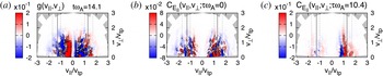
Figure 6. (a) The gyrotropic complementary distribution function
 $g_{p}(v_{\Vert },v_{\bot })$
at a single point in the
$g_{p}(v_{\Vert },v_{\bot })$
at a single point in the
 $\unicode[STIX]{x1D6FD}_{p}=1.0$
turbulent simulation, as well as the correlations (b)
$\unicode[STIX]{x1D6FD}_{p}=1.0$
turbulent simulation, as well as the correlations (b)
 $C_{E_{\Vert }}(\unicode[STIX]{x1D70F}=0)$
and (c)
$C_{E_{\Vert }}(\unicode[STIX]{x1D70F}=0)$
and (c)
 $C_{E_{\Vert }}(\unicode[STIX]{x1D70F}\unicode[STIX]{x1D714}_{A}=10.4)$
at time
$C_{E_{\Vert }}(\unicode[STIX]{x1D70F}\unicode[STIX]{x1D714}_{A}=10.4)$
at time
 $t\unicode[STIX]{x1D714}_{A}=14.1$
. The resonant parallel velocity associated with the maximum proton damping rate is shown as a solid grey vertical line.
$t\unicode[STIX]{x1D714}_{A}=14.1$
. The resonant parallel velocity associated with the maximum proton damping rate is shown as a solid grey vertical line.

Figure 7. Reduced correlations
 $C_{E_{\Vert }}(v_{\Vert })$
for (a)
$C_{E_{\Vert }}(v_{\Vert })$
for (a)
 $v_{\Vert }=0.8v_{\text{tp}}$
and (b)
$v_{\Vert }=0.8v_{\text{tp}}$
and (b)
 $v_{\Vert }=1.3v_{\text{tp}}$
, as well as (c) the velocity integrated
$v_{\Vert }=1.3v_{\text{tp}}$
, as well as (c) the velocity integrated
 $\unicode[STIX]{x2202}w_{p}/\unicode[STIX]{x2202}t$
for correlation intervals ranging from
$\unicode[STIX]{x2202}w_{p}/\unicode[STIX]{x2202}t$
for correlation intervals ranging from
 $0$
(grey) to
$0$
(grey) to
 $20/\unicode[STIX]{x1D714}_{A}$
. Thick black lines indicate the correlation interval selected for figures 6, 8 and 12.
$20/\unicode[STIX]{x1D714}_{A}$
. Thick black lines indicate the correlation interval selected for figures 6, 8 and 12.
Unlike the case for a single KAW presented in figure 3(a), figure 6(a) shows that the structure of the complementary distribution function
 $g_{p}(v_{\Vert },v_{\bot })$
for the strong turbulence simulation has large amplitude fluctuations spread more broadly over velocity space, with the largest amplitude fluctuations occurring at velocities
$g_{p}(v_{\Vert },v_{\bot })$
for the strong turbulence simulation has large amplitude fluctuations spread more broadly over velocity space, with the largest amplitude fluctuations occurring at velocities
 $|v_{\Vert }|\ll v_{\text{tp}}$
. Note also that, for the single KAW case in figure 3(a), the fluctuations in
$|v_{\Vert }|\ll v_{\text{tp}}$
. Note also that, for the single KAW case in figure 3(a), the fluctuations in
 $g_{p}(v_{\Vert },v_{\bot })$
are almost entirely restricted to
$g_{p}(v_{\Vert },v_{\bot })$
are almost entirely restricted to
 $v_{\Vert }>0$
; the reason is because the wave is propagating in only one direction. In the strong turbulence simulation shown in figure 6(a), Alfvénic fluctuations propagate in both directions, thereby leading to significant fluctuations in
$v_{\Vert }>0$
; the reason is because the wave is propagating in only one direction. In the strong turbulence simulation shown in figure 6(a), Alfvénic fluctuations propagate in both directions, thereby leading to significant fluctuations in
 $g_{p}(v_{\Vert },v_{\bot })$
at both
$g_{p}(v_{\Vert },v_{\bot })$
at both
 $v_{\Vert }>0$
and
$v_{\Vert }>0$
and
 $v_{\Vert }<0$
.
$v_{\Vert }<0$
.
Taking the instantaneous correlation
 $C_{E_{\Vert }}$
with
$C_{E_{\Vert }}$
with
 $\unicode[STIX]{x1D70F}=0$
in figure 6(b), which corresponds to the rate of instantaneous energy transfer between the parallel electric field and the ions as a function of gyrotropic velocity space
$\unicode[STIX]{x1D70F}=0$
in figure 6(b), which corresponds to the rate of instantaneous energy transfer between the parallel electric field and the ions as a function of gyrotropic velocity space
 $(v_{\Vert },v_{\bot })$
, we see that the instantaneous energy transfer is also broadly spread over a wide region of velocity space, with significant structure as a function of
$(v_{\Vert },v_{\bot })$
, we see that the instantaneous energy transfer is also broadly spread over a wide region of velocity space, with significant structure as a function of
 $v_{\bot }$
and
$v_{\bot }$
and
 $v_{\Vert }$
. By taking the correlation over the interval
$v_{\Vert }$
. By taking the correlation over the interval
 $\unicode[STIX]{x1D70F}\unicode[STIX]{x1D714}_{A}=10.4$
, equal to a correlation interval
$\unicode[STIX]{x1D70F}\unicode[STIX]{x1D714}_{A}=10.4$
, equal to a correlation interval
 $\unicode[STIX]{x1D70F}=1.67T_{0}$
where
$\unicode[STIX]{x1D70F}=1.67T_{0}$
where
 $T_{0}$
is the period of the largest scale Alfvén waves represented in the simulation, we show in figure 6(c) that the energy transfer is largely restricted to the region near the range of resonant velocities for waves with the highest ion damping rates (within the vertical dashed lines). In addition, the correlated energy transfer is almost entirely a function of
$T_{0}$
is the period of the largest scale Alfvén waves represented in the simulation, we show in figure 6(c) that the energy transfer is largely restricted to the region near the range of resonant velocities for waves with the highest ion damping rates (within the vertical dashed lines). In addition, the correlated energy transfer is almost entirely a function of
 $v_{\Vert }$
, with little significant structure in
$v_{\Vert }$
, with little significant structure in
 $v_{\bot }$
, as expected from kinetic theory for Landau damping. It is remarkable that, even in a strong turbulence simulation, the application of the field–particle correlation technique obtains a velocity-space signature that is qualitatively similar to the case for a single KAW, enabling a straightforward interpretation of the results: the collisionless energy transfer between the parallel electric field and the ions is dominantly a resonant transfer associated with the Landau resonance, a key result of this investigation.
$v_{\bot }$
, as expected from kinetic theory for Landau damping. It is remarkable that, even in a strong turbulence simulation, the application of the field–particle correlation technique obtains a velocity-space signature that is qualitatively similar to the case for a single KAW, enabling a straightforward interpretation of the results: the collisionless energy transfer between the parallel electric field and the ions is dominantly a resonant transfer associated with the Landau resonance, a key result of this investigation.
As with the single KAW case, the selection of the correlation interval
 $\unicode[STIX]{x1D70F}$
is crucial to separating the oscillatory and secular components of the energy transfer. Choosing an appropriate interval is especially challenging in the case of broadband turbulence as there is a spectrum of frequencies associated with the secular energy transfer. To study the impact of the choice of particular values of
$\unicode[STIX]{x1D70F}$
is crucial to separating the oscillatory and secular components of the energy transfer. Choosing an appropriate interval is especially challenging in the case of broadband turbulence as there is a spectrum of frequencies associated with the secular energy transfer. To study the impact of the choice of particular values of
 $\unicode[STIX]{x1D70F}$
, we consider the energy transfer captured by
$\unicode[STIX]{x1D70F}$
, we consider the energy transfer captured by
 $C_{E_{\Vert }}(v_{\Vert })$
, at two values of
$C_{E_{\Vert }}(v_{\Vert })$
, at two values of
 $v_{\Vert }$
, as well as for the velocity integrated correlation for a range of intervals, shown in figure 7.
$v_{\Vert }$
, as well as for the velocity integrated correlation for a range of intervals, shown in figure 7.
As discussed in Howes et al. (Reference Howes, Klein and Li2017) and demonstrated in figure 4 for the single KAW case, if the correlation interval is longer than the wave period of a damping mode, the oscillatory energy transfer will be largely averaged away, leaving mostly the secular component. As there is not a single wave period for turbulent systems, we elect to average the field–particle correlation over an interval much longer than the linear wave period of the most strongly damped mode. As shown in figure 7 with black lines, the selected correlation interval of
 $\unicode[STIX]{x1D70F}\unicode[STIX]{x1D714}_{A}=10.4$
is sufficiently long to remove most of the fluctuations in the energy transfer, leaving a nearly monotonic transfer of energy between the fields and particles.
$\unicode[STIX]{x1D70F}\unicode[STIX]{x1D714}_{A}=10.4$
is sufficiently long to remove most of the fluctuations in the energy transfer, leaving a nearly monotonic transfer of energy between the fields and particles.
With a correlation interval
 $\unicode[STIX]{x1D70F}\unicode[STIX]{x1D714}_{A}=10.4$
selected to isolate the secular energy transfer, we next present the timestack distributions of
$\unicode[STIX]{x1D70F}\unicode[STIX]{x1D714}_{A}=10.4$
selected to isolate the secular energy transfer, we next present the timestack distributions of
 $g_{p}(v_{\Vert },t)$
and the associated reduced field–particle correlations
$g_{p}(v_{\Vert },t)$
and the associated reduced field–particle correlations
 $C_{E_{\Vert }}(v_{\Vert })$
from the same position
$C_{E_{\Vert }}(v_{\Vert })$
from the same position
 $\boldsymbol{r}_{0}$
diagnosed in figure 6. The reduced complementary proton velocity distribution
$\boldsymbol{r}_{0}$
diagnosed in figure 6. The reduced complementary proton velocity distribution
 $g_{p}(v_{\Vert })$
is shown in figure 8(a). As with the gyrotropic plot of
$g_{p}(v_{\Vert })$
is shown in figure 8(a). As with the gyrotropic plot of
 $g_{p}(v_{\Vert },v_{\bot })$
, there is no significant organization of the structure of the distribution
$g_{p}(v_{\Vert },v_{\bot })$
, there is no significant organization of the structure of the distribution
 $g_{p}(v_{\Vert })$
about the preferred parallel resonant velocities of the system, but rather there are large amplitude fluctuations at
$g_{p}(v_{\Vert })$
about the preferred parallel resonant velocities of the system, but rather there are large amplitude fluctuations at
 $|v_{\Vert }|\ll v_{\text{tp}}$
. The instantaneous rate of change of the phase-space energy density as a function of
$|v_{\Vert }|\ll v_{\text{tp}}$
. The instantaneous rate of change of the phase-space energy density as a function of
 $v_{\Vert }$
,
$v_{\Vert }$
,
 $C_{E_{\Vert }}(v_{\Vert },\unicode[STIX]{x1D70F}=0)$
, plotted in figure 8(b), is broadly distributed about the system’s preferred resonant velocities. However, significant oscillatory behaviour in time is retained in the instantaneous energy transfer.
$C_{E_{\Vert }}(v_{\Vert },\unicode[STIX]{x1D70F}=0)$
, plotted in figure 8(b), is broadly distributed about the system’s preferred resonant velocities. However, significant oscillatory behaviour in time is retained in the instantaneous energy transfer.

Figure 8. Timestack plots from the turbulent,
 $\unicode[STIX]{x1D6FD}_{p}=1.0$
simulation, using the same layout as presented in figure 5.
$\unicode[STIX]{x1D6FD}_{p}=1.0$
simulation, using the same layout as presented in figure 5.
The averaged correlation
 $C_{E_{\Vert }}(v_{\Vert },\unicode[STIX]{x1D70F}=10.4)$
is plotted in figure 8(c), which shows clearly that the net energy transfer is localized in the range of the resonant parallel velocities. Again, this velocity-space signature clearly indicates active Landau damping transferring energy to the ions via the parallel electric field of the turbulent fluctuations. Tracking the energy transfer rate at point
$C_{E_{\Vert }}(v_{\Vert },\unicode[STIX]{x1D70F}=10.4)$
is plotted in figure 8(c), which shows clearly that the net energy transfer is localized in the range of the resonant parallel velocities. Again, this velocity-space signature clearly indicates active Landau damping transferring energy to the ions via the parallel electric field of the turbulent fluctuations. Tracking the energy transfer rate at point
 $\boldsymbol{r}_{0}$
, we plot in (d) the velocity-space integrated correlation
$\boldsymbol{r}_{0}$
, we plot in (d) the velocity-space integrated correlation
 $\unicode[STIX]{x2202}w_{p}(\boldsymbol{r}_{0},t)/\unicode[STIX]{x2202}t$
and in (e) the accumulated energy density transfer to the ions
$\unicode[STIX]{x2202}w_{p}(\boldsymbol{r}_{0},t)/\unicode[STIX]{x2202}t$
and in (e) the accumulated energy density transfer to the ions
 $\unicode[STIX]{x0394}w_{p}(\boldsymbol{r}_{0},t)$
. These two metrics show that a net ion energization over time occurs at this position in the simulation.
$\unicode[STIX]{x0394}w_{p}(\boldsymbol{r}_{0},t)$
. These two metrics show that a net ion energization over time occurs at this position in the simulation.
While the resonant signature is not as clean as that seen in simpler Vlasov–Poisson systems, or the single KAW simulation presented earlier in this work, we can quantify the fraction of the energy transferred by resonant particles using the ratio
 $R$
, extended to include the positive and negative resonant velocities. We set
$R$
, extended to include the positive and negative resonant velocities. We set
 $v_{1}=\pm 0.65v_{\text{res},\text{lower}}=0.66v_{\text{tp}}$
and
$v_{1}=\pm 0.65v_{\text{res},\text{lower}}=0.66v_{\text{tp}}$
and
 $v_{2}=\pm 1.35v_{\text{res},\text{upper}}=2.30v_{\text{tp}}$
and plot
$v_{2}=\pm 1.35v_{\text{res},\text{upper}}=2.30v_{\text{tp}}$
and plot
 $R$
in figure 8(f). Over
$R$
in figure 8(f). Over
 $92\,\%$
of the net energy transferred between fields and particles is mediated by the particles in this resonance region. If the energy transfer was equally partitioned based upon the particle density, we would expect only
$92\,\%$
of the net energy transferred between fields and particles is mediated by the particles in this resonance region. If the energy transfer was equally partitioned based upon the particle density, we would expect only
 $35\,\%$
of the net energy transfer to be carried by these particles (vertical grey dot-dashed line). Thus, this analysis shows clearly that a resonant process is governing the net transfer of energy from fields to particles. The key result of this field–particle correlation analysis is that this resonant process, Landau damping, is an effective mechanism for the removal of energy from the turbulent fluctuations in a strongly turbulent, kinetic plasma.
$35\,\%$
of the net energy transfer to be carried by these particles (vertical grey dot-dashed line). Thus, this analysis shows clearly that a resonant process is governing the net transfer of energy from fields to particles. The key result of this field–particle correlation analysis is that this resonant process, Landau damping, is an effective mechanism for the removal of energy from the turbulent fluctuations in a strongly turbulent, kinetic plasma.
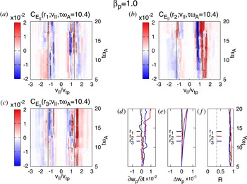
Figure 9. Reduced correlation
 $C_{E_{\Vert }}(v_{\Vert },\unicode[STIX]{x1D70F}\unicode[STIX]{x1D714}_{A}=10.4)$
at three points
$C_{E_{\Vert }}(v_{\Vert },\unicode[STIX]{x1D70F}\unicode[STIX]{x1D714}_{A}=10.4)$
at three points
 $\boldsymbol{r}_{j}$
(a–c) in the
$\boldsymbol{r}_{j}$
(a–c) in the
 $\unicode[STIX]{x1D6FD}_{p}=1.0$
simulation, along with (d) the net energy transfer rate
$\unicode[STIX]{x1D6FD}_{p}=1.0$
simulation, along with (d) the net energy transfer rate
 $\unicode[STIX]{x2202}w_{p}(\boldsymbol{r}_{j},t)/\unicode[STIX]{x2202}t$
and (e) the accumulated energy transfer
$\unicode[STIX]{x2202}w_{p}(\boldsymbol{r}_{j},t)/\unicode[STIX]{x2202}t$
and (e) the accumulated energy transfer
 $\unicode[STIX]{x0394}w_{p}(\boldsymbol{r}_{j},t)$
. Panel (f) shows the fraction of the energy transferred in the region around the preferred resonant velocities,
$\unicode[STIX]{x0394}w_{p}(\boldsymbol{r}_{j},t)$
. Panel (f) shows the fraction of the energy transferred in the region around the preferred resonant velocities,
 $R$
.
$R$
.
6.2 Spatial variation
We next present timestack plots of the reduced correlation
 $C_{E_{\Vert }}(v_{\Vert },\unicode[STIX]{x1D70F}\unicode[STIX]{x1D714}_{A}=10.4)$
at three additional distinct spatial points,
$C_{E_{\Vert }}(v_{\Vert },\unicode[STIX]{x1D70F}\unicode[STIX]{x1D714}_{A}=10.4)$
at three additional distinct spatial points,
 $\boldsymbol{r}_{1}=[6.6,6.6,0]\unicode[STIX]{x1D70C}_{p},~\boldsymbol{r}_{2}=[0,12.6,0]\unicode[STIX]{x1D70C}_{p},$
and
$\boldsymbol{r}_{1}=[6.6,6.6,0]\unicode[STIX]{x1D70C}_{p},~\boldsymbol{r}_{2}=[0,12.6,0]\unicode[STIX]{x1D70C}_{p},$
and
 $\boldsymbol{r}_{3}=[0,6.6,5.5/\unicode[STIX]{x1D716}]\unicode[STIX]{x1D70C}_{p}$
, from the
$\boldsymbol{r}_{3}=[0,6.6,5.5/\unicode[STIX]{x1D716}]\unicode[STIX]{x1D70C}_{p}$
, from the
 $\unicode[STIX]{x1D6FD}_{p}=1.0$
turbulent simulation in figure 9(a–c). The
$\unicode[STIX]{x1D6FD}_{p}=1.0$
turbulent simulation in figure 9(a–c). The
 $v_{\Vert }$
structure of the energy transfer quantitatively differs between the three points but is qualitatively organized by the resonant velocities for all three cases. The net secular energy transfer, calculated by integrating over
$v_{\Vert }$
structure of the energy transfer quantitatively differs between the three points but is qualitatively organized by the resonant velocities for all three cases. The net secular energy transfer, calculated by integrating over
 $v_{\Vert }$
, varies between these points, as shown in figure 9(d) for the net energy density transfer rate
$v_{\Vert }$
, varies between these points, as shown in figure 9(d) for the net energy density transfer rate
 $\unicode[STIX]{x2202}w_{p}(\boldsymbol{r}_{j},t)/\unicode[STIX]{x2202}t$
and (e) for the accumulated energy density transfer to the ions
$\unicode[STIX]{x2202}w_{p}(\boldsymbol{r}_{j},t)/\unicode[STIX]{x2202}t$
and (e) for the accumulated energy density transfer to the ions
 $\unicode[STIX]{x0394}w_{p}(\boldsymbol{r}_{j},t)$
. The spatial variation of the energy transfer to the ions is consistent with previous findings that damping and heating in turbulent systems is not spatially homogeneous but occurs intermittently in space (Wan et al.
Reference Wan, Matthaeus, Karimabadi, Roytershteyn, Shay, Wu, Daughton, Loring and Chapman2012; Karimabadi et al.
Reference Karimabadi, Roytershteyn, Wan, Matthaeus, Daughton, Wu, Shay, Loring, Borovsky and Leonardis2013; TenBarge & Howes Reference TenBarge and Howes2013; Wu et al.
Reference Wu, Perri, Osman, Wan, Matthaeus, Shay, Goldstein, Karimabadi and Chapman2013; Zhdankin et al.
Reference Zhdankin, Uzdensky, Perez and Boldyrev2013, Reference Zhdankin, Uzdensky and Boldyrev2015). Further analysis at other points analysed in the simulation domain (not shown) demonstrates that, although the amplitude and sign of the energy transfer differs from position to position, the energy transfer between the parallel electric field and the ions is dominated by resonant particles, all having values of
$\unicode[STIX]{x0394}w_{p}(\boldsymbol{r}_{j},t)$
. The spatial variation of the energy transfer to the ions is consistent with previous findings that damping and heating in turbulent systems is not spatially homogeneous but occurs intermittently in space (Wan et al.
Reference Wan, Matthaeus, Karimabadi, Roytershteyn, Shay, Wu, Daughton, Loring and Chapman2012; Karimabadi et al.
Reference Karimabadi, Roytershteyn, Wan, Matthaeus, Daughton, Wu, Shay, Loring, Borovsky and Leonardis2013; TenBarge & Howes Reference TenBarge and Howes2013; Wu et al.
Reference Wu, Perri, Osman, Wan, Matthaeus, Shay, Goldstein, Karimabadi and Chapman2013; Zhdankin et al.
Reference Zhdankin, Uzdensky, Perez and Boldyrev2013, Reference Zhdankin, Uzdensky and Boldyrev2015). Further analysis at other points analysed in the simulation domain (not shown) demonstrates that, although the amplitude and sign of the energy transfer differs from position to position, the energy transfer between the parallel electric field and the ions is dominated by resonant particles, all having values of
 $R\approx 0.9$
, as shown in figure 9(f). Therefore, this important result shows definitively that Landau resonant collisionless energy transfer can occur in a spatially non-uniform manner, in contrast to naive expectations of Landau damping based on the plane wave decomposition usually used to derive linear Landau damping. Ongoing work using field–particle correlations will determine whether Landau damping can indeed be responsible for particle energization that is highly intermittent in space, such as that occurring in the vicinity of current sheets, as has been previously suggested (TenBarge & Howes Reference TenBarge and Howes2013; Howes Reference Howes2015, Reference Howes2016).
$R\approx 0.9$
, as shown in figure 9(f). Therefore, this important result shows definitively that Landau resonant collisionless energy transfer can occur in a spatially non-uniform manner, in contrast to naive expectations of Landau damping based on the plane wave decomposition usually used to derive linear Landau damping. Ongoing work using field–particle correlations will determine whether Landau damping can indeed be responsible for particle energization that is highly intermittent in space, such as that occurring in the vicinity of current sheets, as has been previously suggested (TenBarge & Howes Reference TenBarge and Howes2013; Howes Reference Howes2015, Reference Howes2016).
6.3 Variation with plasma
 $\unicode[STIX]{x1D6FD}$

An important test of the application of the field–particle correlation technique to strong plasma turbulence is the dependence of the results on the plasma
 $\unicode[STIX]{x1D6FD}$
. At large scales
$\unicode[STIX]{x1D6FD}$
. At large scales
 $k_{\bot }\unicode[STIX]{x1D70C}_{p}\ll 1$
, the value of the parallel Alfvén wave phase velocity normalized by the Alfvén speed is simply unity,
$k_{\bot }\unicode[STIX]{x1D70C}_{p}\ll 1$
, the value of the parallel Alfvén wave phase velocity normalized by the Alfvén speed is simply unity,
 $\unicode[STIX]{x1D714}/(k_{\Vert }v_{A})=1$
. Normalizing instead to the proton thermal velocity, this relation becomes
$\unicode[STIX]{x1D714}/(k_{\Vert }v_{A})=1$
. Normalizing instead to the proton thermal velocity, this relation becomes
 $\unicode[STIX]{x1D714}/(k_{\Vert }v_{\text{tp}})=v_{A}/v_{\text{tp}}=\unicode[STIX]{x1D6FD}_{p}^{-1/2}$
. Therefore, if the collisionless transfer of energy between the electromagnetic fields and the ions is governed by a resonant mechanism, the field–particle correlation technique will show that the dominant regions of energy transfer in velocity-space shift accordingly as the plasma
$\unicode[STIX]{x1D714}/(k_{\Vert }v_{\text{tp}})=v_{A}/v_{\text{tp}}=\unicode[STIX]{x1D6FD}_{p}^{-1/2}$
. Therefore, if the collisionless transfer of energy between the electromagnetic fields and the ions is governed by a resonant mechanism, the field–particle correlation technique will show that the dominant regions of energy transfer in velocity-space shift accordingly as the plasma
 $\unicode[STIX]{x1D6FD}_{p}$
is changed.
$\unicode[STIX]{x1D6FD}_{p}$
is changed.
We present timestack plots of (a) the reduced complementary distribution function
 $g_{p}(v_{\Vert })=\int \text{d}v_{\bot }g_{p}(v_{\Vert },v_{\bot })$
, (b) the instantaneous phase-space energy density transfer rate
$g_{p}(v_{\Vert })=\int \text{d}v_{\bot }g_{p}(v_{\Vert },v_{\bot })$
, (b) the instantaneous phase-space energy density transfer rate
 $C_{E_{\Vert }}(v_{\Vert },\unicode[STIX]{x1D70F}=0)$
and (c) the time-averaged correlation
$C_{E_{\Vert }}(v_{\Vert },\unicode[STIX]{x1D70F}=0)$
and (c) the time-averaged correlation
 $C_{E_{\Vert }}(v_{\Vert },\unicode[STIX]{x1D70F}\unicode[STIX]{x1D714}_{A}>0)$
for the
$C_{E_{\Vert }}(v_{\Vert },\unicode[STIX]{x1D70F}\unicode[STIX]{x1D714}_{A}>0)$
for the
 $\unicode[STIX]{x1D6FD}_{p}=0.3$
simulation in figure 10 and for the
$\unicode[STIX]{x1D6FD}_{p}=0.3$
simulation in figure 10 and for the
 $\unicode[STIX]{x1D6FD}_{p}=3.0$
simulation in figure 11. As expected from the scaling
$\unicode[STIX]{x1D6FD}_{p}=3.0$
simulation in figure 11. As expected from the scaling
 $\unicode[STIX]{x1D714}/(k_{\Vert }v_{\text{tp}})\propto \unicode[STIX]{x1D6FD}_{p}^{-1/2}$
, illustrated in figure 1, the preferred resonant velocities are shifted to higher
$\unicode[STIX]{x1D714}/(k_{\Vert }v_{\text{tp}})\propto \unicode[STIX]{x1D6FD}_{p}^{-1/2}$
, illustrated in figure 1, the preferred resonant velocities are shifted to higher
 $v_{\Vert }$
for lower
$v_{\Vert }$
for lower
 $\unicode[STIX]{x1D6FD}_{p}$
, and lower
$\unicode[STIX]{x1D6FD}_{p}$
, and lower
 $v_{\Vert }$
for higher
$v_{\Vert }$
for higher
 $\unicode[STIX]{x1D6FD}_{p}$
, specifically
$\unicode[STIX]{x1D6FD}_{p}$
, specifically
 $\unicode[STIX]{x1D714}/k_{\Vert }=2.00v_{\text{tp}}$
for
$\unicode[STIX]{x1D714}/k_{\Vert }=2.00v_{\text{tp}}$
for
 $\unicode[STIX]{x1D6FD}_{p}=0.3$
and
$\unicode[STIX]{x1D6FD}_{p}=0.3$
and
 $\unicode[STIX]{x1D714}/k_{\Vert }=0.626v_{\text{tp}}$
for
$\unicode[STIX]{x1D714}/k_{\Vert }=0.626v_{\text{tp}}$
for
 $\unicode[STIX]{x1D6FD}_{p}=3.0$
. We choose correlation intervals,
$\unicode[STIX]{x1D6FD}_{p}=3.0$
. We choose correlation intervals,
 $\unicode[STIX]{x1D70F}\unicode[STIX]{x1D714}_{A}=16.1$
and
$\unicode[STIX]{x1D70F}\unicode[STIX]{x1D714}_{A}=16.1$
and
 $9.70$
for the
$9.70$
for the
 $\unicode[STIX]{x1D6FD}_{p}=0.3$
and
$\unicode[STIX]{x1D6FD}_{p}=0.3$
and
 $3.0$
simulations to remove the oscillatory component of the energy transfer. In (d,e), the net secular energy density transfer rate
$3.0$
simulations to remove the oscillatory component of the energy transfer. In (d,e), the net secular energy density transfer rate
 $\unicode[STIX]{x2202}w_{p}(\boldsymbol{r}_{j},t)/\unicode[STIX]{x2202}t$
and the accumulated energy density transfer
$\unicode[STIX]{x2202}w_{p}(\boldsymbol{r}_{j},t)/\unicode[STIX]{x2202}t$
and the accumulated energy density transfer
 $\unicode[STIX]{x0394}w_{p}(\boldsymbol{r}_{j},t)$
is plotted, showing a net transfer of energy to the ions from the electric field.
$\unicode[STIX]{x0394}w_{p}(\boldsymbol{r}_{j},t)$
is plotted, showing a net transfer of energy to the ions from the electric field.
The fraction of energy transferred by particles with parallel velocities near the resonant velocities,
 $R$
, is large for both simulations. As with the
$R$
, is large for both simulations. As with the
 $\unicode[STIX]{x1D6FD}_{p}=1.0$
turbulent simulation, we select
$\unicode[STIX]{x1D6FD}_{p}=1.0$
turbulent simulation, we select
 $|v_{1}|=0.65v_{\text{res},\text{lower}}$
and
$|v_{1}|=0.65v_{\text{res},\text{lower}}$
and
 $|v_{2}|=1.35v_{\text{res},\text{upper}}$
, where
$|v_{2}|=1.35v_{\text{res},\text{upper}}$
, where
 $v_{\text{res},\text{lower}}$
and
$v_{\text{res},\text{lower}}$
and
 $v_{\text{res},\text{upper}}$
are the resonant velocities associated with the KAW wave modes having proton damping rates equal to
$v_{\text{res},\text{upper}}$
are the resonant velocities associated with the KAW wave modes having proton damping rates equal to
 $1/e$
of the peak proton damping rate. This selection results in
$1/e$
of the peak proton damping rate. This selection results in
 $|v_{1}|=1.188(0.378)v_{\text{tp}}$
and
$|v_{1}|=1.188(0.378)v_{\text{tp}}$
and
 $|v_{2}|=3.193(1.330)v_{\text{tp}}$
for the
$|v_{2}|=3.193(1.330)v_{\text{tp}}$
for the
 $\unicode[STIX]{x1D6FD}_{p}=0.3(3.0)$
simulation, and yields
$\unicode[STIX]{x1D6FD}_{p}=0.3(3.0)$
simulation, and yields
 $R=0.75(0.7)$
, shown in (f). If the energy transfer was equally partitioned based upon velocity-space density, these particles would only be responsible for
$R=0.75(0.7)$
, shown in (f). If the energy transfer was equally partitioned based upon velocity-space density, these particles would only be responsible for
 $9\,\%$
and
$9\,\%$
and
 $53\,\%$
of the energy transfer respectively. Thus, for all examined values of
$53\,\%$
of the energy transfer respectively. Thus, for all examined values of
 $\unicode[STIX]{x1D6FD}_{p}$
, the phase-space energy transfer is largely consistent with the linear predictions for resonant Landau damping. We note that we have restricted this work to
$\unicode[STIX]{x1D6FD}_{p}$
, the phase-space energy transfer is largely consistent with the linear predictions for resonant Landau damping. We note that we have restricted this work to
 $\unicode[STIX]{x1D6FD}_{p}$
near unity to model typical 1 AU solar wind turbulence, restricting
$\unicode[STIX]{x1D6FD}_{p}$
near unity to model typical 1 AU solar wind turbulence, restricting
 $v_{\Vert ,\text{res}}\sim v_{\text{tp}}$
. Future work is underway to study the effects of significant departures from
$v_{\Vert ,\text{res}}\sim v_{\text{tp}}$
. Future work is underway to study the effects of significant departures from
 $\unicode[STIX]{x1D6FD}_{p}=1$
on the secular transfer of energy, as both magnetically and thermally dominated plasmas are relevant in different space and astrophysical contexts.
$\unicode[STIX]{x1D6FD}_{p}=1$
on the secular transfer of energy, as both magnetically and thermally dominated plasmas are relevant in different space and astrophysical contexts.

Figure 10. Timestack plots from the turbulent,
 $\unicode[STIX]{x1D6FD}_{p}=0.3$
simulation, using the same layout as presented in figure 5.
$\unicode[STIX]{x1D6FD}_{p}=0.3$
simulation, using the same layout as presented in figure 5.

Figure 11. Timestack plots from the turbulent,
 $\unicode[STIX]{x1D6FD}_{p}=3.0$
simulation, using the same layout as presented in figure 5.
$\unicode[STIX]{x1D6FD}_{p}=3.0$
simulation, using the same layout as presented in figure 5.
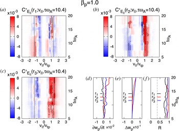
Figure 12. Reduced correlation
 $C_{E_{\Vert }}^{\prime }(v_{\Vert },\unicode[STIX]{x1D70F}\unicode[STIX]{x1D714}_{A}=10.4)$
and integrated quantities at the same three points in the
$C_{E_{\Vert }}^{\prime }(v_{\Vert },\unicode[STIX]{x1D70F}\unicode[STIX]{x1D714}_{A}=10.4)$
and integrated quantities at the same three points in the
 $\unicode[STIX]{x1D6FD}_{p}=1.0$
simulation shown in figure 9.
$\unicode[STIX]{x1D6FD}_{p}=1.0$
simulation shown in figure 9.
6.4 Alternative field–particle correlation
$C_{E_{\Vert }}^{\prime }$

As discussed in § 2, limitations of spacecraft data make velocity gradients
 $\unicode[STIX]{x2202}f_{s}(\boldsymbol{v})/\unicode[STIX]{x2202}v_{\Vert }$
noisy and potentially unreliable. To alleviate this problem, an alternative correlation,
$\unicode[STIX]{x2202}f_{s}(\boldsymbol{v})/\unicode[STIX]{x2202}v_{\Vert }$
noisy and potentially unreliable. To alleviate this problem, an alternative correlation,
 $C_{E_{\Vert }}^{\prime }$
, was introduced in (2.10). This alternative correlation is calculated over the same correlation interval
$C_{E_{\Vert }}^{\prime }$
, was introduced in (2.10). This alternative correlation is calculated over the same correlation interval
 $\unicode[STIX]{x1D70F}$
and at the same three spatial points
$\unicode[STIX]{x1D70F}$
and at the same three spatial points
 $\boldsymbol{r}_{j}$
used for figure 9 and is shown in figure 12(a–c). As has been previously noted for application of this technique to electrostatic systems, the resonant signature – that is, the change in sign of the phase-space energy transfer rate across a preferred velocity – is not present in the structure of
$\boldsymbol{r}_{j}$
used for figure 9 and is shown in figure 12(a–c). As has been previously noted for application of this technique to electrostatic systems, the resonant signature – that is, the change in sign of the phase-space energy transfer rate across a preferred velocity – is not present in the structure of
 $C_{E_{\Vert }}^{\prime }$
. Nevertheless, a calculation of the resonant fraction
$C_{E_{\Vert }}^{\prime }$
. Nevertheless, a calculation of the resonant fraction
 $R$
replacing
$R$
replacing
 $C_{E_{\Vert }}$
with
$C_{E_{\Vert }}$
with
 $C_{E_{\Vert }}^{\prime }$
, shows that the amplitude of the alternative correlation remains significantly enhanced in the resonant particle region. Comparison of the (d) net energy density transfer rate
$C_{E_{\Vert }}^{\prime }$
, shows that the amplitude of the alternative correlation remains significantly enhanced in the resonant particle region. Comparison of the (d) net energy density transfer rate
 $\unicode[STIX]{x2202}w_{p}(\boldsymbol{r}_{j},t)/\unicode[STIX]{x2202}t$
and (e) the accumulated energy density transfer to the ions
$\unicode[STIX]{x2202}w_{p}(\boldsymbol{r}_{j},t)/\unicode[STIX]{x2202}t$
and (e) the accumulated energy density transfer to the ions
 $\unicode[STIX]{x0394}w_{p}(\boldsymbol{r}_{j},t)$
for the standard correlation
$\unicode[STIX]{x0394}w_{p}(\boldsymbol{r}_{j},t)$
for the standard correlation
 $C_{E_{\Vert }}$
in figure 9 and for the alternative correlation
$C_{E_{\Vert }}$
in figure 9 and for the alternative correlation
 $C_{E_{\Vert }}^{\prime }$
in figure 12 shows that the two forms of the correlation yield identical results. This must hold, since the integrated quantities are related by an integration by parts in velocity (Howes et al.
Reference Howes, Klein and Li2017), both simply tracking the same averaged
$C_{E_{\Vert }}^{\prime }$
in figure 12 shows that the two forms of the correlation yield identical results. This must hold, since the integrated quantities are related by an integration by parts in velocity (Howes et al.
Reference Howes, Klein and Li2017), both simply tracking the same averaged
 $j_{p\Vert }E_{\Vert }$
energy transfer rate. The agreement serves as a check that both analysis methods are being applied correctly.
$j_{p\Vert }E_{\Vert }$
energy transfer rate. The agreement serves as a check that both analysis methods are being applied correctly.
7 Conclusions and future work
Here we have applied the field–particle correlation technique (Klein & Howes Reference Klein and Howes2016; Howes et al. Reference Howes, Klein and Li2017) to explore the ion energization in gyrokinetic simulations of strong plasma turbulence. The results definitively show that Landau damping persists as an effective physical mechanism for ion energization in strong plasma turbulence, contradicting recent suggestions that Landau damping may become ineffective in the highly nonlinear environment of strong turbulence (Plunk Reference Plunk2013; Schekochihin et al. Reference Schekochihin, Parker, Highcock, Dellar, Dorland and Hammett2016). Furthermore, it is shown directly that the ion energization resulting from the Landau damping of turbulent electromagnetic fluctuations is spatially non-uniform, in contrast to naive expectations that Landau damping leads to spatially uniform energization, likely arising from the plane wave decomposition typically used to derive linear Landau damping. Further work using field–particle correlations will address whether Landau damping can effectively lead to the spatially intermittent plasma heating in the vicinity of current sheets found in plasma turbulence simulations (Wan et al. Reference Wan, Matthaeus, Karimabadi, Roytershteyn, Shay, Wu, Daughton, Loring and Chapman2012; Karimabadi et al. Reference Karimabadi, Roytershteyn, Wan, Matthaeus, Daughton, Wu, Shay, Loring, Borovsky and Leonardis2013; TenBarge & Howes Reference TenBarge and Howes2013; Wu et al. Reference Wu, Perri, Osman, Wan, Matthaeus, Shay, Goldstein, Karimabadi and Chapman2013; Zhdankin et al. Reference Zhdankin, Uzdensky, Perez and Boldyrev2013) and inferred from solar wind observations (Osman et al. Reference Osman, Matthaeus, Greco and Servidio2011, Reference Osman, Matthaeus, Wan and Rappazzo2012; Perri et al. Reference Perri, Goldstein, Dorelli and Sahraoui2012; Wang et al. Reference Wang, Tu, He, Marsch and Wang2013; Wu et al. Reference Wu, Perri, Osman, Wan, Matthaeus, Shay, Goldstein, Karimabadi and Chapman2013; Osman et al. Reference Osman, Kiyani, Chapman and Hnat2014a ).
Simulations with a wider range of plasma parameters than considered in this work, especially more significant variations in
 $\unicode[STIX]{x1D6FD}_{p}$
, will be useful in further testing the applicability of this correlation to a wide range of solar wind parameters. This work only focuses on a single class of dissipation mechanisms which satisfy the Landau (
$\unicode[STIX]{x1D6FD}_{p}$
, will be useful in further testing the applicability of this correlation to a wide range of solar wind parameters. This work only focuses on a single class of dissipation mechanisms which satisfy the Landau (
 $n=0$
) resonance. Future work will focus on characterizing the velocity-space structure of field–particle correlations due to other damping mechanisms, including
$n=0$
) resonance. Future work will focus on characterizing the velocity-space structure of field–particle correlations due to other damping mechanisms, including
 $n\neq 0$
cyclotron damping, stochastic ion heating by low-frequency Alfvénic turbulence, and energization via magnetic reconnection. Comparing correlations constructed using different components of the electric field and comparing where in velocity and configuration space energy transfer occurs will enable the determination of the relative contribution of proposed mechanisms to the dissipation of turbulence.
$n\neq 0$
cyclotron damping, stochastic ion heating by low-frequency Alfvénic turbulence, and energization via magnetic reconnection. Comparing correlations constructed using different components of the electric field and comparing where in velocity and configuration space energy transfer occurs will enable the determination of the relative contribution of proposed mechanisms to the dissipation of turbulence.
This work demonstrates that field–particle correlations can be usefully applied to data from single-point measurements of turbulent space plasmas. Application of this technique to current and proposed missions, such as DSCOVR, Magnetospheric Multiscale (MMS) (Burch et al.
Reference Burch, Moore, Torbert and Giles2016), Parker Solar Probe (Fox et al.
Reference Fox, Velli, Bale, Decker, Driesman, Howard, Kasper, Kinnison, Kusterer and Lario2015) and Turbulence Heating ObserveR (THOR) (Vaivads et al.
Reference Vaivads, Retinò, Soucek, Khotyaintsev, Valentini, Escoubet, Alexandrova, André, Bale and Balikhin2016) may enable the definitive identification of the mechanisms which dissipate turbulence and heat the solar wind as it expands through the heliosphere. The alternative correlation
 $C_{E_{\Vert }}^{\prime }$
, which is easier to employ on noisy and lower velocity-space resolution solar wind observations, is able to isolate the regions in velocity space where the energy transfer is occurring.
$C_{E_{\Vert }}^{\prime }$
, which is easier to employ on noisy and lower velocity-space resolution solar wind observations, is able to isolate the regions in velocity space where the energy transfer is occurring.
Acknowledgements
The authors would like to thank B. Chandran, B. Dorland and J. Kasper for helpful discussions during the execution of this project. This work was supported by NASA grant HSR NNX16AM23G, NSF grant CAREER AGS-1054061, NSF SHINE award AGS-1622306, and DOE grant DE-SC0014599. This work used the Extreme Science and Engineering Discovery Environment (XSEDE), which is supported by National Science Foundation grant no. ACI-1053575.


