


Introduction
Genomic selection refers to the use of genome wide and dense markers for the prediction of breeding values (BV) and subsequent selection of individuals (Meuwissen et al., Reference Meuwissen, Hayes and Goddard2001). Results from simulations and from real validation studies revealed that the accuracy of predicted BV of individuals without own records or without progeny records can be remarkably high (Meuwissen et al., Reference Meuwissen, Hayes and Goddard2001; Calus et al., Reference Calus, Meuwissen, de Roos and Veerkamp2008; Luan et al., Reference Luan, Woolliams, Lien, Kent, Svendsen and Meuwissen2009; Habier et al., Reference Habier, Tetens, Seefried, Lichtner and Thaller2010; Hayes et al., Reference Hayes, Bowman, Chamberlain and Goddard2009), which offers the opportunity to accurately select individuals at an early stage of their life as parents of the next generation. This technique has become a standard tool in dairy cattle breeding (Hayes et al., Reference Hayes, Bowman, Chamberlain and Goddard2009), and its implementation in other livestock species is foreseen, e.g. in poultry breeding (Wolc et al., Reference Wolc, Stricker, Arango, Settar, Fulton, O'Sullivan, Preisinger, Habier, Fernando, Garrick, Lamont and Deckers2011), in pig breeding, and also in plant breeding (Piepho, Reference Piepho2009; Heffner et al., Reference Heffner, Sorrells and Jannink2009).
The core of genomic selection is the prediction of BV from massive marker data. Most influential methods were already proposed by Meuwissen et al. (Reference Meuwissen, Hayes and Goddard2001). These are genomic best linear unbiased prediction (G-BLUP), BayesA and BayesB, which differ in their assumptions about the distribution of marker effects. G-BLUP assumes a normal distribution of marker effects, whereas BayesA assumes a more heavy tailed Student t-distribution (Gianola et al., Reference Gianola, de los Campos, Hill, Manfredi and Fernando2009). Since the Student t-distribution approximates the normal distribution when the degree of freedom v increases, G-BLUP can be considered as a limiting case of BayesA. Although these methods perform well in simulation studies and applications, many markers are not needed to capture the effects of quantitative trait loci (QTLs) because they are either redundant or not in linkage disequilibrium (LD) with a QTL. This is accounted for by BayesB, which assumes that marker effects come from a Student t-distribution with a certain probability and take the value 0 otherwise. A marker effect comes from the Student t-distribution if the marker is needed to capture a QTL effect. BayesB contains BayesA as the special case where the prior probability of a marker to be needed equals one. An alternative is the stochastic search variable selection (SSVS) model (George & McCulloch, Reference George and McCulloch1993) that was introduced to QTL mapping by Yi et al. (Reference Yi, George and Allison2003) and was applied by Meuwissen (Reference Meuwissen2009) to genomic selection. It assumes that effects of single nucleotide polymorphisms (SNPs) come from a mixture of two normal distributions with different variances, and SNPs with negligible effects come from the distribution with little variance. Bayesian SSVS is similar, but assumes prior distributions for the variances of SNP effects. As a consequence, SNP effects are from a mixture of two Student t-distributions with different variances. Bayesian SSVS is also known as BayesC (Verbyla et al., Reference Verbyla, Hayes, Bowman and Goddard2009, Reference Verbyla, Bowman, Hayes and Goddard2010). It contains BayesB as the limiting case, in which the variance of one mixing distribution approaches zero. Further Bayesian models that have been proposed are the Bayesian Lasso that assumes Laplace priors (Park & Casella, Reference Park and Casella2008; Legarra et al., Reference Legarra, Robert-Granié, Croiseau, Guillaume and Fritz2011), and a Bayesian model that uses identity by descent (IBD) probabilities (Meuwissen & Goddard, Reference Meuwissen and Goddard2004). However, Calus et al. (Reference Calus, Meuwissen, de Roos and Veerkamp2008) found that a marker effect–based model that does not make use of IBD probabilities provides similar accuracies for high–density marker panels.
Nearly all published models only include additive effects (Calus, Reference Calus2010) and little has been done to generalize these models for the prediction of genomic BV to explicitly account for dominance. One reason is probably that estimated BV or deregressed BV obtained from routine evaluations (Garrick et al., Reference Garrick, Taylor and Fernando2009) are used as observations in most applications of genomic selection, so dominance deviations of individuals are absent in the data. However, if individual phenotypes are available, the inclusion of dominance effects could not only increase the accuracy of genomic selection, but predicted dominance effects could also be used to find mating pairs with good combining abilities by recovering inbreeding depression and utilizing possible overdominance. Toro & Varona (Reference Toro and Varona2010) demonstrated that the inclusion of dominance into Bayesian models can indeed increase the accuracy of genomic selection. They assumed independent additive and dominance effects which were in accordance with their simulation protocol. Reproducing kernel Hilbert space regression (RKHS regression) is proposed as an alternative method for the estimation of genotypic values (GV), especially if non-additive effects such as dominance or epistasis are included in the phenotypes (Gianola et al., Reference Gianola, Fernando and Stella2006). It assumes that for each pair of genotypes, the covariance of its GV is defined by a covariance function (de los Campos et al., Reference de los Campos, Gianola and Rosa2009). The covariance function is the reproducing kernel of a Hilbert space. RKHS regression yields an estimate of the function g that maps genotypes to GV. This estimate is optimal in a well–defined sense among all functions that belong to the Hilbert space (Gianola & van Kaam, Reference Gianola and de los Campos2008). RKHS regression does not make assumptions about the mechanism that makes GV random since any symmetric and finitely positive-semidefinite function K is the reproducing kernel of a Hilbert Space (Shawe-Taylor & Cristianini, Reference Shawe-Taylor and Cristianini2004).
The aim of this paper is to introduce Bayesian linear regression models for genomic evaluation of quantitative traits that account for dominance effects of QTLs. These models are generalizations of Bayesian SSVS that includes only additive effects. The proposed models differ in the way the dependency between additive effects, dominance effects and allele frequencies is modelled. Plausible informative priors are chosen which are in agreement with the genetic architectures of quantitative traits suggested in the literature. We call these generalizations the BayesD models, where D stands for dominance. The paper is organized as follows. We start with a brief literature review on the dependencies between additive effects, dominance effects and allele frequencies in real populations and discuss how Bayesian models could account for these dependencies. Statistical models that realistically account for these dependencies are defined thereafter. The joint posterior distribution of unknown model parameters is given and used to derive a Markov chain for the prediction of these parameters. Moments of the random effects are derived and are used for the calculation of the hyper-parameters. We also demonstrate that kernels for RKHS regression can be derived from the assumptions of our models. The resulting RKHS estimate is the BLUP for the underlying Bayesian model. The proposed methods are applied to a simulated population. The models are compared with respect to their ability to predict dominance deviations, GV and BV.
Theory
Possibilities to model the genetics of dominance
Since the aim of this paper is to account for dominance in genomic evaluations of quantitative traits, we present different possibilities to model the joint distribution of additive and dominance effects of the markers and show how these models are able to account for the genetic architectures that are suggested in the literature. The mathematical definitions of our models are given in the next section. Note that the proofs of all numbered equations can be found in the electronic appendix. Table 1 summarizes symbols used in this paper.
Table 1. Table of symbols

Consider biallelic QTLs with alleles 0 and 1. In this section, a j and d j denote the additive and dominance effect of QTL j. The 1-allele has frequency p j and the 0-allele has frequency q j=1−p j. The three possible genotypes 00, 01 and 11 have GV 0, a j+d j and 2 a j. Dominance effects can cause inbreeding depression. Inbreeding depression ![]() of a trait is the expected decrease of the phenotypic value when the inbreeding coefficient increases from 0 to 1.
of a trait is the expected decrease of the phenotypic value when the inbreeding coefficient increases from 0 to 1. ![]() >0 requires that the expectation of dominance effects is positive, provided that allelic effects are assumed to be random realisations from some distribution. This means that the effect of the heterozygous genotype is usually above the average effect of the two homozygous genotypes. Analogously, for a trait with outbreeding depression we have
>0 requires that the expectation of dominance effects is positive, provided that allelic effects are assumed to be random realisations from some distribution. This means that the effect of the heterozygous genotype is usually above the average effect of the two homozygous genotypes. Analogously, for a trait with outbreeding depression we have ![]() <0 and the expectation of dominance effects is negative. Dominance effects also cause dominance variance. Dominance variances of up to 50% of the additive variance have been reported for traits in dairy cattle (van Tassell et al., Reference van Tassell, Misztal and Varona2000). Substantially larger dominance variances are unlikely to occur due to the U-shaped distribution of allele frequencies (Hill et al., Reference Hill, Goddard and Visscher2008). Dominance variances have also been estimated for some traits in beef cattle (Duangjinda et al., Reference Duangjinda, Bertrand, Misztal and Druet2001) and pigs (Serenius et al., Reference Serenius, Stalder and Puonti2006). In general, estimates of dominance variance must be interpreted with caution because they could be confounded e.g. by maternal effects or environmental covariance of full sibs. Moreover, an accurate estimation of dominance variance requires at least 20 times as much data as the estimation of additive variance (Misztal, Reference Misztal1997).
<0 and the expectation of dominance effects is negative. Dominance effects also cause dominance variance. Dominance variances of up to 50% of the additive variance have been reported for traits in dairy cattle (van Tassell et al., Reference van Tassell, Misztal and Varona2000). Substantially larger dominance variances are unlikely to occur due to the U-shaped distribution of allele frequencies (Hill et al., Reference Hill, Goddard and Visscher2008). Dominance variances have also been estimated for some traits in beef cattle (Duangjinda et al., Reference Duangjinda, Bertrand, Misztal and Druet2001) and pigs (Serenius et al., Reference Serenius, Stalder and Puonti2006). In general, estimates of dominance variance must be interpreted with caution because they could be confounded e.g. by maternal effects or environmental covariance of full sibs. Moreover, an accurate estimation of dominance variance requires at least 20 times as much data as the estimation of additive variance (Misztal, Reference Misztal1997).
Figure 1 gives an overview of different possibilities to model the joint distribution of additive effects and dominance effects. The figure shows samples drawn from the proposed joint prior distribution of additive and dominance effects of markers with allele frequency q j=p j=0·5 for different scenarios, where additive effects are assumed to be Student t-distributed with v=2·5 degrees of freedom. Note that the models presented in the next section are more general than this illustrative example.

Fig. 1. Samples drawn from the joint prior distribution of additive and dominance effects of markers with allele frequency qj =pj =0·5, where additive effects are Student t-distributed with v=2·5 degrees of freedom. The distribution specifications of BayesD1–BayesD3 are given in Section 2(ii).
The simplest possibility is to assume independence of additive and dominance effects, where dominance effects have the same distribution as additive effects. It can be seen in Fig. 1 that this prior assumes that for QTL with large dominance effect the additive effect is likely small in magnitude. This is because the t-distribution is heavy tailed, so it allows ‘large’ effects to occur. But large effects are rare events, so under independence, the probability is small that for a large dominance effect, the additive effect is also large. Thus, dominance is mainly due to overdominant alleles. But this is out of line with standard genetics theory (Kacser & Burns, Reference Kacser and Burns1981; Charlesworth & Willis, Reference Charlesworth and Willis2009) because theory predicts that recessive deleterious alleles rather than overdominant alleles are the primary cause of inbreeding depression. This model is therefore not further considered.
A second possibility (BayesD1) is to assume that the joint distribution of additive and dominance effects is elliptical with Student t-distributed margins. Roughly speaking, this model assumes that additive and dominance effects of a QTL are of the same magnitude. Figure 1 shows that overdominance is quite common under this assumption. The importance of overdominance cannot yet be accurately quantified (Charlesworth & Willis, Reference Charlesworth and Willis2009), so this model may be appropriate for populations in which many overdominant QTLs are expected to exist. For most applications, however, the prior possibly allows for too much overdominance.
Therefore, we consider as a third possibility (BayesD2) the case that absolute additive effects and dominance coefficients are independent. The dominance coefficient ![]() of a QTL is the ratio between the dominance effect and the absolute additive effect. If δj>1 or δj<−1 then the QTL is overdominant (or underdominant). If δj=1 or δj=−1 then the QTL is dominant or recessive. For δj=0, the QTL is completely additive and a QTL with −1<δj<0 or 0<δj<1 shows incomplete dominance or recessivity. As demonstrated in Fig. 1, the model is able to make the prior assumption that the probability is small that a dominance effect is much larger in magnitude than the additive effect, so overdominance is a rare but not negligible event. This is in accordance with Bennewitz & Meuwissen (Reference Bennewitz and Meuwissen2010) who used results from QTL experiments and found that dominance coefficients were normally distributed with small but positive mean. Here, we also assume a normal distribution for the dominance coefficient.
of a QTL is the ratio between the dominance effect and the absolute additive effect. If δj>1 or δj<−1 then the QTL is overdominant (or underdominant). If δj=1 or δj=−1 then the QTL is dominant or recessive. For δj=0, the QTL is completely additive and a QTL with −1<δj<0 or 0<δj<1 shows incomplete dominance or recessivity. As demonstrated in Fig. 1, the model is able to make the prior assumption that the probability is small that a dominance effect is much larger in magnitude than the additive effect, so overdominance is a rare but not negligible event. This is in accordance with Bennewitz & Meuwissen (Reference Bennewitz and Meuwissen2010) who used results from QTL experiments and found that dominance coefficients were normally distributed with small but positive mean. Here, we also assume a normal distribution for the dominance coefficient.
Caballero & Keightley (Reference Caballero and Keightley1994) showed that the dominance effect depends on the additive effect such that QTLs with large absolute additive effect likely have large dominance coefficients. Moreover, they concluded tentatively that mutations of small effect show highly variable degrees of dominance with an average dominance coefficient close to zero. Deleterious alleles with large effect are usually close to recessivity due to the hyperbolic relationship between enzyme activity and flux (Kacser & Burns, Reference Kacser and Burns1981). The prior distribution of BayesD2 cannot account for this. Therefore, we consider as a fourth possibility (BayesD3) the case that markers with large absolute additive effects tend to be associated with large dominance coefficients. That is, for additive effects of markers that are small in magnitude, the average dominance coefficient is close to 0, and for additive effects of markers that are large in magnitude the average dominance coefficient is close to 1. This is also in accordance with García-Dorado et al. (Reference García-Dorado, López-Fanjul and Caballero1999), who suggested an average dominance coefficient of 0·8 for non-severe deleterious mutations and of 0·94–0·98 for new lethal mutants.
In addition to the dependency between dominance effects and absolute additive effects, the dependency between the allele frequencies and the signs of the allelic effects could also be considered. They are dependent because selection has likely shifted allele frequencies away from values for which the expected allele-frequency change per one generation of selection is high. From this argument, a characterization of the dependency can be derived as follows: since selection for (or against) a recessive allele is inefficient if its frequency is low (Falconer & Mackay, Reference Falconer and Mackay1996; Fig. 2.2), recessive alleles likely have low frequencies. Recessiveness of the 1-allele implies that d j<0 if a j>0 and d j>0 if a j<0. Since p j<0·5 is likely to hold, we have sign(a j)=−sign((q j−p j)d j) in both cases. Now consider selection for (or against) a dominant allele. If the 1-allele is dominant, then the other allele is recessive. From the above argument it follows that the other allele likely has a low frequency (q j<0·5). It follows that p j>0·5. Thus, dominant alleles likely have high frequencies. Dominance of the 1-allele implies that d j>0 if a j>0 and d j<0 if a j<0. Since p j>0·5 is likely to hold, we have again sign(a j)=−sign((q j−p j)d j) with high probability. The models BayesD2 and BayesD3 account for this. Alternatively, the equation could be derived from the contribution 2p jq j(a j+(q j−p j)d j)2 of the QTL to the additive variance because it is unlikely that a QTL has a frequency p j for which the contribution of the QTL to the additive variance is large. The contribution is small if a j≈−(q j−p j)d j. This also shows that sign(a j)=sign(−(q j−p j)d j) likely holds for the majority of the alleles. Wellmann & Bennewitz (Reference Wellmann and Bennewitz2011) obtained plausible estimates for parameters of the joint distribution of additive effects and dominance effects for the trait productive life (PL) in dairy cattle only if the model accounts for this. From this argument it also follows that alleles with large effect are not likely to have intermediate frequencies, except for overdominant alleles (Falconer & Mackay, Reference Falconer and Mackay1996; p. 27ff.) and some pleiotropic alleles (e.g. DGAT1 in Holstein cattle, see Grisart et al., Reference Grisart, Farnir, Karim, Cambisano, Kim, Kvasz, Mni, Simon, Frère, Coppieters and Georges2004).
The linear regression model
In this section, the general regression model and various submodels are defined. The submodels differ in the joint prior distributions of the additive and dominance effects of the markers as motivated in the previous section. We consider a linear model of the form
where the vector y consists of n observations, β is a vector of fixed effects and would usually include the intercept of the model. The matrix X has full column rank. The vector u~![]() p(0, Σ) is normally distributed and independent from the marker effects with covariance matrix Σ and Z is a known n×p matrix. The vector
p(0, Σ) is normally distributed and independent from the marker effects with covariance matrix Σ and Z is a known n×p matrix. The vector ![]() contains the additive effects of the markers and
contains the additive effects of the markers and ![]() consists of the dominance effects of the markers, where M is the number of markers. The errors E 1, …, E n are independent and normally distributed with variance σ2, i.e. E|σ2~
consists of the dominance effects of the markers, where M is the number of markers. The errors E 1, …, E n are independent and normally distributed with variance σ2, i.e. E|σ2~![]() n(0, σ2I).
n(0, σ2I).
Additive effects and dominance effects of the markers are random variables. Randomness of allelic effects is most easily understood by imagining that the population is a random sample from all hypothetical populations to which the method could be applied, and the trait is randomly chosen among all traits with similar genetic architecture that could be analysed. That is, for each hypothetical population the effect of a marker at a particular position in the genome is a random realization from some distribution. We assume biallelic markers with alleles 0 and 1. Take ![]() to be the effect of marker j. We have
to be the effect of marker j. We have ![]() , if dominance effects are included in the model and
, if dominance effects are included in the model and ![]() otherwise. It is assumed that the distribution of
otherwise. It is assumed that the distribution of ![]() is a mixture of two distributions that differ only by a scaling factor ε, so conditionally on a Bernoulli distributed indicator variable γj~
is a mixture of two distributions that differ only by a scaling factor ε, so conditionally on a Bernoulli distributed indicator variable γj~![]() (1, p LD) we can write
(1, p LD) we can write
where the parameter 0⩽ε≪1 is chosen small and the distribution ![]() is specified below. Thus, if γj=1, then the marker effect comes from the distribution with large variance. This occurs with probability p LD=E(γj). Markers j with γj=1 are those needed to capture the effects of QTLs. The a priori expected number of markers that are needed is Mp LD.
is specified below. Thus, if γj=1, then the marker effect comes from the distribution with large variance. This occurs with probability p LD=E(γj). Markers j with γj=1 are those needed to capture the effects of QTLs. The a priori expected number of markers that are needed is Mp LD.
We can write ![]() , where κj=(1−γj)ε+γj and θj~
, where κj=(1−γj)ε+γj and θj~![]() is called the ‘putative’ effect of marker j. In the remaining part of the paper, (a j,d j)=θj, (or a j=θj) denote the putative additive effect and the putative dominance effect of marker j. Thus, if marker j is needed to capture a QTL effect (γj=1), then
is called the ‘putative’ effect of marker j. In the remaining part of the paper, (a j,d j)=θj, (or a j=θj) denote the putative additive effect and the putative dominance effect of marker j. Thus, if marker j is needed to capture a QTL effect (γj=1), then ![]() and
and ![]() . Otherwise, the putative marker effect is regressed towards zero and we have
. Otherwise, the putative marker effect is regressed towards zero and we have ![]() and
and ![]() .
.
The distribution of the putative marker effect θj is specified next. It is the distribution of the effects of markers needed to capture the effects of QTLs. As mentioned in the previous section, the sign of the additive effect sign(a j), the absolute additive effect |a j| and the dominance effect d j depend on each other in a complicated way. The model assumes that the absolute additive effect |a j| has a folded t-distribution, since conditionally on an inverse chi-square distributed parameter τj2 it has a half-normal distribution. The prior is therefore

The putative dominance effect d j may depend on the absolute additive effect |a j| in order to allow for a prior for which overdominance is a rare event. It may also depend on τj2 in order to account for the fact that additive and dominance effects are similar in magnitude. Conditionally on |a j| and τj2, the dominance effect is normally distributed with mean μd(|a j|)=E(d j||a j|) and variance σd2(|a j|,τ j2)=Var(d j||a j|,τj2). That is, we define the prior distribution of the putative dominance effects as
The probability ![]() that the additive effect a j is positive, given d j, may be different for each marker and depends on the frequency of the 1-allele and thus on the coding of the marker. Let v j=1 if a j>0 and v j=0 otherwise. Thus, sign(a j)=2v j−1 and v j has the prior
that the additive effect a j is positive, given d j, may be different for each marker and depends on the frequency of the 1-allele and thus on the coding of the marker. Let v j=1 if a j>0 and v j=0 otherwise. Thus, sign(a j)=2v j−1 and v j has the prior
As motivated in the previous section, the sign of the additive effect depends on the dominance effect and the allele frequency such that
likely holds for the majority of QTL. It is convenient to assume that this equation also holds with high probability for the marker effects. Therefore, we assume that the probability that a j is positive, given d j, equals
where w j∊(−1,1) may depend on the frequency of marker j. For example, we may choose w j=0, w j=0·9 sign(q j−p j) or w j=q j−p j. This parameter has the interpretation
For the variance of the errors, we use the prior
For the improper uniform prior let v*=−2, s*=0, and for the improper prior ![]() let v*=0. Random effects are a priori independent, i.e.
let v*=0. Random effects are a priori independent, i.e. ![]() are independent.
are independent.
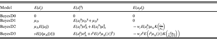
We consider the following submodels. The first submodel (BayesD0) contains only additive effects, so μd(|a j|)=0, σd2(|a j|, τj2)=0, and w j=0. Since w j=0, the putative additive effects a j have a t distribution with v degrees of freedom, mean 0 and variance ![]() if v>2. For v⩽2, the variance does not exist. If v is large, then the putative additive effects are approximately normally distributed. Note that BayesC of Verbyla et al. (Reference Verbyla, Bowman, Hayes and Goddard2010) appears as the special case where ε>0. Most of the Bayesian models mentioned in the introduction are also special cases or limiting cases of BayesD0.
if v>2. For v⩽2, the variance does not exist. If v is large, then the putative additive effects are approximately normally distributed. Note that BayesC of Verbyla et al. (Reference Verbyla, Bowman, Hayes and Goddard2010) appears as the special case where ε>0. Most of the Bayesian models mentioned in the introduction are also special cases or limiting cases of BayesD0.
In model BayesD1, additive effects and dominance effects are conditionally independent given τj2 with w j=0, μd(|a j|)=μD and σd2(|a j|,τj2)=s D2τj2, where s D>0. As a consequence, the distribution of the putative marker effect θj=(a j,d j) is elliptical.
In model BayesD2, absolute additive effects |a j| and dominance coefficients ![]() are independent. Thus, μd(|a j|)=|a j|μΔ and σd2(|a j|,τj2)=a j2σΔ2.
are independent. Thus, μd(|a j|)=|a j|μΔ and σd2(|a j|,τj2)=a j2σΔ2.
In model BayesD3, additive effects and dominance coefficients are dependent such that large additive effects are associated with large dominance coefficients. More precisely, we assume ![]() , where
, where ![]() with s Δ>0. Note that the function μΔ increases with μΔ(0)=0 and
with s Δ>0. Note that the function μΔ increases with μΔ(0)=0 and ![]() , so dominance coefficients of marker effects that are small in magnitude are centred at zero and dominance coefficients of marker effects that are large in magnitude are centred at one. Thus,
, so dominance coefficients of marker effects that are small in magnitude are centred at zero and dominance coefficients of marker effects that are large in magnitude are centred at one. Thus, ![]() , and σd2(|a j|,τj2)=a j2σΔ2.
, and σd2(|a j|,τj2)=a j2σΔ2.
The joint posterior distribution and the Markov chain
In this section, we present the joint posterior distribution for construction of the Markov chain. Since the Markov chain cannot be used for ε=0, we assume ε>0 in this section. In applications, the parameter ε would usually be chosen as small as possible in order to approximate a BayesB-type model. Alternatively, it could be chosen such that the accuracies of predicted BV and GV are maximized.
Let ξ=(β, u, σ2). We have p(ξ)∝p(u)p(σ2) because the assumption that β is a fixed effect is equivalent to the assumption that it has the flat prior p(β) ∝1. The joint posterior distribution is

where the likelihood function is
with ![]() . An explicit representation of the conditional prior distribution
. An explicit representation of the conditional prior distribution ![]() of the marker effects is needed in order to derive a Markov chain that uses this parameterization. We have
of the marker effects is needed in order to derive a Markov chain that uses this parameterization. We have
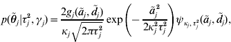
where κj=(1−γj)ε+γj,

and

Here, we used the abbreviation

The Markov chain for the prediction of the model parameters is generated by Gibbs sampling with a Metropolis–Hastings step. The algorithm is described in Appendix A. Starting with initial values, the parameters are sampled from their full conditional posterior distributions. The lengthy but straightforward proofs of the full conditional posterior distributions are given in the electronic appendix.
Moments of the random effects
Moments of the random effects given in this section are needed for the calculation of hyper-parameters. They are also needed for the calculation of the RKHS-kernel which is defined in the next section. For the second moment of a j to exist, we assume v>2. Since the putative marker effect θj and γj are independent, we have ![]() and
and ![]() for k∊{1, 2}. Moreover, we have
for k∊{1, 2}. Moreover, we have ![]() and
and ![]() , where E(κjk)=(1−p LD)εk+p LD. These formulae depend on moments of the putative marker effects. They can be calculated as
, where E(κjk)=(1−p LD)εk+p LD. These formulae depend on moments of the putative marker effects. They can be calculated as


where (Psarakis & Panaretos, Reference Psarakis and Panaretos1990):

φ is the cumulative distribution function of a standard normal distribution, and Γ is the Gamma function. The formulae can be further simplified for the considered submodels. Simplified formulae are given in Table 2, where t~t v has a t-distribution with v degrees of freedom.
Table 2. Model-specific expectations
Prediction of genotypic values
Take Ω={0, 1, 2}M to be the set of all possible multilocus genotypes at the M markers. For x∊Ω, x j is the number of 1-alleles at a particular marker j. According to the regression model described above, an individual with genotype x is assumed to have GV
provided that Z A is the gene content matrix with entries 0, 1, 2 and Z D is the indicator matrix for heterozygosity. That is, the GV is the sum of all additive effects and dominance effects that are carried by the individual. According to Falconer & Mackay (Reference Falconer and Mackay1996), the GV can be partitioned into a BV, a dominance deviation, and a contribution to the overall mean that is equal for all individuals. The BV is
and dominance deviation is
These are the formulae of Falconer & Mackay (Reference Falconer and Mackay1996, Table 7.3), except that summation is over the markers rather than over the QTLs.
Different methods are considered for the prediction of BV, dominance deviations and GV: the Bayesian methods explained above and an RKHS method. For the Bayesian methods, additive and dominance effects of the markers are predicted as posterior means from the MCMC algorithm. The predicted values are then inserted into the above equations to get the estimated genomic genotypic value EGV(x), the estimated genomic breeding value EBV(x) and the estimated genomic dominance deviation EDV(x).
In our paper, an RKHS method is used only for the prediction of GV. The kernel is derived from the assumptions of the regression model. Recall that the known genotypes are fixed explanatory variables. Randomness of GV arises from the randomness of allelic effects, so the function g GV(⋅) is random. Since RKHS regression assumes that GV are normally distributed with mean zero (Gianola & van Kaam, Reference Gianola and de los Campos2008), but ![]() , we cannot estimate g GV(⋅) directly. Instead, we estimate g(x)=g GV(x)−E(g GV(x)) with RKHS regression from the observations that are diminished by the expected GV. Then, an estimate of the GV is obtained as
, we cannot estimate g GV(⋅) directly. Instead, we estimate g(x)=g GV(x)−E(g GV(x)) with RKHS regression from the observations that are diminished by the expected GV. Then, an estimate of the GV is obtained as ![]() . For convenience, g(x) is also said to be a GV. The model assumptions imply that the covariance between GV of individuals with genotypes x and
. For convenience, g(x) is also said to be a GV. The model assumptions imply that the covariance between GV of individuals with genotypes x and ![]() is
is
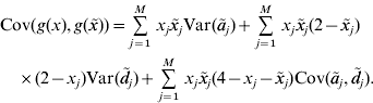
This equation defines the covariance matrix K for the GV of the phenotyped and genotyped individuals in the estimation set. Formulae for the calculation of the variances and covariances that appear on the right–hand side of the equation are given in the previous section. Then, the covariance matrix K can be calculated and used as a genomic relationship matrix for BLUP-prediction of GV. The resulting estimates are RKHS estimates (de los Campos et al., Reference de los Campos, Gianola and Rosa2009). Take ![]() to be the vector of predicted GV for individuals in the estimation set. It is used for the prediction of GV of non-phenotyped individuals as follows. For an individual with genotype x 0, the vector K 0 of covariances between the GV of this individual and the GV of all individuals in the estimation set can be calculated from equation (4). The estimated GV of the new individual is
to be the vector of predicted GV for individuals in the estimation set. It is used for the prediction of GV of non-phenotyped individuals as follows. For an individual with genotype x 0, the vector K 0 of covariances between the GV of this individual and the GV of all individuals in the estimation set can be calculated from equation (4). The estimated GV of the new individual is ![]() . Since x 0 was arbitrary, this equation defines an estimate
. Since x 0 was arbitrary, this equation defines an estimate ![]() of g. Note that the function
of g. Note that the function ![]() is symmetric and finitely positive-semidefinite because it is defined via a covariance function. The name RKHS regression results from the fact that a Hilbert space
is symmetric and finitely positive-semidefinite because it is defined via a covariance function. The name RKHS regression results from the fact that a Hilbert space ![]() exists for which the covariance function
exists for which the covariance function ![]() is a reproducing kernel. The Hilbert space is defined in Appendix C. The estimated function
is a reproducing kernel. The Hilbert space is defined in Appendix C. The estimated function ![]() belongs to this Hilbert space and is optimal in a well–defined sense among all functions that belong to this Hilbert space (Gianola & van Kaam, Reference Gianola and van Kaam2008).
belongs to this Hilbert space and is optimal in a well–defined sense among all functions that belong to this Hilbert space (Gianola & van Kaam, Reference Gianola and van Kaam2008).
This RKHS estimate is also the BLUP. Since all RKHS estimates are linear, it is the best estimate that can be obtained with RKHS regression, provided that the model assumptions are satisfied by the data and that the first two moments of the random effects are assumed known. In the applications, we calculated the kernel from the assumptions of BayesD2, so the RKHS estimate is nothing but the BLUP of BayesD2 (as opposed to the best predictor).
Calculation of hyper-parameters
For the calculation of the constant hyper-parameters, we assume whenever possible that additive variance, dominance variance and inbreeding depression of a random mating population are completely explained by the markers. This is not optimal because in fact, markers from low–density panels are not able to explain the total dominance variance. Thus, higher accuracies could be achieved when the parameters are chosen by a grid search or by cross validation. But we think that this is the natural way to choose the parameters. If the contribution of LD to the additive variance and the dominance variance are neglected, then expected additive variance V AM, dominance variance V DM and inbreeding depression ![]() M explained by markers are
M explained by markers are

where h j=2p jq j is the heterozygosity of marker j in the case of Hardy Weinberg equilibrium. Note that these formulae assume that the matrix Z A in the model specification denotes the gene content matrix and Z D is the indicator matrix for heterozygosity. The expectations can be calculated, which gives

where ![]() is the average heterozygosity,
is the average heterozygosity, ![]() is the average squared heterozygosity,
is the average squared heterozygosity, ![]() and
and ![]() .
.
For the model without dominance effects (BayesD0), the parameter s 2 is obtained from the condition V AM=V A, which gives

For the calculation of the fixed hyper-parameters for models that include dominance effects it is assumed that V A,V D and ![]() are known or have been estimated. Three parameters are chosen such that the conditions V AM=V A, V DM=V D and
are known or have been estimated. Three parameters are chosen such that the conditions V AM=V A, V DM=V D and ![]() M=
M=![]() hold. These are s 2, μD and s D2 for BayesD1, s 2, μΔ, σΔ2 for BayesD2, and s 2, s Δ, σΔ2 for BayesD3. The formulae for the calculation of these parameters are lengthy and are given in Appendix B.
hold. These are s 2, μD and s D2 for BayesD1, s 2, μΔ, σΔ2 for BayesD2, and s 2, s Δ, σΔ2 for BayesD3. The formulae for the calculation of these parameters are lengthy and are given in Appendix B.
Application
Simulation
A Fisher–Wright diploid population with population size N=1000 was simulated by sampling individuals for breeding with replacement for 5000 generations. Thereafter, the effective population size decreased for 400 generations from 1000 to 100 with a fast decrease in the most recent generations according to ![]() . This formula was chosen in order to reproduce the LD-pattern that is observed in cattle (compare with the estimated historic N e of cattle breeds, given in Villa-Angulo et al., Reference Villa-Angulo, Matukumalli, Gill, Choi, Van Tassell and Grefenstette2009). The total population size remained constant. This was achieved by reducing the number n mt of males and increasing the number n ft of females such that
. This formula was chosen in order to reproduce the LD-pattern that is observed in cattle (compare with the estimated historic N e of cattle breeds, given in Villa-Angulo et al., Reference Villa-Angulo, Matukumalli, Gill, Choi, Van Tassell and Grefenstette2009). The total population size remained constant. This was achieved by reducing the number n mt of males and increasing the number n ft of females such that ![]() .
.
The genome consisted of one chromosome of 1 Morgan with a mutation rate of 5×10⁻⁸. We simulated ten populations. For each population, ten traits with the same characteristics were simulated, so in total there were 100 replicates. In generation 0, 50 SNP for each trait were randomly selected among the about 84 000 segregating SNP to become a QTL. This corresponds to 1500 QTLs in a 30 Morgan genome. Additive and dominance effect of each QTL was sampled according to Scenario 3 fitted to PL in Wellmann & Bennewitz (Reference Wellmann and Bennewitz2011) . Thus, the QTL effects were sampled from the same distribution for all traits. Alleles with large effect tend to be partially recessive or dominant with heterozygous effect above the average effect of the two homozygotes. But alleles of small effect show highly variable dominance coefficients. The sign of the additive effect a j was chosen dependent on the allele frequency such that the contribution of the QTL to the additive variance is small, i.e. sign(a j)=−sign((q j−p j)d j). After additive and dominance effects had been sampled, they were rescaled by the same factor to obtain a heritability of h 2=V A=0·15 for each trait. Realized dominance variance and inbreeding depression varied considerably between traits because only one chromosome was simulated. Average dominance variance and inbreeding depression were ![]() and
and ![]() .
.
Starting with generation 1, the population was maintained without selection for five generations with N e,t=100 but N t=1000. The markers were identified in generation 1 based on the minor allele frequency (MAF) and on the distance to neighbouring markers. We considered three marker sets with 1500, 3000 and 6000 markers. This corresponds to 45 000, 90 000 and 180 000 markers in a 30 Morgan genome. Markers with high MAF were favoured. Average r 2-values between adjacent markers were similar for all marker sets. They ranged from 0·36 to 0·40. The marker effects were predicted once in generation 1 from 1000 individuals. Expected dominance variance V D=0·072 and inbreeding depression ![]() =0·59 were used as parameters to predict marker effects. Thus, the same hyper-parameters were used for all traits. Predicted marker effects were used to calculate estimated BV, dominance values and GV in generations 1–5. According to the scaling argument introduced by Meuwissen (Reference Meuwissen2009), the results can be extended to a population with a 30 Morgan genome and 30 000 individuals in the estimation set.
=0·59 were used as parameters to predict marker effects. Thus, the same hyper-parameters were used for all traits. Predicted marker effects were used to calculate estimated BV, dominance values and GV in generations 1–5. According to the scaling argument introduced by Meuwissen (Reference Meuwissen2009), the results can be extended to a population with a 30 Morgan genome and 30 000 individuals in the estimation set.
Analysis of the simulated data sets
We compared the accuracies that are obtained by the BayesD methods with G-BLUP, BayesA, BayesC and RKHS regression. Recall that BayesC does not contain dominance effects, BayesD1 assumes conditionally independent additive effect and dominance effects, BayesD2 assumes independent absolute additive effects and dominance coefficients, and BayesD3 assumes dependent absolute additive effects and dominance coefficients such that large additive effects are associated with large dominance coefficients.
G-BLUP and BayesA assume that all markers have a non-negligible effect, so p LD=1. For all other methods, we have chosen the scaling factor ε=0·01 and p LD depending on the marker panel. For marker panel k=1,2,3 with M=750×2k markers, we used p LD=0·8×0·35k. That is, we expected a priori that on average p LDM/50=12×0·7k markers are needed to capture the effect of one QTL for marker panel k. The formula for the calculation of p LD was chosen such that the expected number of required markers approaches the number of QTL when the size of the marker panel approaches the total number of SNP in the genome. For BayesD2 and BayesD3, we used w j=q j−p j. This parameter determines the probability that additive effect and dominance effect have the same sign for marker j. The degrees of freedom also had to be specified for each method. We used v=100 for G-BLUP, v=2·1 for BayesA, and v=2·5 for all other methods. The prior for the error variance was p(σ2)∝1/σ2. For simplicity, Xβ=1μ and Zu=0 were assumed. For BayesD1, the MCMC chains were run for 50 000 cycles and for all other methods, they were run for 10 000 cycles. The first 50% of the cycles were discarded. We used ten cycles in the Metropolis–Hastings step to sample the additive effects. Marker effects were estimated by the posterior means. The RKHS-regression estimate of the GV was calculated as described in Section (v). The reproducing kernel is defined by equation (4) and the underlying regression model is the same as for BayesD2, so the RKHS estimate has the property that it is the BLUP of BayesD2.
Results
Table 3 shows the accuracies of predicted BV, dominance deviations (DV) and GV for generation 2 and 5, where 3000 markers per chromosome are used. It also shows the regressions b BV, b DV and b GV of true BV, dominance deviations and GV on estimated values. Among all BayesD methods, BayesD3 yielded the highest accuracies and the regressions of true on predicted values are close to one. BayesD2 performed very similarly and was only slightly worse. In generation 2, BayesC yielded a 7% higher accuracy of predicted BV than G-BLUP and BayesD3 resulted in 10% higher accuracy. The accuracy of G-BLUP decreased by 10% from generation 2 to generation 5, whereas the accuracy of BayesD3 decreased only by 5%. As a consequence, BayesC had a 11% higher accuracy in generation 5, and BayesD3 had a 15% higher accuracy than G-BLUP. The methods differ very much in their ability to predict GV. The accuracy of GV in generation 2 was 15% less than the accuracy of BV if G-BLUP was used for the prediction, but it was only 3% less if BayesD3 was used. The accuracy of GV of BayesD3 exceeded that of G-BLUP by 26% in generation 2 and by 33% in generation 5. The accuracy of GV obtained from RKHS regression, exceeded that of G-BLUP by 4% in generation 2 and by 5% in generation 5. The choice of p LD and v did not affect the RKHS estimate (not shown). The results are visualized in Fig. 2. The figure shows the accuracies of predicted BV, dominance deviations and GV in generations 1–5 for the set with 3000 markers. It can be seen that the accuracy of the dominance deviation is below the accuracy of the BV. Interestingly, the accuracy of the dominance deviation decreases only very little from generation 1 to generation 5. This suggests that markers that capture the dominance effect of a QTL must be in high LD and therefore in close proximity of the QTL.

Fig. 2. Accuracy of predicted BV (a), dominance deviations (b) and GV (c) for generations 1–5 and 3000 markers per chromosome.
Table 3. Accuracies of predicted BV, dominance deviations (DV) and GV in generations 2 and 5, regressions bBV, bDV and bGV and of true on predicted values, and computation times per cycle relative to BayesA

Table 3 also shows that the BayesD methods required about twice as much computation time per cycle as the methods without dominance effects. This was expected because twice as many effects need to be predicted. The Metropolis–Hastings step that was needed to sample the additive effects in methods BayesD2 and BayesD3 increased the computation time only slightly. Figure 3 shows the mean accuracy of predicted GV in generations 1–5 when the sampler was stopped after 10, 100, 1000 or 10 000 cycles, and the first 50% of the cycles were discarded. GV were predicted from 3000 markers per chromosome. It can be seen that BayesA, BayesC, BayesD2 and BayesD3 approximately reached convergence after 1000 iterations, whereas BayesD1 may not have reached convergence, even after 10 000 iterations. The same applies for BV and dominance deviations.

Fig. 3. Mean accuracy of predicted GV in generations 1–5 calculated from 10x iterations of the sampler for 3000 markers per chromosome.
Figure 4 shows the mean accuracy of predicted BV, dominance deviations and GV in generations 1–5 for the different marker panels. Markers from high–density panels had a smaller MAF on average than markers from low–density panels, so they were less informative. This explains why the accuracies of G-BLUP, BayesA and BayesC increase only slightly for high–density panels. It can be seen that for an accurate prediction of dominance deviations and GV, high–density marker panels are needed. The likely reason for the increased accuracy of dominance deviations for high–density marker panels is, that the QTLs are on average in higher LD with a marker. For each QTL, we calculated the maximum r 2-value between the QTL and a marker. The average maximum r 2-values were 0·49, 0·64, and 0·80 for the different marker panels.

Fig. 4. Accuracy of predicted BV (a), dominance deviations (b), and GV (c) for marker panels with 1500, 3000 and 6000 markers per chromosome. The average maximum r 2 values of a QTL with a marker are shown on the x-axis for the different panels.
Discussion
New Bayesian models for the prediction of genomic BV, dominance deviations and GV have been introduced. The BayesD models outperformed BayesA and BayesC for the simulated data. BayesD3 and BayesD2, which both assume dependent additive and dominance effects, performed best. We showed that these methods not only enable an accurate prediction of BV, dominance deviations and GV, but they also lead to a smaller decrease of the accuracy of genomic BV in subsequent generations. Accuracies of genomic BV of BayesD methods were larger than the accuracies of methods that do not account for dominance. However, for an accurate prediction of dominance deviations and GV, high–density marker panels are needed. Computation time per predicted random effect was similar to BayesA. Interestingly, BayesD1 produced rather high accuracies even though the assumptions of this model were violated in the simulated data. For example, it did not take into account that dominance effects decreased rather than increased the additive variance of the population. However, it yielded smaller accuracies than the other BayesD methods and it showed a slower convergence of the Markov chain.
G-BLUP showed the strongest decrease of the accuracies in subsequent generations. This was expected because G-BLUP assumes normally distributed additive marker effects. This distribution is not heavy tailed. Therefore, more markers would be needed to capture the effect of one large QTL. These additional markers partly have a greater distance to the QTL, so recombinations can cause a greater drop in accuracy. BayesD3 showed the smallest decrease. Moreover, for the BayesD methods, the accuracy of the dominance deviations decreased only very little in subsequent generations. This suggests that a marker must be in strong LD with a QTL in order to capture the dominance effect of the QTL because otherwise, recombinations are likely to cause a faster decrease of the accuracies. As additive and dominance effects are dependent, and since both of them affect the BV of an individual, this could explain why the inclusion of dominance effects also slows the decrease in accuracy of genomic BV in subsequent generations, as shown in Fig. 2).
Since the BayesD2 estimate and the RKHS estimate (which is the BLUP of BayesD2) were derived from the same statistical model, it was expected that both methods provide similar accuracies. However, the increase in accuracies of GV over G-BLUP was much smaller for RKHS regression than for the Bayesian models. The reason is probably that RKHS regression could provide the best predictor if the GV are normally distributed, but this assumption was violated even though a relatively large number of QTLs was simulated. For RKHS regression, the increase in accuracy over G-BLUP was larger than the increases reported by other authors. Ober et al. (Reference Ober, Erbe, Long, Porcu, Schlather and Simianer2011) found that the accuracy in the validation set obtained with universal kriging was 0·013 larger than the accuracy of a genomic BLUP method. These authors chose the kernel from the family of Matérn covariance functions and additive variance and dominance variance were equal in the simulation. In our study, RKHS regression yielded a 0·027 higher accuracy than G-BLUP, although the dominance variance was only about half as large as the additive variance in our simulation. This suggests that a model-based definition of the kernel can increase the accuracies of RKHS regression estimates. A kernel that accounts for non-additive effects and uses SNP information was also proposed by Gianola & de los Campos (Reference Gianola and de los Campos2008) in analogy to the model of Henderson (Reference Henderson1985) which relies on the assumptions of Cockerham (Reference Cockerham1954) and Kempthorne (Reference Kempthorne1954) . In contrast to our model that assumes that the known genotypes are fixed and randomness of GV is due to randomness of the allelic effects, Cockerham and Kempthorne assumed implicitly that randomness of GV arises from randomness of the genotypes, and the function g that maps genotypes to GV is unknown and fixed. The joint distribution of the genotypes induces a covariance between GV that depends on the genetic architecture of the trait, i.e. on the unknown function g. Although it is often stated in the literature that g can be arbitrary, from these arguments it follows that RKHS regression makes strong assumptions about the genetic architecture of the trait because GV are inferred from the covariance structure of the GV, and the covariance structure depends on the genetic architecture. Gianola & de los Campos (Reference Gianola and de los Campos2008) stated that the choice of the kernel is indeed absolutely critical for attaining good predictions in RKHS regression.
If the number of markers is large and the prior probability p LD of a marker for being needed to capture a QTL effect is small, then the cumulative effect of all SNP drawn from the distribution with small variance can explain a considerable part of the variance even if ∊=0·01. But it is desirable that the model assumes only a small polygenic component if the marker density is large, so ∊ should be small in this case. However, a small ∊≪0·01 considerably slows convergence of the Markov chain, so one has to compromise. Alternatively, a BayesB-type algorithm that allows for ∊=0 may be used for this model.
The conditional variances τ j 2 were introduced only in order to obtain a hierarchical model that facilitates estimation of the marker effects with an MCMC algorithm. As noted by Gianola et al. (Reference Gianola, de los Campos, Hill, Manfredi and Fernando2009) for BayesA, these parameters cannot be estimated precisely from the data because the model does not allow Bayesian learning on these parameters. However, since they have no biological interpretation, estimates of these parameters are not needed.
There are several possibilities to further generalize our model. For example, the parameter s 2 could be different for each marker. That is, each marker could have its own variance. This could make sense in order to account for prior knowledge about a QTL that is in LD with the marker, or in order to account for the joint distribution of additive effects, dominance effects and allele frequencies. In the latter case, sj
2 would depend on the allele frequency of marker j. We assumed a folded t-distribution for the absolute values of the putative additive effects. As a consequence, we had to choose v>2 because otherwise the additive effects would have infinite variance. Since the degree of freedom v controls the thickness of the tails of a t-distribution, the choice of v could have a large effect on the accuracies. In this paper, this parameter was chosen by a grid search using cross validation. Alternatively, v could be treated as random and sampled with a Metropolis–Hastings step. Priors are proposed that assign a small probability to large values of v, but exclude v<2 (e.g. ![]() , see Rosa et al., Reference Rosa, Gianola and Padovani2004). The t-distribution could be modified to become a generalized hyperbolic distribution in order to force the variance of the additive effects to exist even for v<2.
, see Rosa et al., Reference Rosa, Gianola and Padovani2004). The t-distribution could be modified to become a generalized hyperbolic distribution in order to force the variance of the additive effects to exist even for v<2.
Different models may be appropriate for application depending on the objective of a study. If the aim of a study is the exploration of the genetic architecture of a quantitative trait then allelic effects may be predicted with different models and the assumptions of the model with the best predictive ability are likely to give a good description of the genetic architecture. However, it is unknown as to how epistasis would affect the predictive ability of the models, so inclusion of epistasis would be the logical next step. Alternatively, the genetic architecture could be explored by evaluation of the posterior distribution. In this case, BayesD1 may be the method of choice because it makes weak prior assumptions. Xu (Reference Xu2003) demonstrated that improper priors with heavy tails for additive and dominance effects produce clearer signals of QTL than the normal distribution. Therefore, small values of v and p LD could be preferable for QTL detection because this results in a more heavy–tailed distribution. If the aim of a study is the prediction of genomic BV or GV, then the model with best predictive ability should be chosen, provided that the computation time is acceptable. This is likely to be BayesD2 or BayesD3 because these models give the best fit to the genetic architectures that are suggested in the literature. Our simulation study confirms the superiority of BayesD2 and BayesD3. Similar joint distributions of additive effects and dominance effects were assumed for the simulation protocol and for BayesD3. If, contrary to our assumptions, the true joint distribution is very different for a trait (e.g. a trait with many overdominant alleles), then of course BayesD2 and BayesD3 would be not superior.
New methods have been introduced that enable computationally feasible, simultaneous and accurate prediction of BV, dominance deviations and GV for high–density marker sets. The number of females genotyped with a low–density marker set in dairy cattle breeds is increasing rapidly. High density marker genotypes or even whole genome sequences of sires and grandsires are becoming available for imputation. That is, high–density marker sets can be used for the prediction of BV and GV even though most individuals are only genotyped with a low–density marker set (Meuwissen & Goddard, Reference Meuwissen and Goddard2010a, Reference Meuwissen and Goddard2010b). Thus, the data needed to estimate dominance effects are becoming available. The conclusions drawn in this study are based on simulation experiments. The simulation protocol was designed to realistically model the dependencies between additive and dominance effects of QTLs for quantitative traits following the suggestions of Wellmann & Bennewitz (Reference Wellmann and Bennewitz2011) . Once real genomic data from traits with precise information on the genetic architecture including dominance effects become available, it should be used to validate the proposed models in the spirit of Hayes et al. (Reference Hayes, Pryce, Chamberlain, Bowman and Goddard2010) .
R. W. was supported by a grant from the Deutsche Forschungsgemeinschaft, DFG. The authors thank Christine Baes for language correction. The manuscript has benefited from the critical comments of the anonymous reviewers.
Appendix A: The Markov Chain
In this section, the Markov chain used for the prediction of the model parameters is described. In each cycle, the fixed effect β, the random effect u, the marker effects ![]() , the indicator variables γ1, …, γ
M
, the conditional variances
, the indicator variables γ1, …, γ
M
, the conditional variances ![]() , and the error variance σ2 are sampled (in this order). Details are described below.
, and the error variance σ2 are sampled (in this order). Details are described below.
Sampling of the fixed effect β
The full conditional posterior distribution of β is
where
In the special case where β=μ contains only the intercept, i.e. Xβ=1μ, the full conditional posterior simplifies to

Sampling of the random effect u
The full conditional posterior distribution of u is
where
Sampling of the marker effects 
We have
where

and ![]() is the density of a normal distribution with mean and variance
is the density of a normal distribution with mean and variance


where
Since ![]() if
if ![]() and
and ![]() if
if ![]() , a distribution with density proportional to
, a distribution with density proportional to ![]() is a mixture of two truncated normal distributions. Random numbers
is a mixture of two truncated normal distributions. Random numbers ![]() from h are needed as candidate values for the Metropolis–Hastings step that samples
from h are needed as candidate values for the Metropolis–Hastings step that samples ![]() . The probability p pos that a random variable with this distribution is positive equals
. The probability p pos that a random variable with this distribution is positive equals

where F is the cumulative distribution function with density f. Sampling of ![]() from h proceeds as follows:
from h proceeds as follows:
Sample I pos from
(1, p pos).If I pos=0 then sample U from
, else sample U from .Return
.
Here, ![]() denotes the uniform distribution on the interval [a, b]. The Metropolis–Hastings algorithm can be used to sample
denotes the uniform distribution on the interval [a, b]. The Metropolis–Hastings algorithm can be used to sample ![]() from the full conditional posterior as follows (Chib & Greenberg, Reference Chib and Greenberg1995):
from the full conditional posterior as follows (Chib & Greenberg, Reference Chib and Greenberg1995):
Sample
from hFor(i in 1:maxIt){
Sample
from hLet
With probability α let
}
Return
Note that the Metropolis–Hastings step is not needed if ![]() .
.
It remains to be shown how ![]() is sampled for models that include dominance effects. The full conditional posterior distribution of
is sampled for models that include dominance effects. The full conditional posterior distribution of ![]() is
is
where ![]() is the density of a normal distribution with mean and variance
is the density of a normal distribution with mean and variance

where
Since ![]() if
if ![]() and
and ![]() if
if ![]() , the full conditional posterior distribution of
, the full conditional posterior distribution of ![]() is a mixture of two truncated normal distributions. We have
is a mixture of two truncated normal distributions. We have

where ![]() is the cumulative distribution function with density
is the cumulative distribution function with density ![]() . Sampling of
. Sampling of ![]() proceeds as follows:
proceeds as follows:
Sample I pos from
.If I pos=0 then sample U from
, else sample U from .Return
.
Sampling of γ1, …, γM
The full conditional posterior distribution of γj is

where

Updating of γ1, …, γ M is only needed if p LD<1. After sampling of γ j , κ j needs to be updated.
Sampling of
For BayesD1, the full conditional posterior distribution of ![]() is
is

Otherwise, the full conditional posterior distribution of ![]() is
is

Sampling of the error variance σ2
The full conditional posterior distribution of σ2 is

where ![]() .
.
Appendix B: Calculation of hyper-parameters
For BayesD1 with conditionally independent additive effect and dominance effects the parameters s 2, μ D and sD need to be specified. We have

For BayesD2 with independent absolute additive effect and dominance coefficients the parameters s 2, μΔ and ![]() are obtained as follows. Since
are obtained as follows. Since

we can calculate ![]() . We have
. We have
where

Then ![]() can be calculated. Finally, s 2 is obtained from
can be calculated. Finally, s 2 is obtained from

For BayesD3 with dependent absolute additive effect and dominance coefficients, the parameters s 2, s Δ and ![]() are calculated as follows. At first, the parameter s Δ is determined such that the following equation holds:
are calculated as follows. At first, the parameter s Δ is determined such that the following equation holds:

where

This was done by a grid search, where the expectations were estimated from simulated random variables t~tv . Then σΔ2 can be calculated and s 2 is obtained from

Appendix C: Hilbert space for RKHS regression
This section defines the Hilbert space ![]() for which a symmetric and positive semidefinite kernel K is reproducing. Consider the linear space S that consists of all linear combinations of functions
for which a symmetric and positive semidefinite kernel K is reproducing. Consider the linear space S that consists of all linear combinations of functions ![]() with x∊Ω. Each function f∊S can be written as
with x∊Ω. Each function f∊S can be written as ![]() with N∊
with N∊![]() , pairwise different x 1, …, xN
∊Ω and a∊
, pairwise different x 1, …, xN
∊Ω and a∊![]() . For two functions
. For two functions ![]() , the inner product is defined as
, the inner product is defined as

S is a pre-Hilbert space with inner product 〈·, ·〉. The closure of S under the inner product 〈·, ·〉 is a Hilbert space ![]() . It is called the native space of the kernel K. Note that
. It is called the native space of the kernel K. Note that ![]() can be larger than S because it also includes all limiting functions of Cauchy sequences. The kernel K is a reproducing kernel of
can be larger than S because it also includes all limiting functions of Cauchy sequences. The kernel K is a reproducing kernel of ![]() . For proofs see the literature on Hilbert spaces, e.g. Shawe-Taylor & Cristianini (Reference Shawe-Taylor and Cristianini2004) .
. For proofs see the literature on Hilbert spaces, e.g. Shawe-Taylor & Cristianini (Reference Shawe-Taylor and Cristianini2004) .


