

Introduction
Modern macroevolutionary research resides at the nexus of paleontology and phylogenetic comparative biology. The fossil record provides a spectacular temporal window into the vicissitudes of life’s history, and paleontologists have long used its patterns to investigate large-scale trends in diversification dynamics and morphologic evolution over timescales inaccessible to experimental manipulation or field-based investigation (Simpson, Reference Simpson1944; Sepkoski, Reference Sepkoski1981; Hunt et al., Reference Hunt, Bell and Travis2008; Alroy, Reference Alroy2010). Similarly, biologists armed with molecular phylogenies of extant species and tree-based statistical techniques have increasingly become interested in addressing macroevolutionary questions traditionally studied by paleontologists (e.g., O’Meara et al., Reference O’Meara, Ané, Sanderson, Wainwright and Hansen2006; Bokma, Reference Bokma2008; Rabosky, Reference Rabosky2009; Rabosky and McCune, Reference Rabosky and McCune2009; Harmon et al., Reference Harmon, Losos, Davies, Gillespie and Gittleman2010; Pennell et al., Reference Pennell, Harmon and Uyeda2014). Although differences between paleontologic and biologic perspectives remain, attempts to bridge disciplinary gaps between fields have wide-reaching implications for assembling a more synthetic macroevolutionary theory (Jablonski, Reference Jablonski2008; Slater and Harmon, Reference Slater and Harmon2013; Hunt and Slater, Reference Hunt and Slater2016).
Instances of integration between fields, such as paleontology and molecular phylogenetics, often provide opportunities for reciprocal illumination. For example, fossils play a major role in dating divergences among extant species. Without external information to constrain absolute ages, branch length estimation is confounded by the fact that both rates of molecular sequence evolution and elapsed time contribute to observed distances among species. Thus, the construction of a time-calibrated molecular phylogeny requires information on fossil morphologies and their temporal distributions to provide a numerical timescale for testing alternative models of macroevolutionary dynamics (Donoghue and Benton, Reference Donoghue and Benton2007; dos Reis et al., 2016; Ksepka et al., Reference Ksepka, Parham, Allman, Benton, Carrano, Cranston, Donoghue, Head, Hermsen, Irmis and Joyce2015). Equally illuminating for paleontologists, many probabilistic methods originally developed by molecular phylogeneticists can be modified and applied to paleontologic data (Wagner, Reference Wagner2000a; Wagner and Marcot, Reference Wagner and Marcot2010; Lee and Palci, Reference Lee and Palci2015; but see Spencer and Wilberg, Reference Spencer and Wilberg2013). For example, Lewis (Reference Lewis2001) developed a k-state Markov model for calculating likelihoods of discrete, morphologic characters based on a generalization of the Jukes-Cantor model of molecular sequence evolution. Although simplistic, Lewis’s (Reference Lewis2001) ‘Mk’ model has recently been demonstrated in a Bayesian context to outperform other phylogenetic methods under a range of conditions present in real data sets, including missing character data, high rates of character evolution (and therefore homoplasy), and rate heterogeneity among characters (Wright and Hillis, Reference Wright and Hillis2014; O’Reilly et al., Reference O’Reilly, Puttick, Parry, Tanner, Tarver, Fleming, Pisani and Donoghue2016). The recent resurgence of ‘total-evidence’ (Pyron, Reference Pyron2011; Ronquist et al., Reference Ronquist, Klopfstein, Vilhelmsen, Schulmeister, Murray and Rasnitsyn2012) approaches in phylogenetics coincides with a renewed interest among biologists in phenotypic evolution and the utility of morphologic phylogenetics in an age of ‘post-molecular systematics’ (Lee and Palci, Reference Lee and Palci2015; Pyron, Reference Pyron2015). This revival of interest in morphologic phylogenetics is good news for paleontologists because nearly all phylogenies of fossil species are inferred using only morphologic character data. Indeed, there has been an increasing number of studies employing probabilistic approaches to estimate phylogenies with morphologic data, especially in paleontology (e.g., Wagner, Reference Wagner1998, Reference Wagner1999; Snively et al., Reference Snively, Russell and Powell2004; Pollitt et al., Reference Pollitt, Fortey and Wills2005; Clarke and Middleton, Reference Clarke and Middleton2008; Pyron, Reference Pyron2011; Ronquist et al., Reference Ronquist, Klopfstein, Vilhelmsen, Schulmeister, Murray and Rasnitsyn2012; Slater, Reference Slater2013, Reference Slater2015; Wright and Stigall, Reference Wright and Stigall2013; Lee et al., Reference Lee, Cau, Naish and Dyke2014; Close et al., Reference Close, Friedman, Lloyd and Benson2015; Bapst et al., Reference Bapst, Wright, Matzke and Lloyd2016; Gorscak and O’Connor, Reference Gorscak and O’Connor2016).
Particularly promising for systematic paleontology is the advent of tip-dating approaches for inferring phylogenies containing non-contemporaneous taxa (Pyron, Reference Pyron2011; Ronquist et al., Reference Ronquist, Klopfstein, Vilhelmsen, Schulmeister, Murray and Rasnitsyn2012; Gavryushkina et al., Reference Gavryshkina, Welch, Stadler and Drummond2014). Bayesian total-evidence tip-dating combines molecular sequences, morphologic character data, and temporal information on fossil distributions to simultaneously estimate the best tree topologies, branch lengths, and divergence times among extinct and extant lineages (Ronquist et al., Reference Ronquist, Klopfstein, Vilhelmsen, Schulmeister, Murray and Rasnitsyn2012; Lee and Palci, Reference Lee and Palci2015). Tip-dating approaches operate on the simple assumption that evolution can be modeled as a function of time, with either a strict or relaxed clock-like model of character change. Although most tip-dating studies combine fossil and living species (e.g., Pyron, Reference Pyron2011; Ronquist et al., Reference Ronquist, Klopfstein, Vilhelmsen, Schulmeister, Murray and Rasnitsyn2012; Slater, Reference Slater2013), tip-dating approaches equally apply to character matrices containing only morphologic data (Slater, Reference Slater2015) and/or with only fossil taxa (Lee et al., Reference Lee, Cau, Naish and Dyke2014; Bapst et al., Reference Bapst, Wright, Matzke and Lloyd2016; Gorscak and O’Connor, Reference Gorscak and O’Connor2016). Moreover, mathematical models originally developed for studying the spread of viruses in epidemiology have found applications in fossil tip-dating (Stadler et al., Reference Stadler, Kouyos, Wyl, von, Yerly, Böni, Bürgisser, Klimkait, Joos, Rieder, Xie, Günthard, Drummond and Bonhoeffer2012; Stadler and Yang, Reference Stadler and Yang2013; Gavryushkina et al., Reference Gavryshkina, Welch, Stadler and Drummond2014). The ‘fossilized birth–death’ process (Stadler, Reference Stadler2010; Heath et al., Reference Heath, Huelsenbeck and Stadler2014) has recently been applied within a Bayesian context as a more realistic tree prior distribution that accounts for macroevolutionary and sampling processes (Gavryushkina et al., Reference Gavryshkina, Welch, Stadler and Drummond2014).
This paper presents the first application of Bayesian tip-dating methods to a fossil-only data set of invertebrate animals. Here, I examine phylogenetic relationships among early to middle Paleozoic crinoids (Echinodermata). Crinoids are particularly amenable for the purposes herein because: (1) they have a well-sampled fossil record (Foote and Raup, Reference Foote and Raup1996); (2) their skeletal morphology is highly complex and character-rich (Ubaghs, Reference Ubaghs1978; Foote, Reference Foote1994; Ausich et al., Reference Ausich, Kammer, Rhenberg and Wright2015); and (3) testing phylogenetic hypotheses among crinoid higher taxa requires sampling non-contemporaneous taxa over long timescales (>107 years), making them an ideal system for implementing a tip-dating approach (Ronquist et al., Reference Ronquist, Klopfstein, Vilhelmsen, Schulmeister, Murray and Rasnitsyn2012). Because the approach taken herein is novel to the invertebrate fossil record, I provide a brief discussion on Bayesian tip-dating and the fossilized birth–death process tree prior to familiarize the reader with these emerging methods. Although this makes the paper necessarily technical in places, it is hoped those sections will provide a useful resource for other systematic paleontologists interested in probabilistic approaches to fossil phylogenetics.
Previous work on crinoid phylogeny
The Crinoidea form the sister group to all other extant echinoderm classes (Asteroidea, Echinoidea, Holothruoidea, and Ophiuroidea) and have an extensive geologic history spanning the Lower Ordovician (ca. 480 Ma) to the present day. Ever since Bather (Reference Bather1899) published his seminal work A Phylogenetic Classification of the Pelmatozoa, crinoid systematists have sought a robust evolutionary template for understanding the phylogenetic distribution of fossil and living species (Ausich and Kammer, Reference Ausich and Kammer2001). Other than a few isolated studies conducted at low taxonomic levels (e.g., Kammer, Reference Kammer2001; Gahn and Kammer, Reference Gahn and Kammer2002), most phylogenetic research using computational methods has focused on inferring relationships within two key time intervals: the Ordovician and the Recent (Ausich, Reference Ausich1998; Guensburg, Reference Guensburg2012; Hemery et al., Reference Hemery, Roux, Ameziane and Eleaume2013; Rouse et al., Reference Rouse, Jermiin, Wilson, Eeckhaut, Lanterbecq, Oji, Young, Browning, Cisternas, Helgen, Stuckey and Messing2013; Ausich et al., Reference Ausich, Kammer, Rhenberg and Wright2015; Summers et al., Reference Summers, Messing and Rouse2014; Cole, Reference Cole2017). These intervals are significant because they bookend the evolutionary history of crinoids into their early diversification during the Ordovician Period and their present-day diversity in marine ecosystems. However, these intervals are separated by ~480 million years, and phylogenetic research linking post-Ordovician stem taxa with the crown Crinoidea remains a largely unexplored area of research (Simms, Reference Simms1988; Simms and Sevastopulo, Reference Simms and Sevastopulo1993; Webster and Jell, Reference Webster and Jell1999).
Crinoids are traditionally divided into several higher taxa, including the Camerata, Disparida, Hybocrinida, Cladida, Flexibilia, and the Articulata (Moore and Teichert, Reference Moore and Teichert1978). Except for articulate crinoids, these groups first appear in Ordovician rocks. Despite more than a century of controversy, phylogenetic relationships among Ordovician taxa are reaching a consensus. For example, all recent analyses of Ordovician crinoids strongly support an early divergence between camerate and non-camerate crinoids (Guensburg, Reference Guensburg2012; Ausich et al., Reference Ausich, Kammer, Rhenberg and Wright2015; Cole, Reference Cole2017). Thus, the Camerata is the sister clade to all non-camerate crinoids. Similarly, both Guensburg (Reference Guensburg2012) and Ausich et al. (Reference Ausich, Kammer, Rhenberg and Wright2015) recovered a monophyletic Hybocrinida as the sister clade to a subset of cladid taxa. Ordovician analyses also recovered a monophyletic Disparida as sister to the clade of cyathocrine cladids and hybocrinids (Guensburg, Reference Guensburg2012; Ausich et al., Reference Ausich, Kammer, Rhenberg and Wright2015). However, relationships among taxa placed currently within the Cladida, and their relationships to other higher taxa, have been a long-standing problem in crinoid systematics (McIntosh, Reference McIntosh1986, Reference McIntosh2001; Sevastopulo and Lane, Reference Sevastopulo and Lane1988; Kammer and Ausich, Reference Kammer and Ausich1992, Reference Kammer and Ausich1996; Simms and Sevastopulo, Reference Simms and Sevastopulo1993).
In his review of echinoderm phylogeny and classification, Smith (Reference Smith1984) lamented the cladid portion of the crinoid tree was one of the “outstanding areas of ignorance in echinoderm phylogeny” (Smith, Reference Smith1984, p. 456). Indeed, the Cladida (sensu Moore and Laudon, Reference Moore and Laudon1943) have long been considered a paraphyletic group because some nominal cladids are hypothesized to be more closely related to flexible and/or articulate crinoids than other cladids (Springer, Reference Springer1920; Simms and Sevastopulo, Reference Simms and Sevastopulo1993; Brower, Reference Brower1995; Ausich, Reference Ausich1998; Wright, Reference Wright2015). Unfortunately, recent phylogenetic analyses not only confirm that Ordovician cladids are a paraphyletic assemblage (Guensburg, Reference Guensburg2012; Ausich et al., Reference Ausich, Kammer, Rhenberg and Wright2015), but also that the validity of the Cladida and their constituent higher taxa (i.e., Dendrocrinida and Cyathocrinida) cannot be fully remedied by simply adopting Simms and Sevastopulo’s (Reference Simms and Sevastopulo1993) recommendation to place the Flexibilia and Articulata within the Cladida. In addition, because the monophyletic status of a taxon requires a temporal reference frame (conventionally taken as the present day), it is unknown whether some recovered ‘clades’ in Ordovician analyses retain their monophyletic status when younger taxa are considered. For example, Ordovician cyathocrine cladids are typically recovered as a clade (Ausich, Reference Ausich1998; Ausich et al., Reference Ausich, Kammer, Rhenberg and Wright2015) but are sometimes nested within a more inclusive clade of cyathocrines and hybocrinids when hybocrinids are sampled in the same analysis. Testing whether the other cyathocrine cladids belong to this clade remains an open question and requires sampling younger species. Similarly, Ordovician cladids placed within the Dendrocrinida (sensu Moore and Laudon, Reference Moore and Laudon1943) are paraphyletic, but there may nevertheless be latent phylogenetic structure present among subsets of post-Ordovician dendrocrines that could inform taxonomic revisions.
The analyses conducted herein build on and further test recently proposed phylogenetic hypotheses that sample only Ordovician crinoids (Guensburg, Reference Guensburg2012; Ausich et al., Reference Ausich, Kammer, Rhenberg and Wright2015). This analysis includes a broad sample of early to middle Paleozoic (Ordovician–Devonian) non-camerate crinoids and primarily focuses on resolving relationships among the problematic Cladida.
Bayesian phylogenetics and the fossilized birth–death process
Bayesian phylogenetic methods combine a likelihood model of evolution with a set of prior probabilities to generate a posterior probability distribution of phylogenetic trees and their associated parameters. The Bayesian framework used herein is adapted from Gavryushkina et al. (Reference Gavryshkina, Heath, Ksepka, Stadler, Welch and Drummond2015). This model uses time-stamped morphologic character data to simultaneously estimate a posterior distribution of phylogenetic trees, divergence times, and other macroevolutionary and sampling parameters.
Let Ψ be a phylogeny (i.e., tree topology with branch lengths in units of time), δ be a vector of parameters describing morphologic evolution, and π be the tree prior (and its associated hyper parameters). Using Bayes theorem, the posterior probability distribution is
 $$f\left[ {\iPsi , \,\pi ,\, \delta \!\mid\! X,\, d} \right]{\equals} {{f[X\!\mid\!\iPsi , \delta ] \,f[d\!\mid\!\iPsi ]\,f\left[ {\iPsi \!\mid\!\pi } \right] \,f[\pi ]\,f[\delta ]} \over {f\left[ {X,\, d} \right]}} , $$
where X is a character by taxon matrix of morphologic character data and d is a vector of age ranges for each fossil taxon. The numerator on the right-hand side of the equation can be separated into the tree likelihood function,
 $f{\rm [}X{\rm \mid}\iPsi ,\,{\rm \delta }]$
, and the remaining terms, which comprises the prior. Equations for calculating
$f{\rm [}X{\rm \mid}\iPsi ,\,{\rm \delta }]$
, and the remaining terms, which comprises the prior. Equations for calculating
 $f{\rm [}X{\rm \mid}\iPsi ,\,{\rm \delta }]$
are well described in literature, and therefore a disquisition on tree likelihoods is not presented here. Interested readers are advised to see summaries in Swofford et al. (Reference Swofford, Olsen, Waddell and Hillis1996), Lewis (Reference Lewis2001), Felsenstein (Reference Felsenstein2004), and Yang (Reference Yang2014). The density
$f{\rm [}X{\rm \mid}\iPsi ,\,{\rm \delta }]$
are well described in literature, and therefore a disquisition on tree likelihoods is not presented here. Interested readers are advised to see summaries in Swofford et al. (Reference Swofford, Olsen, Waddell and Hillis1996), Lewis (Reference Lewis2001), Felsenstein (Reference Felsenstein2004), and Yang (Reference Yang2014). The density
 $f\left[ {\iPsi {\rm \mid\pi }} \right]$
describes the tree prior (see below) and
$f\left[ {\iPsi {\rm \mid\pi }} \right]$
describes the tree prior (see below) and
 $f\,{\rm [}d{\rm \mid}\iPsi ]$
is the density of obtaining fossil occurrence ranges given Ψ (this term is treated herein as a constant, see Gavryushkina et al., Reference Gavryshkina, Heath, Ksepka, Stadler, Welch and Drummond2015). The denominator f [X, d] is a normalizing constant and is equal to the marginal probability of the data. Given the necessary inputs, the posterior distribution of trees is estimated using a numerical technique called Markov chain Monte Carlo (MCMC) that eliminates the need to calculate f [X, d] when estimating the posterior distribution of trees.
$f\,{\rm [}d{\rm \mid}\iPsi ]$
is the density of obtaining fossil occurrence ranges given Ψ (this term is treated herein as a constant, see Gavryushkina et al., Reference Gavryshkina, Heath, Ksepka, Stadler, Welch and Drummond2015). The denominator f [X, d] is a normalizing constant and is equal to the marginal probability of the data. Given the necessary inputs, the posterior distribution of trees is estimated using a numerical technique called Markov chain Monte Carlo (MCMC) that eliminates the need to calculate f [X, d] when estimating the posterior distribution of trees.
A great strength of the Bayesian paradigm is that sources of uncertainty can be explicitly incorporated into the evolutionary model via the use of prior distributions on pertinent parameters (Heath and Moore, Reference Heath and Moore2014). For example, numerous factors can influence and potentially distort the accuracy of reconstructed evolutionary trees—arguably the most important parameter in phylogenetic inference. Even in cases where these other factors are not of primary interest, acknowledging and estimating ‘nuisance parameters’ is nevertheless important because it reduces the chance that any particular incorrect assumption will lead to the recovery of specious tree topologies (Huelsenbeck et al., Reference Huelsenbeck, Larget, Miller and Ronquist2002; Wagner and Marcot, Reference Wagner and Marcot2010; Gavryushkina et al., Reference Gavryshkina, Welch, Stadler and Drummond2014). Potential biasing factors may include variation in rates of morphologic evolution, taxonomic diversification rates, ancestor–descendant relationships, and (incompletely) sampling taxa over time rather than from a single time slice (Smith, Reference Smith1994; Wagner, Reference Wagner2000b, Reference Wagner2000c; Wagner and Marcot, Reference Wagner and Marcot2010; Bapst, Reference Bapst2012). Variability in evolutionary rates can be modeled with prior distributions to describe rate variation among characters. Similarly, rate variation among lineages can be modeled using uncorrelated ‘relaxed clock’ models where branch-specific rates are independently drawn from the same underlying parametric distribution (Lepage et al., Reference Lepage, Bryant, Philippe and Lartillot2007; Heath and Moore, Reference Heath and Moore2014).
Bayesian inference weights the likelihood of a tree by its prior probability. The fossilized birth–death (FBD) process (Stadler, Reference Stadler2010; Didier et al., Reference Didier, Royer-Carenzi and Laurin2012; Heath et al., Reference Heath, Huelsenbeck and Stadler2014) is an extension of the constant rate birth–death models commonly used in paleontology (e.g., Raup et al., Reference Raup, Gould, Schopf and Simberloff1973; Raup, Reference Raup1985) and considers fossil preservation in addition to diversification dynamics. In the following, I briefly describe the FBD process as a tree prior and argue it is well suited to accommodate these additional sources of concern.
Tree prior
The fossilized birth–death (FBD) process is a stochastic branching model for describing macroevolutionary dynamics, fossil preservation, and sampling (Stadler, Reference Stadler2010; Heath et al., Reference Heath, Huelsenbeck and Stadler2014). The FBD process begins at some time t o > 0 in the past and ends when t=0. As time moves forward (i.e., decreasing toward the ‘present’), each lineage may probabilistically undergo one of three process-based events, each according to a distinct constant rate Poisson process: branching (i.e., lineage splitting via speciation) with rate p, extinction with rate q, or fossil preservation and sampling with rate r (Stadler, Reference Stadler2010; Heath et al., Reference Heath, Huelsenbeck and Stadler2014). Lineages alive at the end of the process are sampled with probability ε corresponding to the sampling fraction of ‘extant’ taxa. It is important to note that the start and end times for the FBD process are arbitrary, and time can therefore be shifted to accommodate temporal frameworks more commonly used in paleontology. For example, paleontological systematists working on entirely extinct groups (e.g., trilobites) or sampling taxa from a restricted temporal interval (e.g., Paleozoic crinoids) can shift time such that t=0 corresponds to the age of the youngest species sampled. The FBD process represents a major advance over other birth–death models in paleontology (e.g., Raup, Reference Raup1985) because fossil preservation and sampling issues are modeled in addition to clade diversification. In the implementation of Gavryushkina et al. (Reference Gavryshkina, Welch, Stadler and Drummond2014), a lineage may be sampled more than once, thereby producing an internal node connected to only two (rather than three) branches. A two-degree internal node in a phylogenetic tree implies a hypothesized ancestor–descendent relationship, via direct or indirect ancestry (Fig. 1) (Foote, Reference Foote1996; Gavryushkina et al., Reference Gavryshkina, Welch, Stadler and Drummond2014, Reference Gavryshkina, Heath, Ksepka, Stadler, Welch and Drummond2015).

Figure 1 Illustration of the fossilized birth–death process. (1) A full realization of the FBD process from time t in the past to the end of the process. Diversification produces a tree with branching and extinction events and random sampling of nodes. Sampling events are indicated by dots. (2) A ‘reconstructed’ phylogenetic tree produced by pruning all of the unsampled lineages in 1.1. Thus, only the observed portion of samples participating in the macroevolutionary process is depicted. Note that some sampled nodes represent ancestors.
The set of stochastic branching, extinction, and sampling events for a single FBD process gives rise to a ‘complete’ phylogeny with generating parameters π=(p, q, r, ε, t
o
) (Fig. 1.1). The ‘sampled’ FBD phylogeny is obtained when all lineages with unsampled descendants produced by the process are pruned from the tree and therefore represents the reconstructed tree topology and divergence times implied by the sampled taxa (Fig. 1.2). Trees sampled from the FBD process are called sampled ancestor phylogenetic trees (even if no ancestors were sampled), and their nodes can be labeled to summarize their unique history of macroevolutionary and sampling events (Gavryushkina et al., Reference Gavryshkina, Welch, Stadler and Drummond2014). Equations for calculating the probability density of
 $f\left[ {\iPsi {\rm \mid\pi }} \right]$
given the FBD parameters p, q, r, and ε can be derived by modifying birth–death sampling models used to study virus transmissions in epidemiology (Stadler, Reference Stadler2010; Stadler et al., Reference Stadler, Kouyos, Wyl, von, Yerly, Böni, Bürgisser, Klimkait, Joos, Rieder, Xie, Günthard, Drummond and Bonhoeffer2012; Gavryushkina et al., Reference Gavryshkina, Welch, Stadler and Drummond2014; Zhang et al., Reference Zhang, Stadler, Klopfstein, Heath and Ronquist2016), and their details are discussed in the Appendix.
$f\left[ {\iPsi {\rm \mid\pi }} \right]$
given the FBD parameters p, q, r, and ε can be derived by modifying birth–death sampling models used to study virus transmissions in epidemiology (Stadler, Reference Stadler2010; Stadler et al., Reference Stadler, Kouyos, Wyl, von, Yerly, Böni, Bürgisser, Klimkait, Joos, Rieder, Xie, Günthard, Drummond and Bonhoeffer2012; Gavryushkina et al., Reference Gavryshkina, Welch, Stadler and Drummond2014; Zhang et al., Reference Zhang, Stadler, Klopfstein, Heath and Ronquist2016), and their details are discussed in the Appendix.
Taxon sampling, characters analyzed, and specimens examined
The character matrix analyzed herein was constructed as part of a larger project resolving phylogenetic relationships among Paleozoic crinoids. I updated, modified, and expanded the character list of Ausich et al. (Reference Ausich, Kammer, Rhenberg and Wright2015) to include an ensemble of new characters to better capture variation among post-Ordovician taxa, particularly among ‘cladids’ (Ausich et al., Reference Ausich, Kammer, Rhenberg and Wright2015; Wright and Ausich, Reference Wright and Ausich2015). Because the taxonomic diversity of fossil crinoids is formidably high for comprehensive analysis, taxon sampling was restricted to Ordovician through Devonian species and multiple exemplars were sampled at pertinent taxonomic scales appropriate to the present analysis (Brusatte, Reference Brusatte2010). The matrix was constructed in an attempt to maximize sampling across the broad spectrum of taxonomic, morphologic, and preservation gradients while keeping rigorous analysis tractable (Wagner, Reference Wagner2000c; Carlson and Fitzgerald, Reference Carlson and Fitzgerald2007; Heath et al., Reference Heath, Hedtke and Hillis2008).
The data set contains representative species from Ordovician, Silurian, and Devonian families of nominal ‘cladids’ (including cyathocrines and dendrocrines), disparids, hybocrinids, and flexibles (all taxa sensu Moore and Laudon, Reference Moore and Laudon1943). Species chosen as exemplars were typically the type species of a type genus that well characterizes the distribution of morphologic traits for each higher taxon, but sometimes geologically older species and/or more complete specimens were sampled instead (Table 1). Characters, plate homologies, and terminology are after Ubaghs (Reference Ubaghs1978) and Ausich et al. (Reference Ausich, Kammer, Rhenberg and Wright2015), with updates from Webster and Maples (Reference Webster and Maples2006) and Wright (Reference Wright2015). All but four traits were treated as unordered binary or multistate characters (Supplemental Data 1). These four characters were ordered based on known patterns of crinoid development, and arguments for ordering these traits are discussed by Wright (Reference Wright2015) and Webster and Maples (Reference Webster and Maples2006, Reference Webster and Maples2008). Unknown and inapplicable character states were coded as missing. This new compilation of more than 3,000 specimen-based observations is the largest and most comprehensive morphologic data matrix ever constructed sampling Ordovician and post-Ordovician fossil crinoids (Supplemental Data 2).
Table 1 Species sampled for phylogenetic analysis.
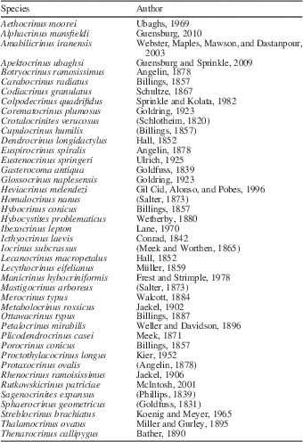
In the final matrix, a total of 87 discrete morphologic characters comprising more than 300 character states were sampled across 42 species of non-camerate crinoids (Supplemental Data 2). Camerates were not included in the analysis because they diverged from non-camerate crinoids by at least the earliest Ordovician (Guensburg and Sprinkle, Reference Guensburg and Sprinkle2003; Guensburg, Reference Guensburg2012; Ausich et al., Reference Ausich, Kammer, Rhenberg and Wright2015; Cole, Reference Cole2017). Although tip-dating analyses do not per se require use of an outgroup (Ronquist et al., Reference Ronquist, Klopfstein, Vilhelmsen, Schulmeister, Murray and Rasnitsyn2012), there are several reasons I used the Tremodocian species Apektocrinus ubaghsi Guensburg and Sprinkle, Reference Guensburg and Sprinkle2009 to assist rooting the tree. Apektocrinus was originally described as a tentative cladid that featured traits intermediate between protocrinoids and nominal cladids (Guensburg and Sprinkle, Reference Guensburg and Sprinkle2009). Protocrinoids were originally considered basal crinoids stemward of the divergence between camerates and non-camerates (Guensburg and Sprinkle, Reference Guensburg and Sprinkle2003). However, Guensburg (Reference Guensburg2012) subsequently placed protocrinoids within the Camerata, and later analyses by Ausich et al. (Reference Ausich, Kammer, Rhenberg and Wright2015) recovered protocrinoids to be closer to non-camerates than to camerates. Regardless of the labile phylogenetic position of protocrinids, both Guensburg (Reference Guensburg2012) and Ausich et al. (Reference Ausich, Kammer, Rhenberg and Wright2015) recovered tree topologies with Apektocrinus as the sister taxon to the clade comprised of non-camerate crinoids. Thus, the early stratigraphic position, mosaic distribution of plesiomorphic and apomorphic traits, and strong support from previous phylogenetic analyses all indicate Apektocrinus occupies a position near the base of the non-camerate tree (Guensburg and Sprinkle, Reference Guensburg and Sprinkle2009; Guensburg, Reference Guensburg2012; Ausich et al., Reference Ausich, Kammer, Rhenberg and Wright2015).
Matrix construction required extensive first-hand examination of well-preserved specimens housed in museum collections and of the published taxonomic literature. When possible, I coded characters from direct observations of type-series specimens for each species. Although emphasis was placed on observing characters from type specimens, non–type specimens were also examined to ensure the character distributions for each species were coded as completely as possible. Specimens were examined from collections within the United States National Museum of Natural History, the Field Museum of Natural History, the Lapworth Museum of Geology, and the Natural History Museum (London).
Phylogenetic analyses
Bayesian phylogenetic analyses were conducted using Markov chain Monte Carlo (MCMC) sampling in the MPI-version of MrBayes 3.2.5 (Ronquist et al., Reference Ronquist, Klopfstein, Vilhelmsen, Schulmeister, Murray and Rasnitsyn2012), which implements MCMC proposals for FBD trees (Zhang et al., Reference Zhang, Stadler, Klopfstein, Heath and Ronquist2016). To account for differences among alternative model configurations, multiple phylogenetic analyses were conducted and Bayes factors (BFs) were calculated to statistically compare models. Bayes factors are used in Bayesian model selection to determine which parameter configurations provide the best fit to the data and are equal to twice the difference in marginal log-likelihoods between models (Kass and Raftery, Reference Kass and Raftery1995). Following phylogenetic analyses, I then estimated the marginal log-likelihood of each model using the stepping-stone sampling method (Xie et al., Reference Xie, Lewis, Fan, Kuo and Chen2010) with 50 steps and powers of β corresponding to quantiles of a Beta(0.5, 1.0) distribution. Parsimony-based calculations were performed using PAUP* 4.0a147 (Swofford, Reference Swofford2002). All additional analyses were conducted using custom scripts written in the R statistical computing environment making use of functions from the packages APE (Paradis et al., Reference Paradis, Claude and Strimmer2004), and STRAP (Bell and Lloyd, Reference Bell and Lloyd2015). Details regarding choices of prior distributions, constraints, and MCMC convergence are discussed in the following.
Morphologic character evolution was modeled using the Mk model with equal transition frequencies among character states and a correction for ascertainment bias in character acquisition (Lewis, Reference Lewis2001). The distribution of rates among characters can assume either a uniform ‘equal rates’ model or explicitly account for rate heterogeneity using a skewed parametric distribution. A preliminary parsimony-based estimation of rate variation in the crinoid character matrix depicts a highly skewed distribution (Fig. 2), strongly suggesting it is unwise to assume a model of equal rates of change among characters. This is particularly striking given that parsimony-based rate distributions tend to underestimate morphologic changes and are therefore slightly biased toward equal rates (Harrison and Larsson, Reference Harrison and Larsson2015). To further test this hypothesis, I conducted separate analyses assuming equal, lognormal, and gamma distributed rates of character change. Following Harrison and Larsson’s (Reference Harrison and Larsson2015) recommendation, analyses with gamma or lognormal variation used eight instead of four discrete rate categories (commonly applied to molecular data).

Figure 2 Parsimony-based estimate of rate variation among characters. This distribution suggests that many characters evolve slowly, whereas a small number of characters evolve at much higher rates.
Fossil tip-dating requires a model characterizing the distribution of evolutionary rates throughout the tree. The case of a strict-morphological clock assumes rates are constant among lineages. However, the assumption of the strict-clock can be ‘relaxed’ by allowing rates to vary among branches throughout the tree (Lepage et al., Reference Lepage, Bryant, Philippe and Lartillot2007; Heath and Moore, Reference Heath and Moore2014). To test whether evolutionary rates vary among lineages, strict- and relaxed-clock analyses were conducted. The independent gamma rates (IGR) relaxed-clock model was applied to account for variation in rates among branches. The IGR model facilitates episodic ‘white noise’ variation in rates across the tree and is appropriate because large-scale morphologic evolution is a function of both waiting times and stochastic selective forces (Wagner, Reference Wagner2012; Heath and Moore, Reference Heath and Moore2014). A lognormal distribution was placed on the base rate of the clock using methods outlined by Ronquist et al. (Reference Ronquist, Klopfstein, Vilhelmsen, Schulmeister, Murray and Rasnitsyn2012).
A key assumption of tip-dating is that evolutionary change is a function of time. In other words, geologically younger species are expected to have undergone a greater amount of within-lineage evolution (i.e., anagenesis) than older species because more time has elapsed for changes to occur (Smith et al., Reference Smith, Lafay and Christen1992; Wagner, Reference Wagner2000a). To test whether this assumption holds (and therefore whether the tip-dating method is valid for these data), the parsimony-based root-to-tip path length of each species from a non-clock analysis was regressed against median age dates from the IGR analysis using both phylogenetically corrected and uncorrected methods (Lee et al., Reference Lee, Cau, Naish and Dyke2014).
The FBD process was used as a tree prior (i.e., ‘samplestrat=random’ in MrBayes 3.2.5). The implementation of the FBD in MrBayes reparameterizes the FBD process in terms of net diversification (=p–q), turnover (=q/p), and sampling probability (=r/(q+r). I placed an Exp(1) prior on net diversification, a Beta(1,1) uniform prior on turnover, and a Beta(2,2) prior on the sampling probability. To account for uncertainty in divergence time estimation, age ranges for fossil species were given broad uniform distributions typically corresponding to the stratigraphic range of their higher taxon and were taken from an updated version of Webster’s (Reference Webster2003) index of Paleozoic crinoids (Supplemental Data 2). Because the age of the most recent common ancestor of all species in the analysis is well constrained by fossil evidence to be near the base of the Ordovician, the tree age prior was fixed to correspond to the earliest Tremadocian.
Tip-dating is a computationally demanding phylogenetic method that requires a time-consuming exploration of parameter space. To assist the analysis, several topological constraints were applied to reduce MCMC exploration of very unlikely trees and to test more specific phylogenetic hypotheses (see Guillerme and Cooper, Reference Guillerme and Cooper2016). For example, the monophyly of disparids and flexibles are well supported by other studies (Brower, Reference Brower1995; Ausich, Reference Ausich1998; Guensburg, Reference Guensburg2012; Ausich et al., Reference Ausich, Kammer, Rhenberg and Wright2015) and preliminary analyses. Thus, their status as clades is not in question. However, the branching position of these clades within the larger crinoid tree remains an open question, and their phylogenetic placement is evaluated herein. A partial constraint was placed on Eustenocrinus, Iocrinus, Ibexocrinus, and Heviacrinus that allowed for either Merocrinus and/or Alphacrinus to be included within the disparid clade if the data support that hypothesis. This was done because whether Merocrinus is closer to cladids or disparids requires additional testing (cf. Ausich, Reference Ausich1998; Guensburg, Reference Guensburg2012). Alphacrinus is a stratigraphically old taxon with a combination of unique and disparid-like traits that may or may not be stemward to ingroup Disparida (Guensburg, Reference Guensburg2010). A hard constraint was placed on a flexible clade comprising Homalocrinus, Icthyocrinus, Lecanocrinus, Protaxocrinus, and Sagenocrinites.
Markov chain Monte Carlo analyses consisted of two independent runs of four chains sampling every 4,000 generations for 40 million generations per run with a burn-in percentage of 35%. Convergence was assessed using multiple criteria: average standard deviation of split frequencies among chains were below 0.01 (<0.05 for some IGR analyses) (Gelman and Rubin, Reference Gelman and Rubin1992), potential scale reduction factors of ~1.0 (Lakner et al., Reference Lakner, van der Mark, Huelsenbeck, Larget and Ronquist2008), effective sample sizes greater than 300 (with many >1,000), and visual inspection of log-likelihood plots among runs using Tracer v.1.6 (Drummond and Rambaut, Reference Drummond and Rambaut2007). Finally, the analysis with the best fit parameter settings was repeated three times to ensure estimates of optimal tree topologies were robust across runs. Together, these diagnostics indicate convergence among tree topologies and parameter estimates.
To summarize the posterior distribution of tree topologies, I generated a maximum clade credibility (MCC) tree using TreeAnnotator (Rambaut and Drummond, Reference Rambaut and Drummond2015). Although there is no single agreed-upon method for summarizing Bayesian posterior distributions of phylogenetic trees (Heled and Bouckaert, Reference Heled and Bouckaert2013), posterior probability can be viewed as an optimality criterion in phylogenetic inference (Rannala and Yang, Reference Rannala and Yang1996; Huelsenbeck et al., Reference Huelsenbeck, Larget, Miller and Ronquist2002; Wheeler and Pickett, Reference Wheeler and Pickett2007; Wheeler, Reference Wheeler2012; Rambaut, Reference Rambaut2014). The MCC tree is the tree in the posterior distribution with the maximum product of clade posterior probabilities and represents a Bayesian point estimate of phylogeny (Rambaut, Reference Rambaut2014).
I also ran a series of sensitivity analyses (n>5) to explore the effects of choosing different priors, including the prior placed: (1) on the variance of the gamma distribution in the IGR model, and (2) on the FBD turnover (= q/p) parameter. In all cases, statistically indistinguishable median estimates were obtained for node ages, branch lengths, and FDB parameters. In addition, I calculated the pairwise Robinson-Foulds (RF) distance (Robinson and Foulds, Reference Robinson and Foulds1981) within and among tree distributions from separate analyses and ordinated the resulting RF matrix using principal coordinate analysis. A visual inspection of RF distances in principal coordinate space reveals substantial overlap between distributions, with no obvious gradient or isolated ‘islands’ (analogous to Maddison, Reference Maddison1991) of trees. Thus, the analysis presented herein is considered robust across a range of possible prior configurations.
Results
The relationship between within-lineage morphologic evolution and IGR age estimates indicates early to middle Paleozoic crinoids conform well to the assumptions of tip-dating. Parsimony-based branch lengths from a non-clock analysis reveals geologically younger taxa have higher amounts of anagenesis compared to older taxa (p=0.017) (Fig. 3). This relationship holds even when accounting for phylogenetic non-independence among comparisons, as phylogenetic independent contrasts (Felsenstein, Reference Felsenstein1985) also reveal a strong statistical association between branch durations (in the best-fit IGR analysis) and morphologic divergence (measured in parsimony steps from an undated analysis) (p=0.005) (see Lee et al., Reference Lee, Cau, Naish and Dyke2014).

Figure 3 Testing statistical associations between the amount of morphologic evolution inferred from an undated analysis and divergence times estimated under a relaxed morphologic-clock model: (1) node age in millions of years and anagenesis (measured as the total root-to-tip distance in parsimony steps from an undated analysis); (2) phylogenetic independent contrasts between branch durations (from time-scaled analysis) and anagenesis (from an undated analysis). Both regressions are statistically significant.
Bayes factors provide evidence for heterotachy in crinoid evolution throughout this interval (Supplemental Data 3). The equal rates model of character evolution was strongly rejected in favor of models incorporating rate variation (BF=166.42 for lognormal, BF=162.04 for gamma), with the lognormal slightly outperforming a gamma distribution (BF=4.38). Similarly, the strict-morphological clock was strongly rejected in favor of the IGR relaxed-clock model accounting rate variation among lineages (BF=54.56).
The MCC tree from the best fit model is presented in Figure 4. Although posterior probabilities for some clades are low, they are comparable to other tip-dating studies using morphologic characters (Lee et al., Reference Lee, Cau, Naish and Dyke2014; Gavryushkina et al., Reference Gavryshkina, Heath, Ksepka, Stadler, Welch and Drummond2015; Gorscak and O’Connor, Reference Gorscak and O’Connor2016). Because Bayesian analyses account for uncertainty in the phylogenetic placement of taxa, it is important to stress that relationships depicted in Figure 4 are not the only ones supported in the posterior distribution. However, MCC tree topologies were broadly consistent across all analyses, indicating topological results are robust across different model configurations. Keeping uncertainty in mind, there are many salient features of the MCC tree that support previous phylogenetic hypotheses and throw light on several taxonomic questions.

Figure 4 Maximum Clade Credibility tree of early to middle Paleozoic crinoids. Posterior probabilities (>.50) are located next to nodes and expressed in percent; blue node bars represent the 95% highest posterior density age estimates; thick black bars represent genus-level stratigraphic ranges. Note the inclusion of stratigraphic ranges gives the appearance of sister taxon relationships where zero-length branches were sampled (e.g., Cupulocrinus). The Cladida (sensu Simms and Sevastopulo, Reference Simms and Sevastopulo1993) are sister to the Disparida. Crinoid taxa depicted represent the major clades discussed in the text: (from top to bottom) the disparid Eustenocrinus springeri Ulrich, Reference Ulrich1925, redrawn from Ubaghs (Reference Ubaghs1978); representative porocrinoid and hybocrinid (see text), Hybocrinus conicus Billings, Reference Billings1857, redrawn from Sprinkle and Moore (Reference Sprinkle and Moore1978); the flexible Protaxocrinus laevis (Billings, Reference Billings1857), redrawn from Springer (Reference Springer1911); representative eucladid Dictenocrinus, redrawn from Bather (Reference Bather1900).
The base of the MCC tree is characterized by a basal divergence between disparids (and disparid-like taxa) and all other non-camerate crinoids. Neither Merocrinus nor Alphacrinus were placed within the clade comprising Iocrinus, Ibexocrinus, Eustenocrinus, and Heviacrinus. However, Merocrinus is placed as the sister taxon to Metabolocrinus, which together form a sister clade to the above-mentioned disparid clade. It is interesting to note that Alphacrinus is placed as the sister taxon to the clade comprised of Merocrinus, Metabolocrinus, and disparids, which supports Guensburg’s (Reference Guensburg2010) original hypothesis of Alphacrinus being a basal disparid-like taxon and contrasts with Guensburg’s (Reference Guensburg2012) subsequent analysis recovering Alphacrinus as nested within the disparid clade.
Similar to other studies (Ausich, Reference Ausich1998; Guensburg, Reference Guensburg2012; Ausich et al., Reference Ausich, Kammer, Rhenberg and Wright2015), a clade comprised of cladids and hybocrinids was recovered. This clade is strongly supported with posterior probability 0.96. The hybocrinids Hybocrinus and Hybocystites are sister taxa and occupy a nested position within a clade of dicyclic ‘cyathocrine’ cladids (i.e., Carabocrinus and Porocrinus), suggesting these taxa are pseudomonocyclic (Sprinkle, Reference Sprinkle1982; Guensubrg, 2012; Ausich et al., Reference Ausich, Kammer, Rhenberg and Wright2015).
A clade comprised of Cupulocrinus and flexible crinoids was recovered as sister to a clade comprised of only cladids, with the inclusive clade supported with posterior probability 0.65. Although Cupulocrinus is a nominal cladid (sensu Moore and Laudon, Reference Moore and Laudon1943), it is placed closer to flexibles than other cladids in 96% of trees in the posterior distribution.
The large clade comprising the most recent common ancestor of Plicodendrocrinus and Corematocrinus and its descendants contains a scattering of taxa traditionally placed within the cladid orders Cyathocrinida and Dendrocrinida (sensu Moore and Laudon, Reference Moore and Laudon1943). Thus, the traditionally recognized ‘cyathocrine’ and ‘dendrocrine’ cladids represent evolutionary grades of body plan organization rather than clades. For example, a clade of cyathocrine-grade crinoids containing the most recent common of Thalamocrinus and Gasterocoma is supported with posterior probability 0.80, with subclades supported by posterior probabilities between 0.53 and 0.75. Similarly, a different clade containing the most recent common ancestor of Lecythocrinus and Petalocrinus also features ‘cyathocrine’ morphologies. These results support (perhaps unfortunately) long-held suspicions of taxonomic anarchy among cladids recognized by previous authors (McIntosh, Reference McIntosh1986, Reference McIntosh2001; Kammer and Ausich, Reference Kammer and Ausich1992, Reference Kammer and Ausich1996; Simms and Sevastopulo, Reference Simms and Sevastopulo1993; Webster and Maples, Reference Webster and Maples2006).
The clade of dendrocrine-grade crinoids containing the most recent common ancestor of Thenarocrinus and Corematocrinus, and its constituent subclades, are supported with posterior probabilities between 0.68 and 0.84. This clade contains a subclade comprising members of the Rutkowskicrinidae, Glossocrinidae, Corematocrinidae, and Amabilicrinidae. This clade is supported with posterior probability 0.84 and is equivalent to the superfamily Glossocrinacea originally recognized by Webster et al. (Reference Webster, Maples, Mawson and Dastanpour2003).
Discussion
It is generally appreciated that quantitative phylogenetic methods do not typically take full advantage of the complete spectrum of information supplied by the fossil record (Wagner and Marcot, Reference Wagner and Marcot2010). However, recently developed probabilistic macroevolutionary models and powerful computational tools have provided major advancements for estimating phylogenies containing fossil taxa and accommodating paleontologic idiosyncrasies, such as sampling taxa (incompletely) over time (Stadler, Reference Stadler2010; Ronquist et al., Reference Ronquist, Klopfstein, Vilhelmsen, Schulmeister, Murray and Rasnitsyn2012; Gavryushkina et al., Reference Gavryshkina, Welch, Stadler and Drummond2014; Lee and Palci, Reference Lee and Palci2015). This paper builds on these advances by implementing a Bayesian framework to estimate time-scaled phylogenetic hypotheses of early to middle Paleozoic fossil crinoids. The resulting phylogeny indicates extensive taxonomic revisions are necessary, especially among the ‘cladid’ crinoids, and points to several areas where further analysis at lower taxonomic levels are needed. In addition to evolutionary implications for crinoids, the results raise several key issues regarding probabilistic approaches to phylogenetic inference in the fossil record and suggest possible directions for future research.
Implications for crinoid evolution and systematics
The phylogenetic analysis presented herein offers several insights into early to middle Paleozoic crinoid evolution and provides a basis for requisite taxonomic revisions. Although I provide suggestions for revisions below, attempting to more fully resolve outstanding problems in crinoid systematics and classification is beyond the scope of this paper. Instead, that topic is addressed in a companion paper (see Wright et al., Reference Wright, Ausich, Cole, Peter and Rhenburg2017).
A basal divergence between disparids and most other non-camerate crinoids has been recovered in a number of recent phylogenetic studies (cf. Guensburg, Reference Guensburg2012; Ausich et al., Reference Ausich, Kammer, Rhenberg and Wright2015), including the analysis herein. Although several nominal ‘cladids’ are stemward of this split (see Ausich et al., Reference Ausich, Kammer, Rhenberg and Wright2015, fig. 5), the overwhelming majority of nominal cladids (sensu Moore and Laudon, Reference Moore and Laudon1943) are not. Thus, disparids are nested within a clade comprising the common ancestor of all nominal ‘cladids’ (sensu Moore and Laudon, Reference Moore and Laudon1943) and all of its descendants. Following Simms and Sevastopulo (Reference Simms and Sevastopulo1993), the Flexibilia and Articulata are placed within the Cladida, but no previous phylogenetic hypothesis has considered the Disparida a subclade within the Cladida. In an effort to retain as much of the original intent and traditional use of taxonomic names as possible, a redefinition of the Cladida is necessary to prevent the Disparida from being considered a subclade of cladids, particularly since the Cladida is already in need of extensive revision for other reasons. A simple solution to remedy the problem could be obtained using phylogeny-based clade definitions that recognize the Disparida and Cladida (sensu Simms and Sevastopulo, Reference Simms and Sevastopulo1993) as sister clades. This would require orphaning only a small number of so-called cladids (sensu Moore and Laudon, Reference Moore and Laudon1943) as stem taxa to the Disparida + Cladida clade and retain the majority of cladids (sensu Moore and Laudon, Reference Moore and Laudon1943) within the more inclusive Cladida (sensu Simms and Sevastopulo, Reference Simms and Sevastopulo1993). The Disparida is considered herein to include the most recent common ancestor of Alphacrinus and Eustenocrinus. Thus, Merocrinus and Metabolocrinus (typically considered cladids; Ausich, Reference Ausich1998; but see Guensburg, Reference Guensburg2012) are tentatively placed within the disparid clade (Fig. 4), but further work and character-based analyses are needed to confirm the precise phylogenetic position of these problematic taxa. A more comprehensive discussion with rigorous phylogenetic definitions and a revised classification for cladid and disparid clades is provided in Wright et al. (Reference Wright, Ausich, Cole, Peter and Rhenburg2017).
Previous analyses of Ordovician taxa have recovered monophyletic groups, such as a clade comprised of cyathocrine cladids and hybocrinids (Guensburg, Reference Guensburg2012; Ausich et al., Reference Ausich, Kammer, Rhenberg and Wright2015). This offered some hope that potentially the Cyathocrinida might be monophyletic (Ausich, Reference Ausich1998; Guensburg, Reference Guensburg2012; Ausich et al., Reference Ausich, Kammer, Rhenberg and Wright2015). However, the present analysis rejects the monophyly of the Cyathocrinida because some nominal cyathocrines are more closely related to nominal dendrocrines than to other cyathocrines. If these results are taken seriously, then an extensive revision of higher taxa within the Cladida is needed. To further test this issue, I conducted an additional analysis placing a hard topological constraint on all cyathocrine cladids (see Bergsten et al., Reference Bergsten, Nilsson and Ronquist2013). Comparing this analysis to the best fit model described above, Bayes factors strongly reject a model where cyathocrines are forced to be monophyletic (BF=9.64). Thus, caution should be exercised when extrapolating results from an analysis considering one timeslice to subsequent time intervals. Nevertheless, there is strong support for a clade of cyathocrine-grade cladids and hybocrinids (Ausich, Reference Ausich1998; Guensburg, Reference Guensburg2012; Ausich et al., Reference Ausich, Kammer, Rhenberg and Wright2015). This clade is characterized by a number of morphologic features convergent with blastozoan echinoderms, such as thecal respiratory structures, calyx and/or arm plate reduction, and recumbent ambulacra. Given the strong statistical support and morphologic distinctness of this clade, I propose the name Porocrinoidea to represent this idiosyncratic group of crinoids. The Hybocrinida is considered herein a subclade within the Porocrinoidea (Fig. 4).
The position of Cupulocrinus at the base of the flexible clade has strong statistical support and corroborates earlier studies linking Cupulocrinus with flexible crinoids (Springer, Reference Springer1911, Reference Springer1920; Brower, Reference Brower1995; Ausich, Reference Ausich1998) (Fig. 4). For example, Springer (Reference Springer1920) considered Cupulocrinus to have traits intermediate between cladids and flexibles and hypothesized a species of Cupulocrinus was ancestral to the Flexibilia. Because phylogenetic relationships were estimated using methods that include the possibility of potentially sampling ancestral morphotaxa, Springer’s (Reference Springer1920) hypothesis can be quantitatively addressed. The posterior probability of a taxon being a sampled ancestor can be estimated as the frequency in which it was recovered to have a zero-length branch in the posterior distribution of trees (Matzke, Reference Matzke2015). Examining the posterior distribution of trees from the best-fit model, the probability of Cupulocrinus humilis (Billings, Reference Billings1857) being an ancestral morphotaxon is 0.99. Given that a clade is defined to be an ancestor and all of its descendants, Cupulocrinus is removed from the Cladida and placed within the Flexibilia. Additional analyses with more comprehensive sampling of Cupulocrinus and flexible species (including a broader sample of taxon-specific characters) are needed to further test this hypothesis at finer taxonomic scales.
The sister clade to the Flexibilia contains the majority of all nominal taxa currently placed within the Cladida (sensu Moore and Laudon, Reference Moore and Laudon1943). This clade originated prior to the close of the Ordovician and contains most taxa traditionally placed within the orders Dendrocrinida and Cyathocrinida. Note that all species in this clade share a more recent common ancestor with an extant crinoid than with flexible crinoids (Simms and Sevastopulo, Reference Simms and Sevastopulo1993). Thus, I propose the name Eucladida to distinguish this important group of crinoids from its sister clade.
The recovery of the Glossocrinacea as a clade provides quantitative support for evolutionary inferences discussed by Webster et al. (Reference Webster, Maples, Mawson and Dastanpour2003). These ‘transitional dendrocrinids’ (McIntosh, Reference McIntosh2001) are among the first cladids to evolve pinnules and are traditionally placed within the order Poteriocrinida. Most crinoid workers since publication of the Treatise of Invertebrate Paleontology (Moore and Teichert, Reference Moore and Teichert1978) have hesitated to recognize the Poteriocrinida because they are widely considered to be polyphyletic (Kammer and Ausich, Reference Kammer and Ausich1992; McIntosh, Reference McIntosh2001). Regardless of their status as a clade or a grade, the crinoids considered poteriocrines in the Treatise are the most dominant and ecologically abundant group of crinoids throughout the middle to late Paleozoic (Ausich et al., Reference Ausich, Kammer and Baumiller1994). Note that the ancestor of extant articulate crinoids is widely considered to be placed among a paraphyletic group of ‘poteriocrine’ crinoids (Simms and Sevastopulo, Reference Simms and Sevastopulo1993; Webster and Jell, Reference Webster and Jell1999; Rouse et al., Reference Rouse, Jermiin, Wilson, Eeckhaut, Lanterbecq, Oji, Young, Browning, Cisternas, Helgen, Stuckey and Messing2013). The recovery of a clade of poteriocrines herein suggests there may be some phylogenetic structure present among Paleozoic poteriorcrine taxa. However, future analyses sampling younger taxa and a broader sample of Treatise (Moore and Teichert, Reference Moore and Teichert1978) poteriocrines are needed to test whether this is the case.
Probabilistic approaches to fossil phylogenies
Tree-based comparative methods are becoming commonplace in paleontology for testing macroevolutionary patterns and processes within a fully phylogenetic context. To date, most of these studies apply an a posteriori timescaling algorithm to an unscaled cladogram (e.g., Brusatte et al., Reference Brusatte, Benton, Ruta and Lloyd2008; Hunt and Carrano, Reference Hunt and Carrano2010; Lloyd et al., Reference Lloyd, Wang and Brusatte2012; Hopkins and Smith, Reference Hopkins and Smith2015). Although useful for removing the zero-length branches that arise from polytomies in cladistic hypotheses, many of these a posteriori timescaling methods are problematic because they make ad hoc and unrealistic assumptions regarding node ages and/or ancestor–descendant relationships (Bapst and Hopkins, Reference Bapst and Hopkinsin press). The cal3 method developed by Bapst (Reference Bapst2013) is a promising a posteriori approach that overcomes many of these problems via a model of branching, extinction, and sampling similar to the FBD process. However, this technique requires a priori estimates of these parameters and can only be applied to unscaled cladograms. The Bayesian tip-dating approach advocated herein simultaneously estimates tree topologies and divergence dates using time-stamped comparative data. Thus, a sample of trees from the posterior distribution of a tip-dated analysis provides a more natural framework for testing macroevolutionary patterns using the fossil record while accounting for uncertainty in tree topology and node ages (Close et al., Reference Close, Friedman, Lloyd and Benson2015; Gorscak and O’Connor, Reference Gorscak and O’Connor2016).
Evaluating the efficacy of competing phylogenetic methods is a contentious (and sometimes acrimonious) debate, yet inferences using simple probabilistic methods perform well when inferring trees from paleontologic data and can explicitly consider different evolutionary and sampling parameters potentially influencing recovered topologies (Wagner, Reference Wagner1998; Wagner and Marcot, Reference Wagner and Marcot2010; Wright and Hillis, Reference Wright and Hillis2014). Thus, it seems that in the future, more phylogenetic analyses will take advantage of fully probabilistic frameworks such as the one presented herein. However, researchers conducting tree-based comparative analyses on older (or otherwise unscaled) cladograms require an a posteriori time-scaling approach, which might take the form of applying FBD-like divergence dating methods to a fixed cladistic topology (Bapst and Hopkins, Reference Bapst and Hopkinsin press). Regardless of whether Bayesian tip-dating or a model-based a posteriori method like cal3 becomes the dominant approach to timescaling trees in the future, it is apparent that both of these approaches recover more accurate estimates and are strongly recommended over ad hoc methods when conducting downstream macroevolutionary analyses.
Evolutionary patterns among early to middle Paleozoic crinoids strongly favor models incorporating rate heterogeneity among characters and among lineages. This not only supports previous investigations demonstrating differential disparity patterns among crinoid clades (Foote, Reference Foote1994; Deline and Ausich, Reference Deline and Ausich2011), but may also be a more general feature of morphologic evolution. Probabilistic models of morphologic evolution commonly assume either uniform or gamma distributed rates among characters. Models of rate variation predict some characters evolve at higher rates than others (and therefore anticipate a degree of homoplasy in the data). Variable rate distributions are potentially more realistic than an equal rates model because morphologic characters commonly experience different selective pressures and/or developmental constraints. Moreover, accounting for rate variation has a practical value because it may help resolve branches at different levels in a phylogenetic tree (Wright and Hillis, Reference Wright and Hillis2014).
Until recently, only uniform and gamma distributions were available to model rate variation among characters in common software packages for Bayesian inference (Huelsenbeck et al., Reference Huelsenbeck, Ronquist and Teslenko2015). However, Wagner (Reference Wagner2012) found that fossil data sets commonly favor lognormal rather than gamma distributed rates, particularly for echinoderm and mollusk character matrices. It is interesting to note that gamma and lognormal rate distributions arise from different underlying processes of character evolution. Gamma rate distributions assume rates are Poisson processes, whereas lognormal rate distributions suggest morphologic evolution results from multiple probabilistic processes and/or hierarchical integration among characters (Wagner, Reference Wagner2012). Thus, the relative fit of data to these two distributions gives some insight into the dynamics of character change. The analysis herein provides positive evidence supporting lognormal over gamma-distributed rates, but only modestly (BF=4.38). Although the choice of rate distribution had no obvious effect on recovered topologies herein, other workers should nevertheless test alternative distributions and choose the best-fit model for their data (Harrison and Larsson, Reference Harrison and Larsson2015).
The FBD process provides paleontologists with a far more realistic tree prior model than others previously available. For example, the FBD tree prior has recently been demonstrated to outperform a uniform prior (Matzke and Wright, Reference Matzke and Wright2016). Other models, such as the Yule process or simple birth–death process are strongly violated when making phylogenetic inferences from paleontologic data. Moreover, the FBD tree prior has a high level of internal consistency for estimating age dates and a good fit to morphologic and geologic data in empirical, well-characterized data sets (e.g., penguins and canids, see Drummond and Stadler, Reference Drummond and Stadler2016). Analyses of the crinoid data set herein assumed the simple case of constant rates for macroevolutionary and sampling parameters. However, the FBD process can be extended to a more sophisticated time-varying (i.e., piecewise-constant) model that may be useful for other data sets. Similarly, models could be developed to account for geographic variation in sampling probabilities (Wagner and Marcot, Reference Wagner and Marcot2013). Such models may be especially beneficial for studies with larger, more comprehensive character matrices spanning similar to longer time intervals than considered herein (Gavryushkina et al., Reference Gavryshkina, Welch, Stadler and Drummond2014; Zhang et al., Reference Zhang, Stadler, Klopfstein, Heath and Ronquist2016).
A major innovation of the FBD process as a tree prior is the ability to account for sampling ancestor–descendant relationships in phylogenetic analysis. Although the notion of discovering ‘true’ ancestors is somewhat contentious (see Smith, Reference Smith1994; Foote, Reference Foote1996), modeling studies suggest ancestral morphotaxa are likely present in the fossil record of many paleontologically important groups (Foote, Reference Foote1996). Gavryushkina et al. (Reference Gavryshkina, Welch, Stadler and Drummond2014) demonstrated that sampled ancestors should be accounted for when estimating phylogenies, even when ancestral morphotaxa are not of specific interest in the analysis, because not including them introduces biases in parameter estimation. Thus, even if sampled ancestors are considered nuisance parameters (Close et al., Reference Close, Friedman, Lloyd and Benson2015; Gorscak and O’Connor, Reference Gorscak and O’Connor2016), they may nevertheless be important for accurately estimating more accurate tree topologies and node ages.
Parameter estimation under the FBD process does not require exhaustive sampling of fossil taxa, but it does require a representative random sample of species (e.g., the sampling strategy used herein) (Didier et al., Reference Didier, Royer-Carenzi and Laurin2012). However, the application of sampled-ancestor tip-dating methods to exhaustively sampled species-level (sensu Smith, Reference Smith1994) or specimen-level data represents an important (but unexplored) frontier in phylogeny-based analyses of macroevolution. For example, coding multiple fossil specimens of species-level morphotaxa from different time horizons and/or geographic localities may provide a means for testing whether speciation events occur primarily through budding or bifurcating cladogenesis (Gavryushkina et al., Reference Gavryshkina, Welch, Stadler and Drummond2014; Hunt and Slater, Reference Hunt and Slater2016). In addition, paleontologists are commonly interested in whether morphologic change is punctuated or gradual (Eldredge and Gould, Reference Eldredge and Gould1972; Hunt, Reference Hunt2008). Testing alternative probabilistic models of character evolution within a similar phylogenetic and sampling framework as described above, where each model makes different assumptions about punctuated versus gradual rates of change (as well as durations of stasis), would provide additional insight into the dynamics of morphologic evolution during speciation events (see Wagner and Marcot, Reference Wagner and Marcot2010).
The emerging synthesis between paleontology and model-based phylogenetics contributes to the growing consensus that research programs in systematic paleontology are greatly enhanced when grounded in rigorous analytical approaches (Smith, Reference Smith1994; Wagner, Reference Wagner2000b; Wagner and Marcot, Reference Wagner and Marcot2010; Slater and Harmon, Reference Slater and Harmon2013; Hunt and Slater, Reference Hunt and Slater2016). Many of the analytical tools discussed in this paper were originally developed for non-paleontologic purposes. Thus, it is perhaps not surprising there is plenty of room for future modification and refinement of these techniques to better test paleontologic patterns. Nevertheless, the development and application of these methods has already expanded our ability to quantitatively address macroevolutionary questions. Continued research implementing probabilistic approaches in phylogeny-based paleontology will likely return the favor and provide neontologists with evolutionary insights and unique perspectives only accessible to paleontologists.
Acknowledgments
This paper stems from research conducted at The Ohio State University toward the completion of a PhD in Geological Sciences. I thank W.I. Ausich, S.R. Cole, and T.W. Kammer for numerous discussions on crinoid morphology and evolution that helped shape some of the ideas in this manuscript. A. Gavryushkina is thanked for generously providing feedback on mathematical aspects of this paper. G.J. Slater and an anonymous reviewer are thanked for reviewing the manuscript. In particular, I thank G.J. Slater for helpful comments and suggestions regarding sensitivity analyses. S.R. Cole provided helpful assistance illustrating crinoids. K. Hollis, T. Ewin, P. Mayer, and K. Riddigton are thanked for providing access to museum specimens. Lastly, I especially thank S. Edie for kindly providing me with a place to stay while visiting the Field Museum collections. This research was supported by numerous student research grants from the Paleontological Society, Sigma Xi, the Palaeontological Association, the American Federation of Mineralogical and Geological Societies, Friends of Orton Hall, and a Presidential Fellowship from The Ohio State University, as well as a National Science Foundation’s Assembling the Echinoderm Tree of Life grant (DEB 1036416) to W. I. Ausich.
Accessibility of supplemental data
Data available from the Dryad Digital Repository: https://doi.org/10.5061/dryad.6hb7j
Appendix. Probability density of FBD phylogenetic trees
This appendix provides equations for calculating the probability density of a sampled ancestor phylogenetic tree generated by the fossilized birth–death process. These trees are used as Bayesian priors for phylogenies (i.e., topology and divergence times) in the tip-dating analysis presented in the main text. The equations presented here follow Stadler (Reference Sprinkle and Moore2010), Didier et al. (Reference Didier, Royer-Carenzi and Laurin2012), and Stadler et al. (Reference Stadler and Yang2012), with subsequent modifications by Gavryushkina et al. (Reference Gavryshkina, Welch, Stadler and Drummond2014). I encourage readers to refer to these references for additional details on birth–death sampling models and their applications. Interested readers are also encouraged to see Gavryushkina et al. (Reference Gavryshkina, Welch, Stadler and Drummond2014) and Zhang et al. (Reference Yang2016) for a detailed description of a birth–death sampling process with time heterogeneous (i.e., piecewise-constant) rates, as well as Bapst’s (Reference Bapst2013) probabilistic method to a posteriori timescale undated cladograms. Please note that the notation used in this paper differs in places from that of the references mentioned above to be more consistent with the paleontological literature (e.g., Foote, Reference Foote1997, Reference Foote2000; Wagner and Marcot, Reference Wagner2010; Bapst, Reference Bapst2012).
For simplicity, ordered trees are used in the following derivation. However, ordered trees are subsequently modified to labeled trees (using a conversion factor) to calculate likelihoods (Stadler, Reference Sprinkle and Moore2010). Ordered trees distinguish between left and right branches and identify nodes via a unique left–right path from the root, whereas labeled trees instead give sampled nodes distinct labels to describe branching patterns and divergences (Stadler, Reference Sprinkle and Moore2010; Gavryushikina et al., Reference Gavryshkina, Welch, Stadler and Drummond2014). Each labeled phylogenetic tree (Ψ) consists of two elements: a discrete ranked tree topology Ψ and a continuous time vector τ. The ranked tree topology Ψ with ordered branching events is simply the branching pattern of common ancestry among m taxa distributed at the tips of the tree (i.e., an unscaled cladogram). The time vector τ assigns an unambiguous time to each node, such that it contains the following elements arranged in the exact descending temporal order in which they occur in the tree: the m – 1 lineage splitting times (x 1 …x m-1 ,where x m-1 <…<x 1); the m tip-taxon sampling times (y 1 …y m , where y m<…<y 1); and k sampling times of two-degree nodes (z 1 …z k , where z k <…<z 1) (Gavryushkina et al., Reference Gavryshkina, Welch, Stadler and Drummond2014). The density of an ordered tree can be converted to a labeled tree by multiplying by the conversion factor [2 n+m − 1/n!(m+k)!] (see Stadler, Reference Sprinkle and Moore2010, p. 402).
To obtain the probability density of a given sampled ancestor phylogenetic tree (Ψ), the likelihood is calculated along each branch b in Ψ moving backward in time. The probability of any one event (i.e., branching with rate p, extinction with rate q, or sampling with rate r) occurring during a very small time step Δt is the product of its Poisson rate and Δt. For example, the probability of a single branching event over a small time interval is pΔt. The probabilities corresponding to any event happening more than once during Δt is summarized by an order term, O(Δt 2) (Feller, Reference Eldredge and Gould1968). If Δt is chosen to be very small, then the probability of more than one event happening during the time interval can be ignored (see below). Because time is measured from the tips backward toward the root, each small time step Δt moves further into the past.
Let Ψ b (t) be the probability density that a lineage corresponding to branch b at time t produced the observed Ψ between time t and t=0. Thus,
 $$\iPsi _{b} \left( {t_{o} } \right)\,{\equals}\,f\left[ {\iPsi \mid\pi {\equals}\left( {p,\,q,\,r,\,\varepsilon,\,t_{o} } \right)} \right].$$
To obtain the probability density for Ψ b (t), I follow Stadler et al. (Reference Stadler and Yang2012) and first consider describing Ψ b (t + Δt) and assume Ψ b (t) is known. After deriving an equation for how the probability density changes over a small time interval Δt, the definition of a derivative can be used to obtain a differential equation describing the change in probability toward the root. This differential equation is then integrated along branches to solve for Ψ b (t) across the phylogeny.
Consider the possible evolutionary histories for single lineage along b from time t to Δt in the past. Moving down the branch, a lineage may have either undergone at least one branching event during Δt or experienced no event at all (note that extinction is not considered here because a lineage cannot logically have gone extinct prior to its subsequent sampling). Thus, the equation for Ψ b (t + Δt) is
 $$\eqalignno{\iPsi _{b} \left( {t{\plus}\Delta t} \right){\equals}&\left( {1-\left( {p{\plus}q{\plus}r} \right)\Delta t-O\left( {\Delta t^{2} } \right)} \right)\iPsi _{b} \left( t \right) \cr&{\plus}p\Delta t2S_{0} \left( t \right)\iPsi _{b} \left( t \right){\plus}O\left( {\Delta t^{2} } \right)$$
where S 0 (t) is the probability that a lineage at time t has no sampled descendants (Stadler, Reference Sprinkle and Moore2010). The quantity S 0 (t) is given by Gavryushkina et al. (Reference Gavryshkina, Welch, Stadler and Drummond2014) as
 $$S_{0} \left( t \right){\equals}{\rm }{{p{\plus} q{\plus}r{\plus}c_{1} {{e^{{{\minus}c_{1} }} \left( {1{\minus} c_{2} } \right)\,{\minus}\,\left( {1{\plus} c_{2} } \right)} \over {e^{{{\minus}c_{1} }} \left( {1{\minus} c_{2} } \right)\,{\plus}\,\left( {1{\plus} c_{2} } \right)}}} \over {2p}},$$
where
 $$c_{{1 }} {\equals} \left| {\sqrt {(p{\plus} q{\plus}r)^{2} {\plus}4pr} } \right|\,{\rm and}\,c_{2} {\equals} {{p\,{\minus}\, q\,{\minus}\,2p{\varepsilon}\,{\minus}\, r} \over {c_{1} }}. $$
The logic behind Equation (A1) is straightforward to interpret if each term on the right-hand side is considered in isolation. The first term, (1−(p+q+r)Δt−O(Δt 2)), is the probability that no event takes place along b during Δt. The second term reflects the probability of lineage splitting, where pΔt is the probability that one branching event takes place and 2S 0 (t) accounts for the probability that one of the two descendant lineages (either the left or right descendant) left no sampled descendants in the observed tree. The final term, O(Δt 2), is a summary term corresponding to the probabilities for multiple events during Δt.
Now that we have an expression for Ψ b (t+Δt), if we modify Equation (A1) to consider how the probability density changes from time t to time t+Δt, we get
 $${{{\mib{\iPsi }} _{b} \left( {t {\,\,\plus\,}{\rm \Delta }t} \right){\minus}{\mib{\iPsi }} _{b} (t) } \over {{\rm \Delta }t}}{\equals}-\left( {p{\,\plus\,}q{\,\plus\,}r} \right){\mib{\iPsi }} _{b} \left( t \right){\,\plus\,}2pS_{0} \,\,\left( t \right){\mib{\iPsi }} _{b} \left( t \right){\,\plus\,}O\left( {{\rm \Delta }t} \right).$$
Finally, taking the limit as Δt→0 results in the following differential equation:
 $${d \over {dt}} {\mib{\iPsi }} _{b} (t){\equals}-\left( {p{\plus}q{\plus}r} \right){\mib{\iPsi }} _{b} \left( t \right){\plus}2pS_{0} \left( t \right){\mib{\iPsi }} _{b} \left( t \right).{\rm }$$
Letting T e represent the terminal end of a branch b, then the initial values at t=T e are
 $$\eqalignno{{\mib&{\iPsi }} _{b} \left( {T_{e} } \right){\equals} \!\!\!\!\!\!\!\!\!\!\!\!\!\!\!\!\!\!\!\!\!\cr &\left\{ {\matrix{ {p {\mib{\iPsi }} _{{b1}} \left( {T_{e} } \right) {\mib{\iPsi }} _{{b2}} \left( {T_{e} } \right)} & \,\!\!\!\!\!{{\rm if}\, b\,{\rm has}\,{\rm two}\,{\rm descendant}\,{\rm branches,}\, b_{1} \,{\rm and}\, b_{2} } \cr \!\!\!\!\!\!\!\!\!\!\!\!\!\!\!\!\!\!\!\!\!{ r {\mib{\iPsi }} _{{b1}} \left( {T_{e} } \right)} & \!\!\!\!\!\!\!\!\!\!\!\!\!\!\!\!\!\!\!\!\!\!\!\!\!\!\!{{\rm if}\, b\, {\rm has }\,{\rm one}\,{\rm descendant}\,{\rm branch}\,{\rm \it b}_{{\rm 1}} } \cr \!\!\!\!\!\!\!\!\!\!\!\!\!\!\!\!\!\!\!\!\!\!\!\!\!{ rS_{0} \left( {T_{e} } \right)} & \!\!\!\!\!{{\rm if}\, b\,{\rm has}\,{\rm no}\,{\rm descendant}\,{\rm branches }\,{\rm and}\,{\rm T}_{{\rm e}} {\rm \,\gt\,0}} \cr \!\!\!\!\!\!\!\!\!\!\!\!\!\!\!\!\!\!\!\!\!\!\!\!\!\!\!\!\!\!\!\!\!\!\!\!\!\!\!\!{ {\varepsilon}} & \!\!\!{{\rm if}\,b\,{\rm has }\,{\rm no}\,{\rm descendant }\,{\rm branches }\,{\rm and}\,T_{e} {\,\equals\,}0. } \cr } } \right.$$
Conditioning on the clade’s origin (i.e., the age of the root) and the event S ε, where S ε denotes that at least one lineage was sampled at the end of the process, the closed form solution for the probability density of Ψ accounting for labeled trees is (Stadler, Reference Sprinkle and Moore2010, p. 400; Gavryushkina et al., Reference Gavryshkina, Welch, Stadler and Drummond2014, equation 3)
 $$\eqalignno{{\mib{\iPsi }} _{b} \left( {t_{o} } \right)\,{\equals}\,&f{\rm }\left[ {\iPsi \,\mid\,{\rm \pi }\,{\equals}\,\left( {p,\,q,\,r,\,{\varepsilon},\, t_{o} ,\, S_{{\varepsilon}} } \right)} \right]\cr &{\equals}{1 \over {(m{\plus}k\,!\,)}}\,\,\,{{r^{k} {\varepsilon}^{n} \varphi \left( {t_{o} } \right)} \over {\left( {p\left( {1{\minus}\hat{S}_{0} \left( {t_{o} } \right)} \right)} \right.^{2} }}\mathop \prod\limits_{i{\equals}1}^{m{\plus}n{\minus}1} 2p\varphi (x_{i} ) \mathop \prod\limits_{i{\equals}1}^m {{rS_{0} (y_{i} )} \over {\varphi (y_{i} )}},$$
where n is the number of ε sampled lineages, S 0, c 1, and c 2 are defined as above, with
 $$\varphi \left( x \right)\,{\equals}\,{4 \over {2\left( {1{\minus}c_{2}^{2} } \right){\plus} e^{{{\minus}c_{1} x}} \left( {1{\minus}c_{2} } \right)^{2} {\plus} e^{{c_{1} x}} \left( {1{\plus}c_{2} } \right)^{2} }},$$
and
 $$\hat{S}_{0} \left( {t_{o} } \right)\,{\equals}\,1{\minus}{{{\varepsilon}\left( {p\,{\minus}\,q} \right)} \over {p{\varepsilon}{\plus}\left( {p\left( {1{\,\minus\,}{\varepsilon}} \right){\,\minus\,}q} \right)e^{{{\minus}\left( {p{\,\minus\,}q} \right)t}} }}.$$


