1 Introduction
In addition to contributing to climate change, air pollution from coal-fired power plants can cause significant health problems for local and regional populations if emissions are not controlled. This has led many countries to regulate plant emissions. These include emissions of particulate matter (fine particles or PM
![]() $_{2.5}$
), sulfur dioxide (SO
$_{2.5}$
), sulfur dioxide (SO
![]() $_{2}$
) and nitrogen oxides (NO
$_{2}$
) and nitrogen oxides (NO
![]() $_{x}$
). Particulate matter has been linked to heart and lung disease. Emissions of SO
$_{x}$
). Particulate matter has been linked to heart and lung disease. Emissions of SO
![]() $_{2}$
and NO
$_{2}$
and NO
![]() $_{x}$
, when they combine with ammonia in the atmosphere, also form fine particles and thus have deleterious health effects. It is estimated that emissions from coal-fired power plants caused over 80,000 premature deaths in India in 2015, and will cause over 400,000 premature deaths in 2050 if coal-fired generating capacity continues to expand (GBD MAPS, 2018).Footnote
1
$_{x}$
, when they combine with ammonia in the atmosphere, also form fine particles and thus have deleterious health effects. It is estimated that emissions from coal-fired power plants caused over 80,000 premature deaths in India in 2015, and will cause over 400,000 premature deaths in 2050 if coal-fired generating capacity continues to expand (GBD MAPS, 2018).Footnote
1
In December 2015 India issued its first regulations governing emissions of SO
![]() $_{2}$
and NO
$_{2}$
and NO
![]() $_{x}$
from coal-fired power plants and strengthened its regulations governing emissions of particulate matter from thermal power plants (Ministry of Environment, Forests, and Climate Change, 2015). PM can be controlled by washing coal to reduce its ash content (Cropper et al., Reference Cropper, Gamkhar, Malik, Limonov and Partridge2012) or through the use of electrostatic precipitators, which have been required on coal-fired power plants in India since 1984 (Cropper et al., Reference Cropper, Guttikunda, Jawahar, Malik and Partridge2017). NO
$_{x}$
from coal-fired power plants and strengthened its regulations governing emissions of particulate matter from thermal power plants (Ministry of Environment, Forests, and Climate Change, 2015). PM can be controlled by washing coal to reduce its ash content (Cropper et al., Reference Cropper, Gamkhar, Malik, Limonov and Partridge2012) or through the use of electrostatic precipitators, which have been required on coal-fired power plants in India since 1984 (Cropper et al., Reference Cropper, Guttikunda, Jawahar, Malik and Partridge2017). NO
![]() $_{x}$
can be controlled by using low-NO
$_{x}$
can be controlled by using low-NO
![]() $_{x}$
burners and/or selective catalytic reduction (Fowlie, Reference Fowlie2010). SO
$_{x}$
burners and/or selective catalytic reduction (Fowlie, Reference Fowlie2010). SO
![]() $_{2}$
can be controlled by burning low-sulfur coal and by installing flue-gas desulfurization units.
$_{2}$
can be controlled by burning low-sulfur coal and by installing flue-gas desulfurization units.
This paper examines the costs and benefits of retrofitting coal-fired power plants in India with flue-gas desulfurization units (FGDs or scrubbers) to reduce SO
![]() $_{2}$
.Footnote
2
Although Indian coal has low-sulfur content, meeting new emission standards will require retrofitting most coal-fired power plants with FGDs (Cropper et al., Reference Cropper, Guttikunda, Jawahar, Malik and Partridge2017). Cropper et al. (Reference Cropper, Guttikunda, Jawahar, Malik and Partridge2017) examine the costs and health benefits of retrofitting the 2009 stock of coal-fired power plants in India with scrubbers, focusing on the mortality reductions that FGDs will achieve.Footnote
3
They calculate the cost per death avoided of retrofits and estimate that retrofitting the 2009 stock of plants with scrubbers would avoid 13,000 premature deaths per year, at an average cost of $131,000 (2013$) per death avoided. They conclude that, in the aggregate, installing scrubbers results in benefits that exceed costs.Footnote
4
They note, however, that there is considerable heterogeneity in the cost per death avoided across plants.
$_{2}$
.Footnote
2
Although Indian coal has low-sulfur content, meeting new emission standards will require retrofitting most coal-fired power plants with FGDs (Cropper et al., Reference Cropper, Guttikunda, Jawahar, Malik and Partridge2017). Cropper et al. (Reference Cropper, Guttikunda, Jawahar, Malik and Partridge2017) examine the costs and health benefits of retrofitting the 2009 stock of coal-fired power plants in India with scrubbers, focusing on the mortality reductions that FGDs will achieve.Footnote
3
They calculate the cost per death avoided of retrofits and estimate that retrofitting the 2009 stock of plants with scrubbers would avoid 13,000 premature deaths per year, at an average cost of $131,000 (2013$) per death avoided. They conclude that, in the aggregate, installing scrubbers results in benefits that exceed costs.Footnote
4
They note, however, that there is considerable heterogeneity in the cost per death avoided across plants.
In this paper we conduct a benefit-cost analysis of installing an FGD on a model power plant (a 500 MW electricity generating unit) sited at eight different locations in India. Although FGDs are effectively required on all 500 MW units,Footnote
5
quantifying the net benefits of scrubbing at individual plants can aid in prioritizing retrofitting coal-fired power plants with FGDs.Footnote
6
We quantify the health benefits associated with the FGD, which vary significantly with the size of the population exposed to the plant’s emissions and meteorological conditions and, hence, with location. The costs of installing and operating the scrubber also vary with location. We assume that wet limestone FGDs will be installed in inland areas. In coastal areas, we assume that a seawater FGD will be installed, which is cheaper to build and operate. Analyzing the benefits and cost of an FGD at a model plant allows us to focus on the impact of plant location on net benefits, holding plant size constant. Because the impact of plant emissions of SO
![]() $_{2}$
on ambient air quality can be approximated by a linear function for small changes in emissions (European Consortium for Modelling of Air Pollution and Climate Strategies, 2012), benefits can be scaled up as a function of plant size, as can costs. We also elucidate the impact of key parameters on net benefits.
$_{2}$
on ambient air quality can be approximated by a linear function for small changes in emissions (European Consortium for Modelling of Air Pollution and Climate Strategies, 2012), benefits can be scaled up as a function of plant size, as can costs. We also elucidate the impact of key parameters on net benefits.
2 Framing of the problem
We examine the costs and benefits of retrofitting a 500 MW coal-fired generating unit with a scrubber at the eight locations pictured in Figure 1. Coal-fired power plants currently exist at these locations, but the unit we examine is a model unit with identical operating conditions and emissions regardless of location. The eight locations vary in the impact of emitting a ton of SO
![]() $_{2}$
on population-weighted PM
$_{2}$
on population-weighted PM
![]() $_{2.5}$
and associated premature mortality, as described more fully below.
$_{2.5}$
and associated premature mortality, as described more fully below.
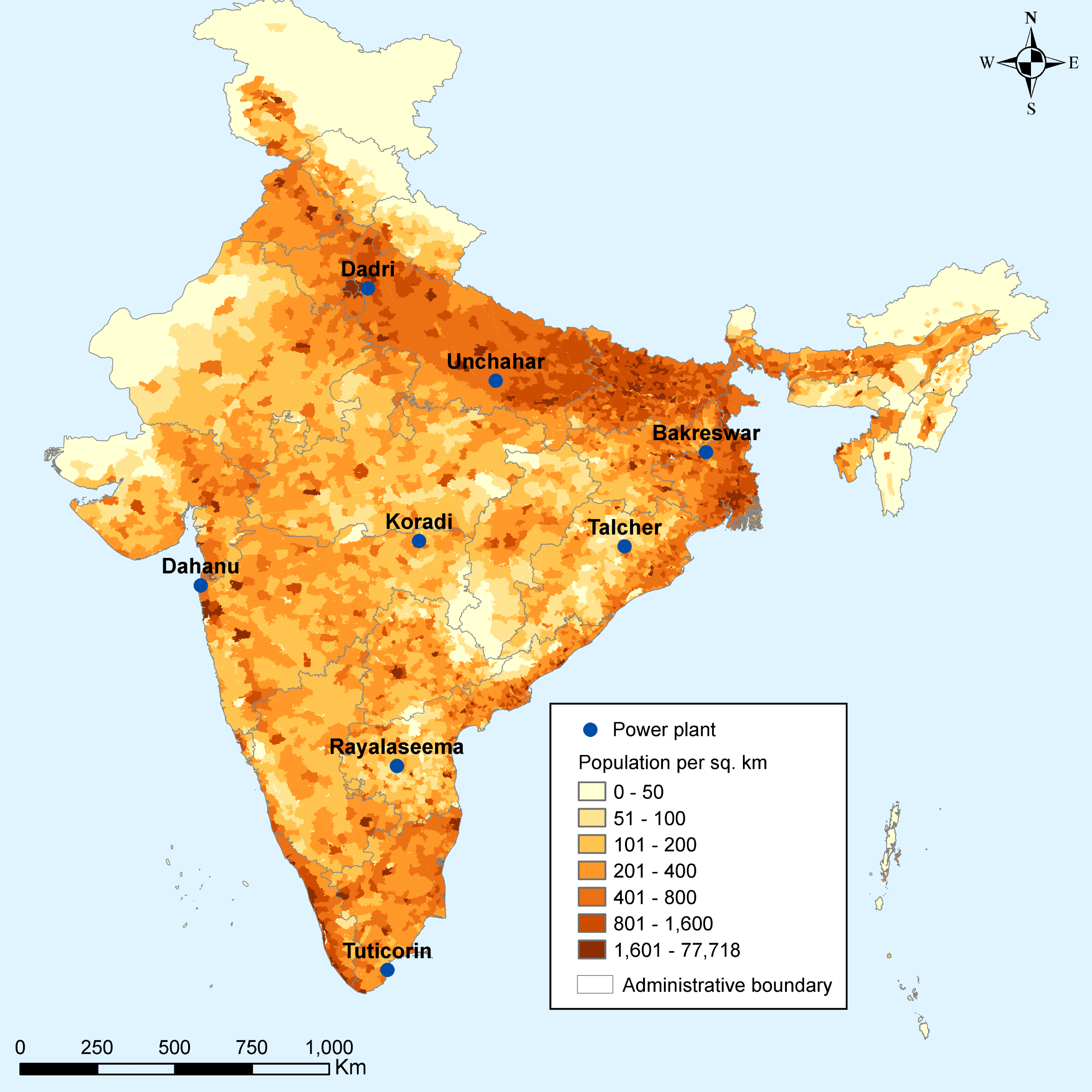
Figure 1 Locations of Model Power Plants.
Analyzing the benefits of installing a scrubber requires estimating the damages associated with the plant’s SO
![]() $_{2}$
emissions with and without an FGD. Estimating the health damages associated with SO
$_{2}$
emissions with and without an FGD. Estimating the health damages associated with SO
![]() $_{2}$
emissions involves four steps: (1) estimating the plant’s SO
$_{2}$
emissions involves four steps: (1) estimating the plant’s SO
![]() $_{2}$
emissions; (2) translating emissions into their impact on ambient air pollution; (3) estimating the effect of the plant’s impact on air pollution on human health. These steps are implemented without the scrubber, and then with the scrubber. The reduction in health impacts constitutes the health benefits of scrubbing and can be monetized (step 4), to be compared with the costs of scrubbing.
$_{2}$
emissions; (2) translating emissions into their impact on ambient air pollution; (3) estimating the effect of the plant’s impact on air pollution on human health. These steps are implemented without the scrubber, and then with the scrubber. The reduction in health impacts constitutes the health benefits of scrubbing and can be monetized (step 4), to be compared with the costs of scrubbing.
To estimate SO
![]() $_{2}$
emissions from our model unit, we assume that the unit operates at a capacity factor of 85 percent, burns coal containing 0.5 percent sulfur by weight and consumes 0.69 kg of coal per kWh of electricity generated (Cropper et al., Reference Cropper, Guttikunda, Jawahar, Malik and Partridge2017). The 85 percent capacity factor reflects the Central Electricity Authority of India’s benchmark operating conditions. Domestic coal is approximately 0.5 percent sulfur by weight (Lu et al., Reference Lu, Streets, de Foy and Krotkov2013; CSTEP, 2018).Footnote
7
Our assumptions imply that, without an FGD, the unit generates 20,442 tons of SO
$_{2}$
emissions from our model unit, we assume that the unit operates at a capacity factor of 85 percent, burns coal containing 0.5 percent sulfur by weight and consumes 0.69 kg of coal per kWh of electricity generated (Cropper et al., Reference Cropper, Guttikunda, Jawahar, Malik and Partridge2017). The 85 percent capacity factor reflects the Central Electricity Authority of India’s benchmark operating conditions. Domestic coal is approximately 0.5 percent sulfur by weight (Lu et al., Reference Lu, Streets, de Foy and Krotkov2013; CSTEP, 2018).Footnote
7
Our assumptions imply that, without an FGD, the unit generates 20,442 tons of SO
![]() $_{2}$
per year.
$_{2}$
per year.
SO
![]() $_{2}$
emissions react in the atmosphere with ammonia to form fine particles (PM
$_{2}$
emissions react in the atmosphere with ammonia to form fine particles (PM
![]() $_{2.5}$
, in the form of ammonium sulfate). Because of the health impacts of PM
$_{2.5}$
, in the form of ammonium sulfate). Because of the health impacts of PM
![]() $_{2.5}$
, we focus on this measure of ambient air quality. Translating the plant’s emissions into impacts on ambient air quality requires dispersion models that track the transport of pollutants through the atmosphere using information on weather, topography and pollutant chemistry. Dispersion models may be either process-based or reduced form (NRC, 2010). Process-based models (e.g., CAMx, CMAQ) use detailed atmospheric chemistry to simulate interactions among pollutants and gases in the atmosphere and thus account for nonlinearity in the dispersion process. Process-based models are, however, more computationally intensive than reduced-form models. Reduced-form models (e.g., CALPUFF, HYSPLIT) use simplified dispersion calculations to predict concentration changes. In this paper we use CAMx,Footnote
8
which captures the transformation of SO
$_{2.5}$
, we focus on this measure of ambient air quality. Translating the plant’s emissions into impacts on ambient air quality requires dispersion models that track the transport of pollutants through the atmosphere using information on weather, topography and pollutant chemistry. Dispersion models may be either process-based or reduced form (NRC, 2010). Process-based models (e.g., CAMx, CMAQ) use detailed atmospheric chemistry to simulate interactions among pollutants and gases in the atmosphere and thus account for nonlinearity in the dispersion process. Process-based models are, however, more computationally intensive than reduced-form models. Reduced-form models (e.g., CALPUFF, HYSPLIT) use simplified dispersion calculations to predict concentration changes. In this paper we use CAMx,Footnote
8
which captures the transformation of SO
![]() $_{2}$
into sulfate particles (PM
$_{2}$
into sulfate particles (PM
![]() $_{2.5}$
).Footnote
9
$_{2.5}$
).Footnote
9
We ran CAMx for 72 power plant locations in India. The model was run separately for each location, simulating 365 days of emissions, to calculate the increase in annual average fine particle concentrations corresponding to the model unit’s emissions.Footnote
10
We assumed a stack height of 210 meters, the minimum stack height required by law for a 500 MW generating unit. The model was run at a
![]() $0.25^{\circ }$
grid resolution (approximately
$0.25^{\circ }$
grid resolution (approximately
![]() $27~\text{km}\times 27~\text{km}$
) and combined with 2011 population data to calculate the population-weighted increase in annual average PM
$27~\text{km}\times 27~\text{km}$
) and combined with 2011 population data to calculate the population-weighted increase in annual average PM
![]() $_{2.5}$
concentrations associated with the model plant.Footnote
11
$_{2.5}$
concentrations associated with the model plant.Footnote
11
The eight locations chosen for our analysis are based on estimates of mortality due to fine particles associated with the plant’s SO
![]() $_{2}$
emissions (step 3 of the analysis). Epidemiological research has found consistent associations between premature mortality and PM
$_{2}$
emissions (step 3 of the analysis). Epidemiological research has found consistent associations between premature mortality and PM
![]() $_{2.5}$
. Pope et al. (Reference Pope III, Burnett, Thun, Calle, Krewski, Ito and Thurston2002) report significant impacts of exposure to PM
$_{2.5}$
. Pope et al. (Reference Pope III, Burnett, Thun, Calle, Krewski, Ito and Thurston2002) report significant impacts of exposure to PM
![]() $_{2.5}$
in cites in the US on all-cause, cardiopulmonary and lung cancer mortality. This work formed the basis of early studies of the global burden of air pollution (Cohen et al., Reference Cohen, Anderson, Ostro, Pandey, Krzyzanowski, Kuenzli, Gutschmidt, Pope III, Romieu, Samet, Smith, Ezzati, Lopez, Rodgers and Murray2004). More recent studies of the Global Burden of Disease (Lim et al., Reference Lim, Vos, Flaxman, Danaei, Shibuya, Adair-Rohani and AlMazroa2012; GBD 2015 Risk Factor Collaborators, 2016) use meta-analyses of epidemiological studies from several sources to quantify the impact of a wider range of PM
$_{2.5}$
in cites in the US on all-cause, cardiopulmonary and lung cancer mortality. This work formed the basis of early studies of the global burden of air pollution (Cohen et al., Reference Cohen, Anderson, Ostro, Pandey, Krzyzanowski, Kuenzli, Gutschmidt, Pope III, Romieu, Samet, Smith, Ezzati, Lopez, Rodgers and Murray2004). More recent studies of the Global Burden of Disease (Lim et al., Reference Lim, Vos, Flaxman, Danaei, Shibuya, Adair-Rohani and AlMazroa2012; GBD 2015 Risk Factor Collaborators, 2016) use meta-analyses of epidemiological studies from several sources to quantify the impact of a wider range of PM
![]() $_{2.5}$
exposures on cardiovascular and respiratory deaths, as well as premature deaths from lung cancer and acute lower respiratory infection (ALRI) (Burnett et al., Reference Burnett, Pope III, Ezzati, Olives, Lim, Mehta and Shin2014).
$_{2.5}$
exposures on cardiovascular and respiratory deaths, as well as premature deaths from lung cancer and acute lower respiratory infection (ALRI) (Burnett et al., Reference Burnett, Pope III, Ezzati, Olives, Lim, Mehta and Shin2014).
We calculate premature mortality associated with the increase in annual average PM
![]() $_{2.5}$
concentrations for each of 72 locations as the product of baseline deaths, by cause, and the fraction of premature deaths attributable to sulfates. The fraction of premature deaths attributable to sulfates for each disease is given by
$_{2.5}$
concentrations for each of 72 locations as the product of baseline deaths, by cause, and the fraction of premature deaths attributable to sulfates. The fraction of premature deaths attributable to sulfates for each disease is given by
![]() $1-\exp (\unicode[STIX]{x1D6FD}^{\ast }\unicode[STIX]{x1D6E5}C)$
, where
$1-\exp (\unicode[STIX]{x1D6FD}^{\ast }\unicode[STIX]{x1D6E5}C)$
, where
![]() $\unicode[STIX]{x1D6FD}$
is the change in the relative risk attributable to a one microgram per cubic meter change in PM
$\unicode[STIX]{x1D6FD}$
is the change in the relative risk attributable to a one microgram per cubic meter change in PM
![]() $_{2.5}$
and
$_{2.5}$
and
![]() $\unicode[STIX]{x1D6E5}C$
is the population-weighted change in ambient PM
$\unicode[STIX]{x1D6E5}C$
is the population-weighted change in ambient PM
![]() $_{2.5}$
concentrations associated with SO
$_{2.5}$
concentrations associated with SO
![]() $_{2}$
emissions from the plant. The
$_{2}$
emissions from the plant. The
![]() $\unicode[STIX]{x1D6FD}$
coefficients were calculated using the Integrated Exposure Response functions (IERs) for ischemic heart disease, stroke, lung cancer, chronic obstructive pulmonary disease (COPD), and ALRI developed by Burnett et al. (Reference Burnett, Pope III, Ezzati, Olives, Lim, Mehta and Shin2014) and reported by the Institute for Health Metrics and Evaluation (IHME).Footnote
12
For each disease, the change in relative risk (
$\unicode[STIX]{x1D6FD}$
coefficients were calculated using the Integrated Exposure Response functions (IERs) for ischemic heart disease, stroke, lung cancer, chronic obstructive pulmonary disease (COPD), and ALRI developed by Burnett et al. (Reference Burnett, Pope III, Ezzati, Olives, Lim, Mehta and Shin2014) and reported by the Institute for Health Metrics and Evaluation (IHME).Footnote
12
For each disease, the change in relative risk (
![]() $\unicode[STIX]{x1D6FD}$
) was evaluated at the population-weighted annual average exposures for India used in the 2010 Global Burden of Disease (Brauer et al., Reference Brauer, Amann, Burnett, Cohen, Dentener, Ezzati, Henderson, Krzyzanowski, Martin, Van Dingenen, van Donkelaar and Thurston2012).Footnote
13
Baseline deaths by age and cause were obtained from the IHME.Footnote
14
$\unicode[STIX]{x1D6FD}$
) was evaluated at the population-weighted annual average exposures for India used in the 2010 Global Burden of Disease (Brauer et al., Reference Brauer, Amann, Burnett, Cohen, Dentener, Ezzati, Henderson, Krzyzanowski, Martin, Van Dingenen, van Donkelaar and Thurston2012).Footnote
13
Baseline deaths by age and cause were obtained from the IHME.Footnote
14
We ranked the 72 locations by premature deaths per ton of SO
![]() $_{2}$
emitted and selected eight of the locations to conduct the present analysis. Plant locations were chosen to represent a range of SO
$_{2}$
emitted and selected eight of the locations to conduct the present analysis. Plant locations were chosen to represent a range of SO
![]() $_{2}$
impacts as well as geographic locations throughout the country (see Figure 1). Table 1 lists the eight plant locations and the premature deaths per ton of SO
$_{2}$
impacts as well as geographic locations throughout the country (see Figure 1). Table 1 lists the eight plant locations and the premature deaths per ton of SO
![]() $_{2}$
emitted. Table 1 also lists estimates of the annual premature deaths associated with SO
$_{2}$
emitted. Table 1 also lists estimates of the annual premature deaths associated with SO
![]() $_{2}$
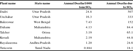
emissions from the model 500 MW electricity generating unit installed at each location. Two locations, Dahanu and Tuticorin, are on the coast and can therefore accommodate a seawater FGD. Baseline premature deaths range from 18 to over 500 per year. Deaths are highly correlated with population density (see Figure 1), but also reflect meteorological conditions. Premature deaths per ton are highest at the three plant locations in the north of India: Dadri, Unchahar and Bakreswar.
$_{2}$
emissions from the model 500 MW electricity generating unit installed at each location. Two locations, Dahanu and Tuticorin, are on the coast and can therefore accommodate a seawater FGD. Baseline premature deaths range from 18 to over 500 per year. Deaths are highly correlated with population density (see Figure 1), but also reflect meteorological conditions. Premature deaths per ton are highest at the three plant locations in the north of India: Dadri, Unchahar and Bakreswar.
Table 1 Locations and impacts of model plants.
3 Benefits analysis
SO
![]() $_{2}$
emissions react in the atmosphere with ammonia to form fine particles (PM
$_{2}$
emissions react in the atmosphere with ammonia to form fine particles (PM
![]() $_{2.5}$
, in the form of ammonium sulfate) and with water to form sulfuric acid (acid rain). Particulate matter has been linked to heart and lung disease, as described above, but also to impacts on brain development and functioning (Brockmeyer & D’Angiulli, Reference Brockmeyer and D’Angiulli2016; Landrigan et al., Reference Landrigan, Fuller, Acosta, Adeyi, Arnold, Baldé and Bertollini2017). It also impairs visibility. Acidic deposition can reduce soil quality, impair timber growth and harm freshwater ecosystems (US EPA, 2011). In estimating the benefits of reducing SO
$_{2.5}$
, in the form of ammonium sulfate) and with water to form sulfuric acid (acid rain). Particulate matter has been linked to heart and lung disease, as described above, but also to impacts on brain development and functioning (Brockmeyer & D’Angiulli, Reference Brockmeyer and D’Angiulli2016; Landrigan et al., Reference Landrigan, Fuller, Acosta, Adeyi, Arnold, Baldé and Bertollini2017). It also impairs visibility. Acidic deposition can reduce soil quality, impair timber growth and harm freshwater ecosystems (US EPA, 2011). In estimating the benefits of reducing SO
![]() $_{2}$
emissions, we focus on health benefits, specifically, on the mortality benefits estimated using the IERs described above.Footnote
15
We do not quantify either the benefits of reduced morbidity associated with fine particles or the benefits of reduced acid deposition; hence our benefit estimates significantly underestimate the benefits of scrubbing SO
$_{2}$
emissions, we focus on health benefits, specifically, on the mortality benefits estimated using the IERs described above.Footnote
15
We do not quantify either the benefits of reduced morbidity associated with fine particles or the benefits of reduced acid deposition; hence our benefit estimates significantly underestimate the benefits of scrubbing SO
![]() $_{2}$
.
$_{2}$
.
To calculate premature deaths avoided, we assume that installation of a scrubber will remove 90 percent of sulfur dioxide emissions.Footnote
16
Due to the linearity of sulfate formation and the approximate linearity of concentration-response for a small change in concentrations, this reduction in emissions implies a 90 percent reduction in premature deaths attributable to SO
![]() $_{2}$
emissions. An important question is the period over which this reduction would occur. Apte et al. (Reference Apte, Marshall, Cohen and Brauer2015) assume no lag between emissions reductions and the associated reduction in premature deaths. The US Environmental Protection Agency (EPA) (2011) assumes that 80 percent of the reduction in PM
$_{2}$
emissions. An important question is the period over which this reduction would occur. Apte et al. (Reference Apte, Marshall, Cohen and Brauer2015) assume no lag between emissions reductions and the associated reduction in premature deaths. The US Environmental Protection Agency (EPA) (2011) assumes that 80 percent of the reduction in PM
![]() $_{2.5}$
mortality is achieved within five years of the reduction in emissions, although alternate lag structures have been considered (EPA, 2013). A conservative approach is to assume that the scrubber reduces 72 percent of premature deaths in each year of its 20-year operation. This is equivalent to assuming a lag structure that reduces the present value of premature deaths avoided to 0.8 times total premature deaths avoided.Footnote
17
We calculate premature deaths avoided in the base year
$_{2.5}$
mortality is achieved within five years of the reduction in emissions, although alternate lag structures have been considered (EPA, 2013). A conservative approach is to assume that the scrubber reduces 72 percent of premature deaths in each year of its 20-year operation. This is equivalent to assuming a lag structure that reduces the present value of premature deaths avoided to 0.8 times total premature deaths avoided.Footnote
17
We calculate premature deaths avoided in the base year
![]() $(\text{Deaths Avoided}_{0})$
as 0.72 (
$(\text{Deaths Avoided}_{0})$
as 0.72 (
![]() $=$
0.9
$=$
0.9
![]() $\times$
0.8) of the baseline deaths attributable to the model plant (see Table 1). We assume that premature deaths avoided increase in proportion to the projected rate of population increase (
$\times$
0.8) of the baseline deaths attributable to the model plant (see Table 1). We assume that premature deaths avoided increase in proportion to the projected rate of population increase (
![]() $g_{l}$
) which we assume to equal 0.94 percent per year (Population Reference Bureau, 2007).
$g_{l}$
) which we assume to equal 0.94 percent per year (Population Reference Bureau, 2007).
Ideally, we would like to value premature deaths avoided using studies of mortality risk reductions conducted in India. The value per statistical life (VSL) reported in these studies, however, varies widely. Bhattacharya et al. (Reference Bhattacharya, Alberini and Cropper2007) report a preferred VSL estimate of Rs. 1.3 million (2006 Rs.) based on a stated preference study of Delhi residents. Madheswaran (Reference Madheswaran2007) estimates the VSL based on a compensating wage study of workers in Calcutta and Mumbai to be approximately Rs. 15 million. Shanmugam (Reference Shanmugam2001) reports a much higher value (Rs. 56 million) using 1990 data on workers in Madras.
We therefore value each death avoided using values transferred from high income countries, following reference case protocols developed by Robinson et al. (Reference Robinson, Hammitt and O’Keeffe2018). The three VSL values, in 2015 International (PPP) dollars, are $969,600 (160 times per capita GNI), $606,000 (100 times per capita GNI) and $318,287 (53 times per capita GNI, extrapolated from the US VSL using an elasticity of 1.5). In the text we present all costs and benefits in USD at market exchange rates.Footnote 18 The corresponding transferred VSLs in 2015$ are $256,000, $160,000 and $84,036.
We assume that the transferred VSL in the base year, VSL
![]() $_{0}$
, grows at a rate that depends on the rate of growth in per capita income in India (
$_{0}$
, grows at a rate that depends on the rate of growth in per capita income in India (
![]() $g_{p}$
), and the income elasticity of the VSL (
$g_{p}$
), and the income elasticity of the VSL (
![]() $\unicode[STIX]{x1D700}$
). Specifically,
$\unicode[STIX]{x1D700}$
). Specifically,
![]() $\text{VSL}_{t}=\text{VSL}_{0}[(1+g_{p})^{t}]^{\unicode[STIX]{x1D700}}$
. We estimate
$\text{VSL}_{t}=\text{VSL}_{0}[(1+g_{p})^{t}]^{\unicode[STIX]{x1D700}}$
. We estimate
![]() $g_{p}$
to be 6.3 percent per year.Footnote
19
We use an
$g_{p}$
to be 6.3 percent per year.Footnote
19
We use an
![]() $\unicode[STIX]{x1D700}=1$
when the VSL is transferred using an income elasticity of 1 (i.e., using the first two transfer approaches), and
$\unicode[STIX]{x1D700}=1$
when the VSL is transferred using an income elasticity of 1 (i.e., using the first two transfer approaches), and
![]() $\unicode[STIX]{x1D700}=1.5$
when the VSL is transferred from the US using an income elasticity of 1.5. The present discounted value of the mortality benefits from scrubbing is given by equation (1), where
$\unicode[STIX]{x1D700}=1.5$
when the VSL is transferred from the US using an income elasticity of 1.5. The present discounted value of the mortality benefits from scrubbing is given by equation (1), where
![]() $r$
is the rate at which benefits are discounted. We use the reference case value of
$r$
is the rate at which benefits are discounted. We use the reference case value of
![]() $r=0.03$
(Wilkinson et al., Reference Wilkinson, Sculpher, Claxton, Revill, Briggs, Cairns, Teerawattananon, Asfaw, Lopert, Culyer and Walker2016), but also use a higher rate of
$r=0.03$
(Wilkinson et al., Reference Wilkinson, Sculpher, Claxton, Revill, Briggs, Cairns, Teerawattananon, Asfaw, Lopert, Culyer and Walker2016), but also use a higher rate of
![]() $r=0.08$
. The latter is consistent with the rate of return on government bonds in India, and also reflects the higher rate of income growth in the country. As a sensitivity analysis we use a value of
$r=0.08$
. The latter is consistent with the rate of return on government bonds in India, and also reflects the higher rate of income growth in the country. As a sensitivity analysis we use a value of
![]() $r=0.12$
, or two times the near-term growth rate (motivated by the Ramsey rule).
$r=0.12$
, or two times the near-term growth rate (motivated by the Ramsey rule).
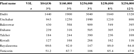
Table 2 shows the presented discounted value of mortality benefits, computed using alternate values of VSL
![]() $_{0}$
and alternate discount rates. The present value of benefits ranges from $3.04 billion (2015$) to $108 million using the highest VSL and
$_{0}$
and alternate discount rates. The present value of benefits ranges from $3.04 billion (2015$) to $108 million using the highest VSL and
![]() $r=0.03$
. Using the conservative value of $84,036 and
$r=0.03$
. Using the conservative value of $84,036 and
![]() $r=0.03$
, they range from $1.44 billion to $51.2 million. With a VSL
$r=0.03$
, they range from $1.44 billion to $51.2 million. With a VSL
![]() $_{0}$
of $256,000, raising the discount rate from 3 percent to 8 percent lowers the present value of benefits by 40 percent; raising it to 12 percent lowers the present value of benefits by 57 percent.
$_{0}$
of $256,000, raising the discount rate from 3 percent to 8 percent lowers the present value of benefits by 40 percent; raising it to 12 percent lowers the present value of benefits by 57 percent.
Table 2 Present value of mortality benefits of an FGD in millions (2015$).
An alternate approach, which we do not follow, is to use the value per statistical life year (VSLY) multiplied by the expected number of life years gained. The VSLY approach is widely used in Europe, although its theoretical foundations have been criticized (Hammitt, Reference Hammitt2007). On average, each expected death averted leads to a gain in 25.5 life years when a scrubber is installed. If calculated using the recommendations in Robinson et al. (Reference Robinson, Hammitt and O’Keeffe2018), the VSLY is estimated by dividing the VSL by the remaining life expectancy of an adult of average age. The remaining life expectancy of a 44-year old adult in India is approximately 34.4 years.Footnote 20 Multiplying the average number of life years saved by the VSLY would, therefore, reduce the present value of mortality benefits in Table 2 by about 25 percent.
4 Analysis of costs
An FGD is an end-of-pipe technology that removes SO
![]() $_{2}$
from combustion gases before they exit the smokestack. Flue gases are treated with an alkaline substance that reacts with the acidic SO
$_{2}$
from combustion gases before they exit the smokestack. Flue gases are treated with an alkaline substance that reacts with the acidic SO
![]() $_{2}$
to form a by-product that is removed before flue gases are emitted. In a wet limestone FGD (wFGD), gases are treated with limestone slurry, which is sprayed on the gas in an absorber unit. Gypsum, which can be sold commercially, is produced as a by-product. Another rapidly expanding technology is seawater FGDs (swFGDs). These units use the alkalinity of seawater to remove SO
$_{2}$
to form a by-product that is removed before flue gases are emitted. In a wet limestone FGD (wFGD), gases are treated with limestone slurry, which is sprayed on the gas in an absorber unit. Gypsum, which can be sold commercially, is produced as a by-product. Another rapidly expanding technology is seawater FGDs (swFGDs). These units use the alkalinity of seawater to remove SO
![]() $_{2}$
from the flue gases. The by-product is water, which is treated and discharged back into the sea. FGDs are capable of reducing SO
$_{2}$
from the flue gases. The by-product is water, which is treated and discharged back into the sea. FGDs are capable of reducing SO
![]() $_{2}$
emissions up to 95 percent, depending on the technology used.Footnote
21
$_{2}$
emissions up to 95 percent, depending on the technology used.Footnote
21
Both scrubber technologies are in use in India. The Indian Supreme Court required the installation of an FGD at the Dahanu plant in Maharashtra. FGDs are also in operation at the Trombay and Udupi plants. FGDs have also been commissioned at several other plants, including Dadri and Koradi.Footnote 22 Both Dahanu and Trombay have swFGDs. Seawater FGDs have lower capital and variable costs than wet limestone FGDs, but they can be installed only in coastal areas. We assume that all FGDs installed at plants in coastal areas are swFGDs and that wet limestone FGDs are installed at all other locations.
The costs of FGD adoption include the capital costs of FGD installation and annual operating costs. The capital costs of installation include one-time equipment purchase and the costs of setting up the FGD unit and connecting it to the boiler and flue stack. Based on the type of FGD, additional equipment, such as a limestone storage unit, mill and gypsum handling unit in the case of a wet limestone FGD, or water treatment in the case of a sea water FGD, also needs to be purchased. Operating costs include periodic maintenance and labor to operate and maintain the FGD and accompanying equipment, the purchase of reagent (limestone in the case of wFGD) and by-product handling and disposal. Auxiliary consumption of electricity by the FGD is also a part of the variable costs of operation.
Table 3 Operating characteristics for cost calculations: baseline assumptions.
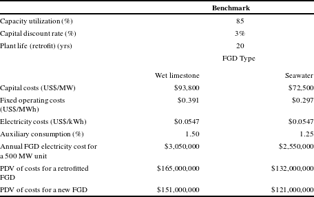
Table 3 shows the assumptions used to construct the cost estimates. Capital costs for a wFGD are based on costs for installing FGDs on each of two 490 MW units proposed for the Dadri plant.Footnote 23 Capital costs for a swFGD are based on the FGD installed on two 250 MW units at the Dahanu plant (MERC, 2009). These yield a capital cost of US$93,800/MW (2015$) for a wFGD and a cost of US$72,500/MW (2015$) for a swFGD. The greater costs for a limestone FGD reflect the expenditure on reagent handling and by-product disposal facilities. In contrast, a swFGD discharges the water back into the sea and does not require as much capital investment. We increase both figures by 30 percent to reflect additional retrofitting costs. The operating and maintenance costs are based on those at the Dahanu plant (MERC, 2009). We assume that these are 30 percent higher for a wFGD (Malik, Reference Malik2013).Footnote 24
The present value of the cost of retrofitting a scrubber with a life of 20 years is given by equation (2), where
![]() $d$
represents the rate of increase in the costs of operating the scrubber.
$d$
represents the rate of increase in the costs of operating the scrubber.
Since the FGD operation and maintenance cost information for plants in India is limited, we assume that the operation and maintenance costs in India grow at the same rate as in the U.S.Footnote
25
Using the average annual operation and maintenance cost information from the U.S. Energy Information Administration (2016), the value of
![]() $d$
was determined by calculating the compound rate of growth of the operation and maintenance cost from 2005 to 2015. This value was calculated to be 4 percent. Using a discount rate of
$d$
was determined by calculating the compound rate of growth of the operation and maintenance cost from 2005 to 2015. This value was calculated to be 4 percent. Using a discount rate of
![]() $r=0.03$
yields a present value of $165 million (2015$) for the costs of retrofitting a wFGD and $132 million (2015$) for a swFGD. The present value of costs falls to $127 million (wFGD) and $101 million (swFGD) using
$r=0.03$
yields a present value of $165 million (2015$) for the costs of retrofitting a wFGD and $132 million (2015$) for a swFGD. The present value of costs falls to $127 million (wFGD) and $101 million (swFGD) using
![]() $r=0.08$
.
$r=0.08$
.
5 The net benefits of retrofitting an FGD
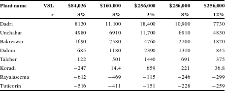
Table 4 shows the net mortality benefits from retrofitting a model power plant at eight locations in Figure 1. We assume that a swFGD is installed at the Dahanu and Tuticorin locations and a wFGD at the other six locations. Recall that the benefits computed here are a lower bound – they reflect the value of avoided mortality only and ignore the morbidity, amenity and ecosystem benefits provided by reducing SO
![]() $_{2}$
emissions. Using a VSL
$_{2}$
emissions. Using a VSL
![]() $_{0}$
equal to 100 times per capita income ($160,000), the scrubber passes the benefit-cost test based solely on mortality benefits at all but the two least-densely populated locations. At a VSL
$_{0}$
equal to 100 times per capita income ($160,000), the scrubber passes the benefit-cost test based solely on mortality benefits at all but the two least-densely populated locations. At a VSL
![]() $_{0}$
of $84,036 (53 times per capita income), the scrubber passes the benefit-cost test at five locations, based solely on mortality benefits.
$_{0}$
of $84,036 (53 times per capita income), the scrubber passes the benefit-cost test at five locations, based solely on mortality benefits.
Table 4 Net benefits from scrubbing in millions (2015$).
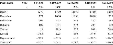
Whether an FGD retrofit passes the benefit-cost test based solely on health benefits depends on the VSL used and also on the magnitude of morbidity and other benefits, which we do not quantify. Studies suggest that the morbidity costs of pollution-related disease may conservatively increase health costs by 10–70% (Narain & Sall, Reference Narain and Sall2016; Hunt et al., Reference Hunt, Ferguson, Hurley and Searl2016). Individual country studies have found morbidity costs as a percent of mortality costs to be: 25% for Colombia (Golub et al., Reference Golub, Klytchnikova, Sanchez-Martinez and Belausteguigoitia2014), 22–78% for China (World Bank, 2007) and 78% for Nicaragua (Kemper, Reference Kemper2013). Thus the numbers in Table 4 should not be interpreted as determining whether a scrubber yields net benefits at each of the eight locations. We do, however, believe that morbidity benefits will be proportional to reductions in population-weighted concentrations of PM
![]() $_{2.5}$
and, hence, that the numbers in Table 4 can serve as a guide to prioritizing the installation of FGDs (i.e., they provide an accurate ranking of eight sites based on health benefits).
$_{2.5}$
and, hence, that the numbers in Table 4 can serve as a guide to prioritizing the installation of FGDs (i.e., they provide an accurate ranking of eight sites based on health benefits).
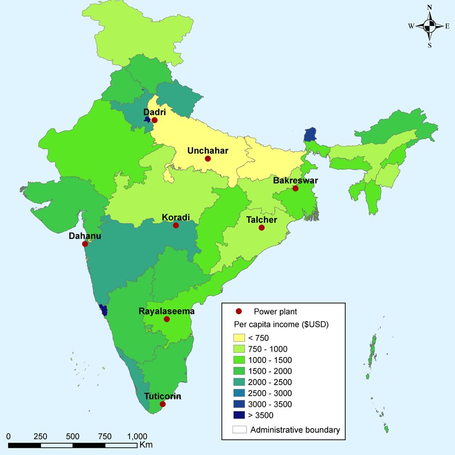
The net benefits of retrofitting the model unit based on avoided mortality are clearly greatest in the densely populated north of India. These are also some of the poorest areas in India. Figure 2 shows eight locations studied on a map of per capita GDP by state, measured for the 2014–15 fiscal year.Footnote 26 The Dadri and Unchahar plants are located in Uttar Pradesh, one of the poorest states in India, and most of the population exposed to the Bakreswar plant lives in Bihar – the poorest state in India – as well as Jharkhand and West Bengal.

Figure 2 Indian States and Union Territories by GDP per Capita (2017$).
Because the VSL used in this analysis has been transferred to India based on national per capita income, it is natural to ask whether the VSL should also vary with the per capita income of the states in which benefits are received. Such an approach would better reflect the ability of the population to allocate their resources between achieving these risk reductions and paying for other goods and services. However, we follow the practice in OECD counties of applying the same VSL to all persons within the same country; hence we do not allow the VSL to vary by state.
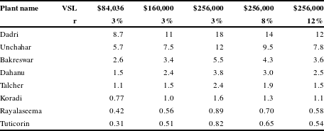
Because benefits and costs in our analysis are well-defined, we also present benefit-cost ratios (Table 5). These results mirror Table 4 – benefit-cost ratios exceed one when net benefits are positive – but are easier to comprehend and may aid in prioritizing locations where installing FGDs would yield the greatest net benefits. We note, however, that a benefit-cost ratio below one should not be interpreted as indicating that scrubbing does not yield net benefits: our benefits estimates exclude the value of avoided morbidity, as well as impacts on ecosystems and the aesthetic value of clean air. The benefit-cost ratio and the magnitude of net benefits are, however, likely to provide a useful ranking of locations in terms of net health benefits. Morbidity benefits will increase in proportion to the reduction in population-weighted PM
![]() $_{2.5}$
concentrations and in proportion to the size of the exposed population, which are positively correlated with mortality benefits.
$_{2.5}$
concentrations and in proportion to the size of the exposed population, which are positively correlated with mortality benefits.
Table 5 Benefit/cost ratios for FGD retrofits.
6 Conclusion
This paper has two objectives. One is to demonstrate the feasibility of conducting a benefit-cost analysis of air pollution control measures in a low- or middle-income country (LMIC) setting and to illustrate the sensitivity of the results to key parameters. The second is to provide information that could help to prioritize the installation of scrubbers at coal-fired power plants in India.
Estimating the benefits of a project that reduces stationary source air emissions requires (1) calculating emissions before and after the project, (2) translating the change in emissions into a change in geo-referenced ambient concentrations, (3) estimating impacts on health and other endpoints using concentration-response functions and (4) valuing these endpoints. There are uncertainties in each step, some of which we have dealt with through sensitivity analysis and others of which we have ignored. Regarding the first step, our results should be viewed as conditional on annual SO
![]() $_{2}$
emissions of 20,000 tons. Given the approximate linearity of results in steps 2 and 3 (for small changes in emissions), the results can be scaled according to differences in emission estimates.
$_{2}$
emissions of 20,000 tons. Given the approximate linearity of results in steps 2 and 3 (for small changes in emissions), the results can be scaled according to differences in emission estimates.
It is more difficult to assess the accuracy of our projections of the impact of SO
![]() $_{2}$
emissions on ambient PM
$_{2}$
emissions on ambient PM
![]() $_{2.5}$
(step 2), as well as the accuracy of our mortality projections (step 3). There have been assessments of the performance of CAMx in North America and Europe that compare the model’s projections with readings at monitoring stations and with the results of other modeling platforms (Ferreira et al., Reference Ferreira, Rodriguez, Monteiro, Miranda, Dios, Souto, Yarwood, Nopmongcol and Borrego2012; Nopmongcol et al., Reference Nopmongcol, Koo, Tai, Jung, Piyachaturawat, Emery, Yarwood, Pirovano, Mitsakou and Kallos2012; Pirovano et al., Reference Pirovano, Balzarini, Bessagnet, Emery, Kallos, Meleux, Mitsakou, Nopmongcol, Riva and Yarwood2012; Tesche et al., Reference Tesche, Morris, Tonnesen, McNally, Boylan and Brewer2006), but none that we could find for India. The concentration-response functions we have used to estimate the mortality impacts of PM
$_{2.5}$
(step 2), as well as the accuracy of our mortality projections (step 3). There have been assessments of the performance of CAMx in North America and Europe that compare the model’s projections with readings at monitoring stations and with the results of other modeling platforms (Ferreira et al., Reference Ferreira, Rodriguez, Monteiro, Miranda, Dios, Souto, Yarwood, Nopmongcol and Borrego2012; Nopmongcol et al., Reference Nopmongcol, Koo, Tai, Jung, Piyachaturawat, Emery, Yarwood, Pirovano, Mitsakou and Kallos2012; Pirovano et al., Reference Pirovano, Balzarini, Bessagnet, Emery, Kallos, Meleux, Mitsakou, Nopmongcol, Riva and Yarwood2012; Tesche et al., Reference Tesche, Morris, Tonnesen, McNally, Boylan and Brewer2006), but none that we could find for India. The concentration-response functions we have used to estimate the mortality impacts of PM
![]() $_{2.5}$
have been updated by the Global Burden of Disease (GBD) team (see Ostro et al., Reference Ostro, Spadaro, Gumy, Mudu, Awe, Forastiere and Peters2018 for a summary) and a recent reanalysis of prospective cohort data (Burnett et al., Reference Burnett, Chen, Szyszkowicz, Fann, Hubbell, Pope and Apte2018) suggests much larger impacts of fine particles on mortality than those embodied in our analyses. It is also the case that we use national death rates to estimate mortality impacts, rather than state- (or district-) specific ones, which introduces additional error into the analysis.
$_{2.5}$
have been updated by the Global Burden of Disease (GBD) team (see Ostro et al., Reference Ostro, Spadaro, Gumy, Mudu, Awe, Forastiere and Peters2018 for a summary) and a recent reanalysis of prospective cohort data (Burnett et al., Reference Burnett, Chen, Szyszkowicz, Fann, Hubbell, Pope and Apte2018) suggests much larger impacts of fine particles on mortality than those embodied in our analyses. It is also the case that we use national death rates to estimate mortality impacts, rather than state- (or district-) specific ones, which introduces additional error into the analysis.
Regarding the valuation of mortality impacts (step 4) we have used sensitivity analysis to examine the impact of alternate valuation assumptions, specifically, using different approaches to transfer the VSL from other countries to India and using different discount rates. As Tables 2 and 4 demonstrate, the magnitude of the present value of mortality benefits is very sensitive to both the VSL and the discount rate, as is the present value of mortality benefits net of scrubbing costs. We emphasize, however, that the ranking of locations based on net mortality benefits is unaffected by the choice of the VSLs or discount rates that we have considered. Because the morbidity benefits of scrubbing should be positively correlated with deaths avoided, this ranking should also be robust to the inclusion of morbidity benefits, which we have not quantified. Thus, our analysis can provide useful information for prioritizing locations for retrofitting plants with FGDs based on health considerations.
We emphasize, however, that in locations where the net mortality benefits of scrubbing are negative (as reported in Table 4) the total net benefits of scrubbing are not necessarily negative. We have not quantified (or monetized) the morbidity benefits of reduced PM
![]() $_{2.5}$
concentrations, nor have we examined ecosystem or aesthetic benefits. These remain a subject for future research.
$_{2.5}$
concentrations, nor have we examined ecosystem or aesthetic benefits. These remain a subject for future research.
Acknowledgments
We thank Johannes Urpelainen and two anonymous reviewers for helpful comments and suggestions on earlier drafts. This paper was prepared as part of the “Guidelines for Benefit-Cost Analysis” project at the Harvard T.H. Chan School of Public Health, with support from the Bill & Melinda Gates Foundation [OPP1160057]. The views expressed in this paper are those of the authors and do not necessarily reflect the views of these organizations, the World Bank or the project team. For more information, see https://sites.sph.harvard.edu/bcaguidelines/.
Appendix A
Table A1 Present value of mortality benefits of an FGD in millions (2015 PPP$).
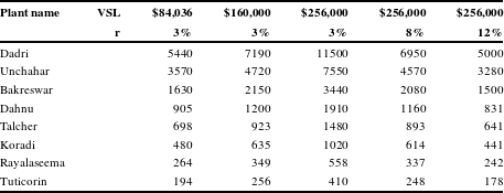
Table A2 Net benefits from scrubbing in millions (2015 PPP$).
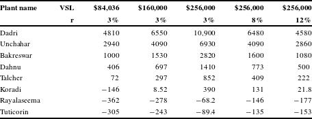
Table A3 Present value of mortality benefits of an FGD in crores (2015 Rs.).

Table A4 Operating characteristics for cost calculations: baseline assumptions.

Table A5 Net Benefits from Scrubbing in Crores (2015 Rs.).
