


1. Introduction
Food labels can convey several credence attributes related to food production practices (e.g., origin, environmental certifications, etc.), striving to make information more available and transparent for consumers and potentially improving the market share of a product (Bonroy and Constantatos, Reference Bonroy and Constantatos2014). Product adoption and ultimate success depend on consumers’ acceptance, perceptions, and willingness to pay (WTP) for what the labels convey (Caswell and Mojduszka, Reference Caswell and Mojduszka1996). With an increasingly competitive and global marketplace, suppliers may find it profitable to adopt certain labeling strategies to differentiate their food products. By evaluating a diverse sample of U.S. consumers and their assessments of selected seafood labels, this study contributes to the literature by investigating whether certain labeling schemes, some of which have not been examined previously, receive significant consumer support.
Seafood is the most widely traded food commodity in the world, with most consumption in developed countries supplied from developing nations (Asche et al., Reference Asche, Bellemare, Roheim, Smith and Tveteras2015; Jacquet et al., Reference Jacquet, Pauly, Ainley, Holt, Dayton and Jackson2010). To illustrate, by value approximately 80% of U.S. seafood consumption is imported (Lowther and Liddel, Reference Lowther and Liddel2015). Total U.S. import values of fishery products were $35.9 billion in 2014, an increase of 8% over the previous year (Lowther and Liddel, Reference Lowther and Liddel2015). Considering this extent of trade and competition, there is also a strong incentive to differentiate one’s product. Labeling specific characteristics and segmenting the market is a popular strategy to accomplish this goal.
Using shrimp as the focus product, the present study contributes to the literature by investigating consumers’ preferences for several seafood labeling options, including some that, to the best of our knowledge, have not been previously examined. Specifically, the following labels are evaluated: Fresh (Never Frozen) or Previously Frozen (representing the “product form”), Best Aquaculture Practices (BAP), Kentucky Proud or Certified South Carolina Seafood (representing “local”), a hypothetical “Product of Community-Supported Fishery” (CSF), and Homegrown by Heroes (HBH). No study has evaluated how HBH or a CSF-derived product may affect consumer choices, and little research has been devoted to aquaculture ecolabels like BAP. Preferences are assessed through WTP estimates. Furthermore, various consumer profiles are generated from the choice model results suggesting vastly different WTP according to consumer characteristics.
Our empirical analysis focuses on consumers’ preferences for farm-raised shrimp among Kentucky and South Carolina residents. A number of reasons explain these specific choices. Shrimp is of interest from a demand perspective, with consumption higher than any other seafood in the United States (Lowther and Liddel, Reference Lowther and Liddel2015). Second, Kentucky and South Carolina are both southeastern states with a significant number of shrimp farms. The U.S. Department of Agriculture, National Agricultural Statistics Service’s (USDA-NASS) most recent Census of Aquaculture discloses an array of seafood farms for South Carolina, with shellfishFootnote 1 such as shrimp providing most of the state’s aquaculture production (USDA-NASS, 2014). Freshwater aquaculture is notable for Kentucky, with the inland state having the most freshwater shrimp farms at the time of the census (USDA-NASS, 2014). To make the products in the two states more comparable, this analysis does not distinguish between freshwater and saltwater shrimp, and respondents were told to evaluate freshwater shrimp. Third, Kentucky and South Carolina are among several states that have devoted significant research to the viability and production of shrimp aquaculture. Last, with Kentucky having no direct access to the sea and South Carolina located on the coast, these contrasting locations also provide a respectable foreground for studying demand.
2. Background
Evaluating recent perceptions of shrimp products can disclose current and future trends in consumption, as market research is important in assessing consumer preferences. Although the literature pertaining to seafood is not as extensive as other food products, research devoted to consumer perceptions and attitudes has progressed in the past 25 years (e.g., Anderson and Bettencourt, Reference Anderson and Bettencourt1993; Charles and Boude, Reference Charles and Boude2001; Davidson et al., Reference Davidson, Pan, Hu and Poerwanto2012; Hanson, Herrmann, and Dunn, Reference Hanson, Herrmann and Dunn1995; Holland and Wessells, Reference Holland and Wessells1998; Jaffry et al., Reference Jaffry, Pickering, Ghulam, Whitmarsh and Wattage2004; Johnston et al., Reference Johnston, Wessells, Donath and Asche2001; O’Dierno et al., Reference O’Dierno, Govindasamy, Puduri, Myers and Islam2006; Quagrainie, Hart, and Brown, Reference Quagrainie, Hart and Brown2008; Ratliff, Vassalos, and Hu, Reference Ratliff, Vassalos and Hu2018; Roheim, Sudhakaran, and Durham, Reference Roheim, Sudhakaran and Durham2012; Rudd, Pelletier, and Tyedmers, Reference Rudd, Pelletier and Tyedmers2011; Wessells, Kline, and Anderson, Reference Wessells, Kline and Anderson1996; Whitmarsh and Palmieri, Reference Whitmarsh and Palmieri2009). Carlucci et al. (Reference Carlucci, Nocella, Devitiis, Viscecchia, Bimbo and Nardone2015) provide a detailed literature review of recent seafood preference studies in the United States and Europe. The research highlights that quality, safety, and price are important factors for consumers’ seafood purchasing decisions. However, when compared with consumers of other animal proteins, seafood consumers may have unique preferences. For instance, although research indicates that consumers will pay premiums for U.S. meat products (e.g., Lim et al., Reference Lim, Hu, Maynard and Goddard2013; Loureiro and Umberger, Reference Loureiro and Umberger2003), this has not always been the case for seafood. Jaffry et al. (Reference Jaffry, Pickering, Ghulam, Whitmarsh and Wattage2004) found that consumers prefer domestically caught to imported seafood for all the products they examined. However, Kuchler, Krissoff, and Harvey (Reference Kuchler, Krissoff and Harvey2010) found no statistically significant impact of country-of-origin labeling on U.S. household seafood consumption. Furthermore, Poerwanto (Reference Poerwanto2011) found strong consumer heterogeneity in participants’ preference for “previously frozen” and “never frozen” seafood, and Davidson et al. (Reference Davidson, Pan, Hu and Poerwanto2012) also supported that view. The aforementioned discussion indicates the need for further research related to consumer preferences for seafood products, assessing both “traditional” (i.e., fresh vs. frozen) and emerging credence attributes.
Following the release of the National Ocean and Atmospheric Administration’s Aquaculture Policy in June 2011, sustainable aquaculture has been strongly and globally advocated (Aquaculture Stewardship Council, 2016). The BAP is one organization certifying aquaculture production on an international scale. BAP defines the following elements as most important to responsible aquaculture: environmental responsibility, social responsibility, food safety, animal welfare, and traceability (Best Aquaculture Practices Certification, 2016). Through certifying finfish, crustaceans, and mussels, the third-party certification system outlines the elements of responsible aquaculture. BAP’s ecolabel appears on frozen and prepared seafood packages. Keeping in mind that aquaculture is pivotal to increasing seafood supply for food security, the Global Aquaculture Alliance (GAA) advocates responsible and sustainable aquaculture by working with nongovernmental organizations, industry, governments, and academia to meet these challenges (GAA, 2016). As of 2016, BAP certified 40 operations in the United States, of which 12 processed shrimp products (BAP, 2016). However, none originated specifically from Kentucky or South Carolina.
Food systems focusing on direct marketing (e.g., farmers’ markets, community-supported agriculture [CSA], etc.) have sprung up across the United States as states’ agriculture departments promote “local” producers’ products (i.e., Kentucky State Proud, Certified South Carolina Seafood, etc.; Low et al., Reference Low, Adalja, Beaulieu, Key, Martinez, Melton and Perez2015). “Local” food products are intended to represent transparency, traceability, and short supply chains (Marsden, Banks, and Bristow, Reference Marsden, Banks and Bristow2000). Similarly, preference for origin labeling, especially “local,” has made recent strides in the seafood sector. However, there is a lack of research in consumers’ perception of “local” seafood, and the definition is somewhat obscure (Adams and Adams, Reference Adams and Adams2008; Fonner and Sylvia, Reference Fonner and Sylvia2014; Smith and MacKinnon, Reference Smith and MacKinnon2007).
For seafood, consumers may define “local” by port, region, product traveling 175 miles inland, or even country (Brinson, Lee, and Rountree, Reference Brinson, Lee and Rountree2011; Merritt et al., Reference Merritt, DeLong, Griffith and Jensen2018; Nganje, Hughner, and Lee, Reference Nganje, Hughner and Lee2011). For example, the Port Clyde CSF in Maine distributes product to New York and promotes itself as “local” (Brinson, Lee, and Rountree, Reference Brinson, Lee and Rountree2011). For the present study, we utilize the “Kentucky State Proud” and “Certified South Carolina Seafood” labels to represent the term. Both labels allow products grown/harvested or processed in the state to be considered local. As a result, “local” is defined as a product sourced from the survey participants’ state of residence. This gives the term a more tangible depiction and examines how consumers value state-sourced shrimp.
A popular marketing model also placing emphasis on origin and traceability is the CSF, which is designed after the CSA, a food system that has gained extensive support across the United States (Andreatta, Nash, and Martin, Reference Andreatta, Nash and Martin2011). Just as CSA “shares” are allocated, CSF consumers provide up-front payments in exchange for scheduled seafood deliveries, and both consumers and producers share the risk of production (Brinson, Lee, and Rountree, Reference Brinson, Lee and Rountree2011). Although this analysis examines only farmed shrimp products, the “Product of CSF” label is utilized as an attribute. When considering demand markets outside of the CSF itself, CSF producers may opt to sell excess product (leftover from allocated shares) to indirect markets such as retail. Within these retail markets, the CSF label may be applied to represent the business model.
Furthermore, as a supplement to operations, a group of producers could pool their products into one entity (like a cooperative) and sell to an array of indirect outlets. For example, the Yankee Fishermen’s Cooperative in Seabrook, New Hampshire, operated and sold product outside its own shrimp CSF (Brinson, Lee, and Rountree, Reference Brinson, Lee and Rountree2011). In theory, producers may decrease risk by expanding and diversifying their markets. However, in comparison with other agricultural enterprises, it may be difficult to assimilate seafood products. Nevertheless, there have been no studies examining how consumers would evaluate such a label.
Lastly, another label not examined in the literature is HBH. The HBH program was founded by the Kentucky Department of Agriculture (KDA) and distributed nationally through the Farmer Veteran Coalition (KDA, 2015). The KDA was determined to add value to veterans’ farm products (KDA, 2015). Kentucky’s former commissioner of agriculture, James Comer, launched the HBH program in January 2013. The program now includes more than 250 members in 43 states, as the label serves to inform consumers that products were produced by veterans. The label is currently available to farmers, ranchers, fishers, and value-added producers of all branches and eras of military service (Farmer Veteran Coalition, 2015). Thus far, the label has been applied to a diverse array of food and beverage products, reiterating its versatility.
The HBH program was established under the belief that agriculture is a sound occupation for veterans. When returning from deployment overseas to uncertain job prospects, agricultural programs can exist as a viable option for employment. Moreover, veterans have the opportunity to register for mentoring programs on farms and the choice to enroll as a “Beginning Farmer” (eligible for privileges in USDA programs and loans).
The label quickly gained support from other states. South Carolina Agriculture Commissioner Hugh Weathers stirringly endorsed the label’s potential (radio interview) by discussing veterans’ natural fit in such occupations (South Carolina Department of Agriculture, 2015). These discussions are consistent with the establishment of the USDA’s Military Veterans Agricultural (MVA) Liaison, which was instituted in the 2014 Agricultural Act. The MVA Liaison “coordinates USDA leadership across the Department to provide information, resources, and support for active duty military and veterans interested in agriculture” (USDA, 2014). The MVA Liaison also facilitates relations between the USDA, other government agencies, and nonprofits to expand opportunities for veteran employment. In short, the HBH label provides consumers a mechanism to signify support for veterans’ service. Yet, no study, to the best of our knowledge, has investigated consumer preference for such a label. Our study fills this void.
3. Methods
An online survey instrument was utilized as the main data collection tool. The survey was distributed by Qualtrics to primary shoppers in Kentucky and South Carolina. As mentioned previously, fielding the survey in both states allowed for analyzing differences such as geographic characteristics. In regard to seafood products, this is pivotal considering that a participant’s proximity to the seacoast may affect preference (Zhou, Hu, and Huang, Reference Zhou, Hu and Huang2016). The finalized survey questionnaire was designed and distributed in the month of February 2016.
Prior to its distribution, the survey instrument was pilot tested with two types of focus groups for suggestions on improvement. The first group included three experts in both business and research areas. Their role was to ensure that the survey instrument described situations that were realistic and scientifically sound. The second group consisted of eight households’ primary grocery shopper (adults 18 and over). Two focus groups of this type were conducted in each state, respectively.
The survey questionnaire included three sections. The first section asked consumers about general seafood awareness and food shopping behaviors. The second section included a discrete choice experiment (DCE) to elicit consumers’ preference and associated WTP for the labels examined. The survey concluded with questions regarding sociodemographic information, including gender, age, household size, education, and annual household income (before tax).
The stated preference approach is preferred over scanner data, because several characteristics considered were not available in the market (e.g., “Product of CSF”). Among stated preference methods, DCEs have performed well in comparison to several other contingent valuation methods (Adamowicz et al., Reference Adamowicz, Boxall, Williams and Louviere1998). The DCE method is useful in producing reliable marginal values associated with each product attribute (List, Sinha, and Taylor, Reference List, Sinha and Taylor2006; Lusk and Fox, Reference Lusk and Fox2003). We used the cheap talk technique to control for hypothetical bias as laid out by Silva et al. (Reference Silva, Nayga, Campbell and Park2011), which shows that marginal WTP measures calculated in DCEs with cheap talk were close to those estimated from the actual field using real choice data.
In the DCE design for farm-raised shrimp, the product attributes varied according to the following six characteristics: (a) product form (i.e., fresh or frozen) (b) BAP (c) local (d) product of CSF (e) HBH, and (f) price. Table 1 presents these attributes and their levels. Prices for farm-raised shrimp resulted in a range between [$9.99, $18.99] per pound. This range was determined by obtaining retail prices at the time of the survey. Then, following Hu, Woods, and Bastin (Reference Hu, Woods and Bastin2009), the market price range was expanded by one standard deviation on both ends. This sought to accommodate the possible values associated with the attributes considered.
Table 1. Product attributes used in discrete choice experiment

Note: BAP, Best Aquaculture Practices; CSF, Community-Supported Fishery; HBH, Homegrown by Heroes.
Given the attributes and their corresponding levels, we conducted a fractional factorial design through SAS achieving D-efficient score of 100%. This generated eight choice situations. Each choice situation (choice card) contains two products side by side and a third option of not choosing either of the first two products. Louviere, Hensher, and Swait (Reference Louviere, Hensher and Swait2000) suggest one (“I choose not to purchase either option”) choice along with the other two profiles, to evade a conditional situation and approximate “true” demand. To avoid an order effect, the sequence of choice options was randomized (Carson et al., Reference Carson, Louviere, Anderson, Arabie, Bunch, Hensher and Johnson1994).
A depiction of the choice card is presented in Figure 1. For BAP, CSF, and HBH (all of which are somewhat unfamiliar attributes), a brief presentation was accessible before participants proceeded with the DCE. Appendix A presents the attribute information included in the questionnaire.
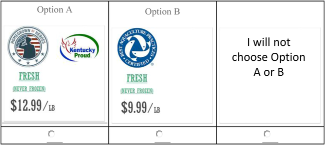
Figure 1. Example of a sample choice card in the choice experiment.
To gauge whether respondents read and understood the information presented (for each of the three attributes), a participant was presented a statement, and asked to indicate whether the statement was true or false based on the information presented earlier. Participants could retract and revisit the web page providing information on the attributes. For each attribute, shown randomly, either a true or a false statement would appear. In other words, the authors prepared both a true and a false statement for each attribute; however, each participant was randomly presented one for each attribute. Appendix B displays the statements. These statements were created after intensive discussion with experts and general consumers. Whether participants answered each of these questions correctly was used to model their choices. A total of 63% and 65% of the respondents answered all three questions correctly in Kentucky and South Carolina, respectively.
Participants were then instructed to proceed with a choice card and select one of the three options provided. Respondents were informed that all other product characteristics were identical for each situation (except the attributes explicitly presented). Finally, participants were reminded not to compare across situations as if they were shopping in a grocery store. Appendix C presents an abbreviated version of the survey instrument.
4. Data
Data were collected from a total of 1,011 respondents (505 from Kentucky and 506 from South Carolina). Qualtrics, a large online panel of general consumers, was contracted to distribute the survey. Specific information regarding the sampling process, such as response rate, is proprietary. Nevertheless, Table 2 provides selected sociodemographic statistics for the two states from the 2012 American Community Survey, as well as the sample demographics. Female respondents made up the majority of survey participants (about 69%), but this makes intuitive sense when considering the female role in shopping behavior. For example, females resulted in 60% of the Fonner and Sylvia (Reference Fonner and Sylvia2014) sample when analyzing WTP for seafood attributes. In order to proceed with the survey, participants had to respond “yes” to whether they classified themselves as the primary grocery shopper. Most survey respondents were between the ages of 35 and 54 (43%). When asked about education, “some college, technical school, or associate’s degree” was the majority response (37%), and most respondents earned $50,000 to $74,000 (17%) annually.
Table 2. Sample and population sociodemographic statistics

a State population is based on 25 years and over.
b In 2014 inflation-adjusted dollars.
Note: State population statistics are based on the 2012 American Community Survey 1-year estimates.
5. Model
Lancaster’s (Reference Lancaster1966) formative study creates the framework to evaluate consumers’ utility for products with an array of attributes. By recognizing that a collection of traits is significant, Lancaster (Reference Lancaster1966) proposed the theory of demand for products having one or more attributes.
When considering a number of n-choice situations and evaluating consumer i’s selection of a product, McFadden’s (Reference McFadden and Zarembka1974) random utility theory can be applied. Consumer i’s indirect utility (U ijn ) from selecting the jth product in a group of J products in the nth choice condition (n = 1, 2, 3, …) is described as a linear function of product attributes (X ijn ) by the following equation:
 $${U_{ijn}} = {\boldsymbol X_{ijn}}{\boldsymbol\beta} + {\varepsilon _{ijn}},$$
where β symbolizes a vector of indefinite marginal utilities from product attributes X ijn of the alternate j in choice situation n, and ε ijn denotes the random error term of the computed utilities. Assuming that consumers act rationally, utility is maximized through selecting alternatives j in the nth choice framework (McFadden, Reference McFadden and Zarembka1974).
Owing to the extensive application of the conditional logit (CL) choice model for inference in discrete choice experiments, this econometric technique is applied as a baseline model in this research as well. By accepting that the independent and identical distribution (iid) of the error term (ε ijn ) and independence of irrelevant alternatives (IIA) assumptions hold, the probability of the jth option being selected can be modeled as follows:
 $$P({Y_{in}} = j) = {{{\rm{exp}}(\boldsymbol{X_{ijn}}\boldsymbol\beta )} \over {\sum _{j = 1}^J{\rm{exp}}(\boldsymbol{X_{ijn}}\boldsymbol\beta )\;}}\;\;\;\;{\rm{For}}\;j = 1,2,\;...\;J,$$
where Y in is an indicator variable representing the selection by consumer i in the nth choice situation. Considering a closed-form probability function, the CL method can be assessed using maximum likelihood estimation (McFadden, Reference McFadden and Zarembka1974). Though straightforward to estimate, the IIA assumption is restrictive. Train (Reference Train1998) developed an alternative to CL known as the mixed logit model. The mixed logit offers greater flexibility by relaxing the IIA assumption and incorporating preference heterogeneity, as well as accounting for correlations between multiple choice observations made by each respondent (Bliemer and Rose, Reference Bliemer and Rose2010). This is also referred to as accounting for correlation in unobserved utility over repeated choices made by each respondent, or that the parameter estimates of the marginal utilities vary across respondents. The choice probability identified by the mixed logit is modeled as
 $$P({Y_{in}} = j) = \int {{{{\rm{exp}}(\boldsymbol{X_{ijn}} \boldsymbol\beta )} \over {\sum _{(j = 1)}^J{\rm{exp}}(\boldsymbol{X_{ijn}}\boldsymbol\beta )}}} f(\boldsymbol\beta )d\boldsymbol\beta ,$$
where the coefficients in vector β are defined as random variables following density function f as
 $${\beta _i} \sim f\left( {{\beta _{0,}}\;\boldsymbol G} \right),$$
with β 0 as the means of β i and G as the variance matrix. With the probability evaluated over a range of possible values of β i and the absence of a closed-form solution, the approach of approximating the likelihood function with simulated maximum likelihood is applied to the model (Train, Reference Train2009).
Following the estimation of β in either the conditional or mixed logit model, marginal WTP measures for an attribute k is approximated as the coefficient estimate for the attribute divided by the negative marginal utility of price (Louviere, Hensher, and Swait, Reference Louviere, Hensher and Swait2000):
 $$WT{P_k} = - {{{\beta _k} + {\boldsymbol\beta _{\boldsymbol kD}} \times \boldsymbol D} \over {{\rm{\beta _{\rm price}}}}}$$
where D are covariates entered as interactions with the attributes in the logit model to further decompose the main effect of attribute k, and βkd are the coefficients associated with the interaction effects. Thus, WTP measures the change in price associated with a unit increase in the respective attribute and approximates the monetary values of product attributes.
6. Results
The null hypothesis that the estimates are equivalent between the two samples was rejected by a joint F-test. As a result, data of the two states were estimated separately. Parameter estimation results for the mixed logit models are presented in Tables 3 and 4 for the Kentucky and South Carolina samples, respectively. A simulated maximum likelihood estimator with 1,000 Halton draws was utilized for the estimation.
Table 3. Mixed logit model estimation result—Kentucky sample

Notes: Asterisks (*, **, and ***) indicate significance at the 10%, 5%, and 1% level, respectively. BAP, Best Aquaculture Practices; CSF, Community-Supported Fishery; HBH, Homegrown by Heroes.
Table 4. Mixed logit model estimation result—South Carolina sample

Notes: Asterisks (*, **, and ***) indicate significance at the 10%, 5%, and 1% level, respectively. BAP, Best Aquaculture Practices; CSF, Community-Supported Fishery; HBH, Homegrown by Heroes.
For each state, the main effect utility parameter included coefficients for a series of dummy variables: Fresh (baseline is “previously frozen”), Local (baseline is “unlabeled”), BAP (baseline is “unlabeled”), CSF (baseline is “unlabeled”), HBH (baseline is “unlabeled”), and Price (four levels). The model formulations also included interaction effects. Specifically, the abovementioned main effects were interacted with the following variables: Age, Education level (Edu), Income (annual pretax income),Footnote 2 Child (dummy variable indicating minors present in household), Employed (dummy variable indicating at least partially employed), Coast (dummy variable indicating growing up within 50 miles of a coast), and Identified (dummy variable indicating correctly answering true/false question). Other possible variables, such as whether a household had any direct family members with military service, were tested; however, these were not statistically significant in any formulation and thus were not included in the final model. Potential multicollinearity was checked by calculating the coefficient of correlation matrix of all variables used in the models; about 0.6% of the correlation coefficients were greater than 0.5 in absolute values. Readers are reminded of the possible minor multicollinearity. For the purpose of comparison, mixed logit model results incorporating only the main effects are reported in Appendix D. The result is highly consistent with the models including interactions.
Finally, a normal distribution was assumed for all main effect coefficients except the price. This is to avoid unrealistic WTP distributions associated with the ratio between two distributions (Carson and Czajkowski, Reference Carson and Czajkowski2019). The standard deviation of all random coefficients is presented alongside the corresponding main effect coefficients.
The variable “No choice” is a dummy variable indicating the third alternative in each choice set. It represents the opposite of the utility associated with the sum of the omitted levels for each attribute (Adamowicz et al., Reference Adamowicz, Swait, Boxall, Louviere and Williams1997), and as a result, its value depends on how each attribute is defined and entered into the model. In other words, it depends on the level omitted for each dummy variable. We focus on interpreting the coefficients associated with the attributes. Because the models presented in Tables 3 and 4 include interaction terms to further explain the main effects of the attributes, the coefficient estimates of the main effects cannot be explained alone. All interaction effects must be jointly considered, which is conducted when the WTP measures are calculated. Nevertheless, the standard deviation estimates of the main effects and the direction of the interaction effects can be explained. For both states, the standard deviation estimates of random coefficients for Fresh (Never Frozen), Local, and HBH are highly significant, suggesting a large degree of heterogeneity in consumer taste. Standard deviation estimates of the random coefficients BAP and CSF are not statistically significant.
For the Kentucky sample (Table 3), participant age has a negative impact on utility associated with the CSF attribute. This suggests that, holding all other factors constant, older consumers are less likely to purchase CSF-labeled product. Education appears to affect consumer perception on several attributes. For the BAP and HBH labels, higher education leads to greater utility while also making consumers more price sensitive. Participant income strengthens the preference of the HBH attribute. Having at least one child living within the household makes consumers more in favor of the HBH attribute and not as sensitive to price. Participants with at least a part-time job are less sensitive to product price. Consumers growing up within 50 miles of the coast are less likely to purchase shrimp with “Kentucky Proud” (i.e., local) label and are less price sensitive. Answering the true or false question correctly is strongly and positively related to consumer utility associated with the HBH attribute. This suggests that consumers who understand the HBH label correctly have a higher value associated with the attribute. For all other attributes, there are no significant effects of answering the true or false questions correctly.
For the South Carolina sample (Table 4), participant age has a positive interaction effect with the HBH attribute, indicating older consumers are more likely to value the HBH attribute. Participants with higher education attainment place greater emphasis on Local as well as BAP. Although income does not seem to have a significant interaction effect with any product attribute, consumers with at least one child in the household are willing to pay more for products labeled Local and BAP. Compared with no employment, partial or full employment is associated with less WTP for BAP and HBH attributes, as well as less price sensitivity. Growing up within 50 miles of a coast has no effect on any attributes, only leading to less price sensitivity. Similar to the case for Kentucky, the HBH label was the sole significant attribute for significant and positive effects for participants answering the true or false question correctly.
Consumer preference is best reflected by WTP after considering all main and interaction effects jointly. Table 5 presents the WTP estimates following equation (4). All WTP standard deviations are estimated using the simulation approach described by Krinsky and Robb (Reference Krinsky and Robb1986) with 5,000 iterations. These standard deviation estimates reflect the standard errors in the mixed logit models. The focus and discussion pertained to the mean effects. At the top of the table, a list of sample means (median for discrete variables) is given for each variable used as a covariate interacting with the main effect attributes. When calculating WTP, all covariates are held at the sample mean/median unless the interaction is at least significant at the 10% level in Table 3 or 4. In this case, different values of the covariate variables are considered to show the WTP’s impact.
Table 5. Willingness to pay (WTP) of different consumer profiles

a Standard errors are calculated through simulation with 5,000 iterations.
b WTP for each attribute measured at sample mean/median is displayed after “Sample mean” under each attribute. If some interactions are significant, WTPs are calculated under different values of the interactions. For instance, the only significant interaction for Local in the Kentucky sample is with variable Coast. As a result, although sample mean WTP reflects all variables held at sample mean/median, which suggests that Coast = 0, because this interaction is significant, we also calculate the WTP when all other variables are held at sample mean/median, except that Coast = 1 instead. The same applies to other attributes.
Note: BAP, Best Aquaculture Practices; CSF, Community-Supported Fishery; HBH, Homegrown by Heroes.
First, the WTP for each attribute is calculated at the sample mean/median for each state. Comparing the two states, Kentucky consumers show more preference and WTP for Local, BAP, and HBH-labeled products. For Kentucky, the interacted terms for the attribute “Fresh (Never Frozen)” are all insignificant. As a result, the WTP of Kentucky consumers on shrimp that are fresh is measured at the sample mean, resulting in $6.33/lb. compared with frozen while holding all other factors constant between these two product types. For the Kentucky Proud label, covariate variable “Coast” is significant. Thus, two consumer types are considered: participant A grew up within 50 miles of a coast, whereas participant B did not, as both have all other characteristics at the sample average. Participant B represents a sample average consumer as most of those sampled (i.e., did not grow up near a coast). Growing up near a coast has much less WTP for Local shrimp than the contrary. This is expected because Kentucky is an inland state; those who grew up near a coast are likely not originally from Kentucky. Residents with a profound coastal background are more likely to prefer products from that home state.
Following a similar logic, three levels of education are considered for the attribute BAP, while holding all other covariates at the sample average. WTP for the BAP attribute relative to products without the BAP attribute increases along with higher education. Among the lowest educated consumers, WTP is negative and suggests that consumers are not willing to pay anything for this attribute. On the other hand, consumers with the highest level of education are willing to pay as high as $3.27/lb. for the BAP attribute; sample average education consumers are willing to pay $2.45/lb.
Overall, CSF is not an attribute consumers prefer. However, consumer age significantly affects WTP for the CSF attribute. Despite variation in age, the WTP for CSF is largely negative compared with products not from a CSF. This reluctance in supporting CSF may be a reflection of consumer concern about the quality of products coming from a CSF because freshness is of high importance, as products not allocated to CSF shares may be perceived less fresh.
Sharply in contrast with CSF, the HBH attribute receives strong WTP across all consumer profiles. WTP for HBH at the sample average is $2.82/lb. Highly educated or having at least one child living in the household are more supportive to the label; the WTP for those with at least one child at home is as high as $6.99/lb. Not understanding the HBH label (i.e., answered the true or false question incorrectly) leads to a great reduction in WTP measured at only $0.45/lb. more compared with a non-HBH product, holding all other attributes common across products.
Turning to South Carolina, education is a significant explanatory factor in consumer WTP for fresh shrimp, although the WTP does not change drastically across education. For Local, higher education favors this attribute along with having at least one child in the household. Consumer WTP for the BAP attribute is generally not high. Education (1), whether the household has at least one child at home (2), and employment status (3) are all significant determinants, and the WTP typically ranges from about $2 to $3/lb. for different consumer profiles. For the CSF attribute, like Kentucky consumers, the WTP is nearly nonexistent.
South Carolina consumers are also fond of the HBH attribute. In general, older consumers are more supportive. For consumers 65 and older, WTP is as high as $3.82/lb. compared with non-HBH shrimp. Employment status is statistically significant, but the corresponding WTP for HBH shrimp is not economically different regardless of whether the participant is employed or not. A large gap in WTP exists between whether a participant could correctly identify the truthfulness of a statement about the attribute. Greater understanding of the label is attributed to paying $2.68/lb. more for HBH shrimp compared with $0.43/lb. for those who do not understand the HBH product (signified by answering the true or false question incorrectly).
7. Conclusion and implications
By considering inland Kentucky and coastal South Carolina, we investigated consumer preferences for shrimp with multiple attributes. With a strong focus toward developing marketing strategies, the attributes examined were deemed possible candidates for producers and policy makers to adopt. By including unfamiliar, emerging, and hypothetical labels, we also contribute to the literature by establishing a foreground for further research.
Survey results had implications for both existing and developing attributes for the shrimp market. Consistent with previous studies, product form (i.e., “Fresh [Never Frozen]” or “Previously Frozen”) produced the highest premium, with both states garnering this result. Criteria referring to product form may infer how customers evaluate quality such as taste, sight, and smell of the product, with results indicating a fresh form consisting of a higher quality versus a previously frozen product. Results showing some South Carolina residents willing to pay higher premiums could suggest living in a coastal state, with closer proximity and access to fresh products, may generate greater preference for nonfrozen products.
Concerning the popularity of the local food movement and support for producers operating within participants’ state of residence, a “local” label allowed for analysis on preference for regional seafood. Although the literature is extensive, this study provided additional context of seafood labeling under which the “local” term was compared with other shrimp attributes. In both states, the “local” state labels generated the second highest premium behind product form, implying that support for shrimp sourced within the state is highly valued. Producers of aquaculture systems could use these results to justify labeling schemes indicating state origin, which ultimately may be more important than attributes such as environmental certification.
With the BAP label signifying environmental standards and sustainable practices, significant premiums resulted in both states, though not as strong as the product form and local attributes. Considering the relative magnitude of results, consumers may not fully understand nor value environmental stewardship as strongly in the case of aquaculture products. A possible explanation for this finding is that within aquaculture production systems, issues such as bycatch and stock (or supply) of certain seafood species is not as relevant as in ocean capture, so the value of certification may be limited. The only negative though insignificant product feature was the “Product of CSF” attribute. This could be the result of consumers’ concerns regarding the quality of farm-raised seafood in a CSF context.
Consumer perception of veteran-sourced products has not been studied within the food literature. Despite the recent emergence of Homegrown by Heroes (as of 2013) and existence in today’s food markets, the label was shown to be significant and produce a premium that was marginally less than “local” labels. Similar results between both states add to the importance of results. Policy makers may be encouraged to expand promotion and work with the Farmer Veteran Coalition to further develop and promote marketing programs for veterans in food production. Last, it is important to highlight that the WTP estimates are addable to each other. Thus, seafood producers can realize substantial premiums if their products include all the positive attributes.
For this study, we would like to mention limitations to better understand how future research can progress. First, the study includes two U.S. states located in the southeastern region; thus, it is hard to justify national implications. Although limiting our study to two states enables us to provide a more focused discussion on similarities and differences, future projects may survey a broader audience with greater sampling. Results can then be assessed from a national perspective, and more robust conclusions can be drawn on.
National scale is not the only market targeted when considering the global nature of the seafood market. A study of multiple consumers across various countries can support the understanding of international trade, as disputes considering the inflow of imported seafood products (e.g., shrimp) continue to affect domestic markets. An additional concern is the impact of wild-caught fisheries and environmental issues from a global scale, so consumer research in multiple countries could help understand preference in these areas.
Second, this study focuses only on the demand side of the market. Although it has been shown there is positive consumer support for many of the attributes considered, one must assess the feasibility of implementing these various labels by producers. With both mislabeling and transparency being prominent issues affecting the seafood supply chain, the supply side (or processing and distribution) must be considered, especially in strategizing marketing programs successfully. Future research may include developing producer surveys to analyze whether participation in certain programs would occur and if labels justify the economic investment to follow certain standards.
Third, the current analysis provides a snapshot of seafood consumption focusing on farm-raised shrimp. Certain participants who do not prefer shrimp or assess seafood attributes for other seafood species from a different perspective may affect conclusions made about certain labels. Studying other popular forms of seafood (e.g., salmon, tuna, etc.) could make conclusions more robust. A broader understanding of the overall consumption and, more important, long-term consumption trends is an interesting area for future research. Though many attributes included are emerging within the marketplace, one must also assess the sustainability of demand for future implementation.
Supplementary material
To view supplementary material for this article, please visit https://doi.org/10.1017/aae.2019.19
Acknowledgments
The authors would like to thank the anonymous reviewers for the beneficial feedback.
Financial support
This study is partially funded by Clemson University. Funding from the University of Kentucky and The Ohio State University is also appreciated.
Conflicts of interest
None.


 Open access